Effect of Turbulence Inhibitors on Molten Steel Flow in 66-Ton T-Type Tundish with Large Impact Area


Abstract
:1. Introduction
2. Description of Numerical Simulation and Hydraulics Experiment Process
2.1. Numerical Simulation
2.1.1. Basic Assumptions
- (1)
- The fluid flow in the tundish is treated as steady state flow, and the fluid is considered as Newtonian and incompressible.
- (2)
- The effect of temperature on the density of the steel, slag and tracer are ignored. The density of the steel, slag and tracer are constant.
- (3)
- In the tundish, the steel, slag and tracer are treated as homogeneous medium.
- (4)
- The liquid-liquid interface is set to non-slip wall boundary, meaning that the velocity at the wall is 0, k = 0 and ε = 0.
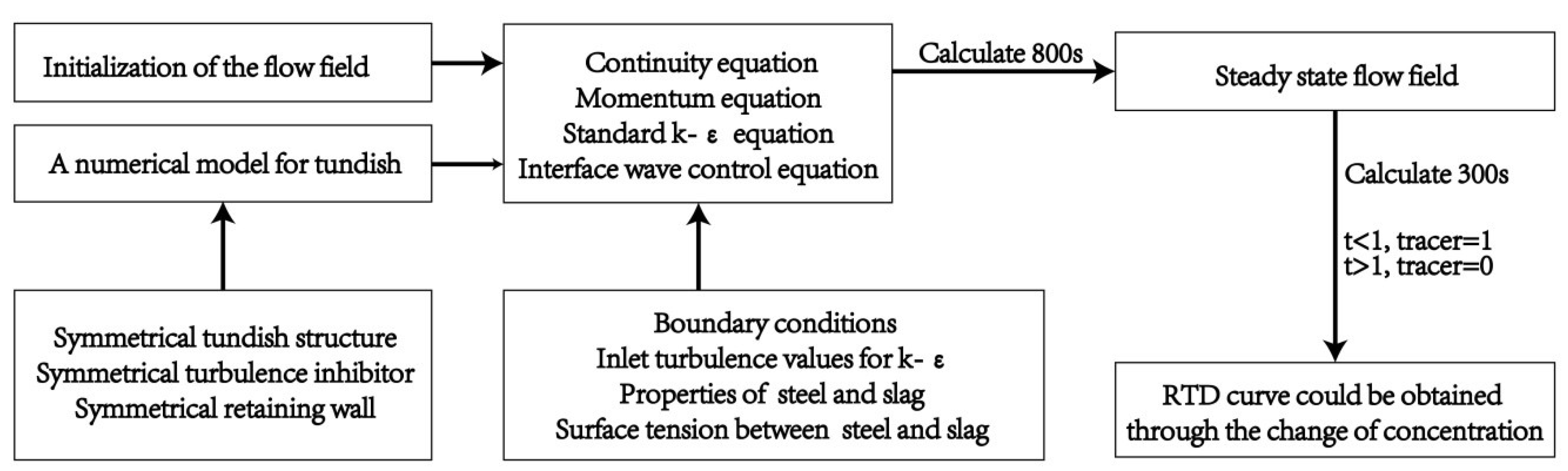
2.1.2. Mathematical Models
- (1)
- Continuity equation could be expressed as follows:
- (2)
- Momentum equation (Navier-Stokes equation) could be expressed as follows:
- (3)
- (4)
- Interface wave control equation
2.1.3. Boundary Conditions
- (1)
- The velocity inlet boundary condition was applied for the computational inlet. The velocity of molten steel was calculated according to the volume flow of the inlet and the cross-section area of the ladle shroud. The turbulent kinetic energy and the turbulent energy dissipation rate of the inlet can be obtained by Equations. and respectively. Where, is the inlet velocity, m·s−1, is the inner diameter of ladle shroud, m.
- (2)
- The outflow boundary condition was applied for the computational outlet.
- (3)
- The top of the tundish was set as a free surface with shear force of zero.
- (4)
- No slip boundary condition at the wall and standard wall function near the wall has been applied.
2.1.4. Numerical Method
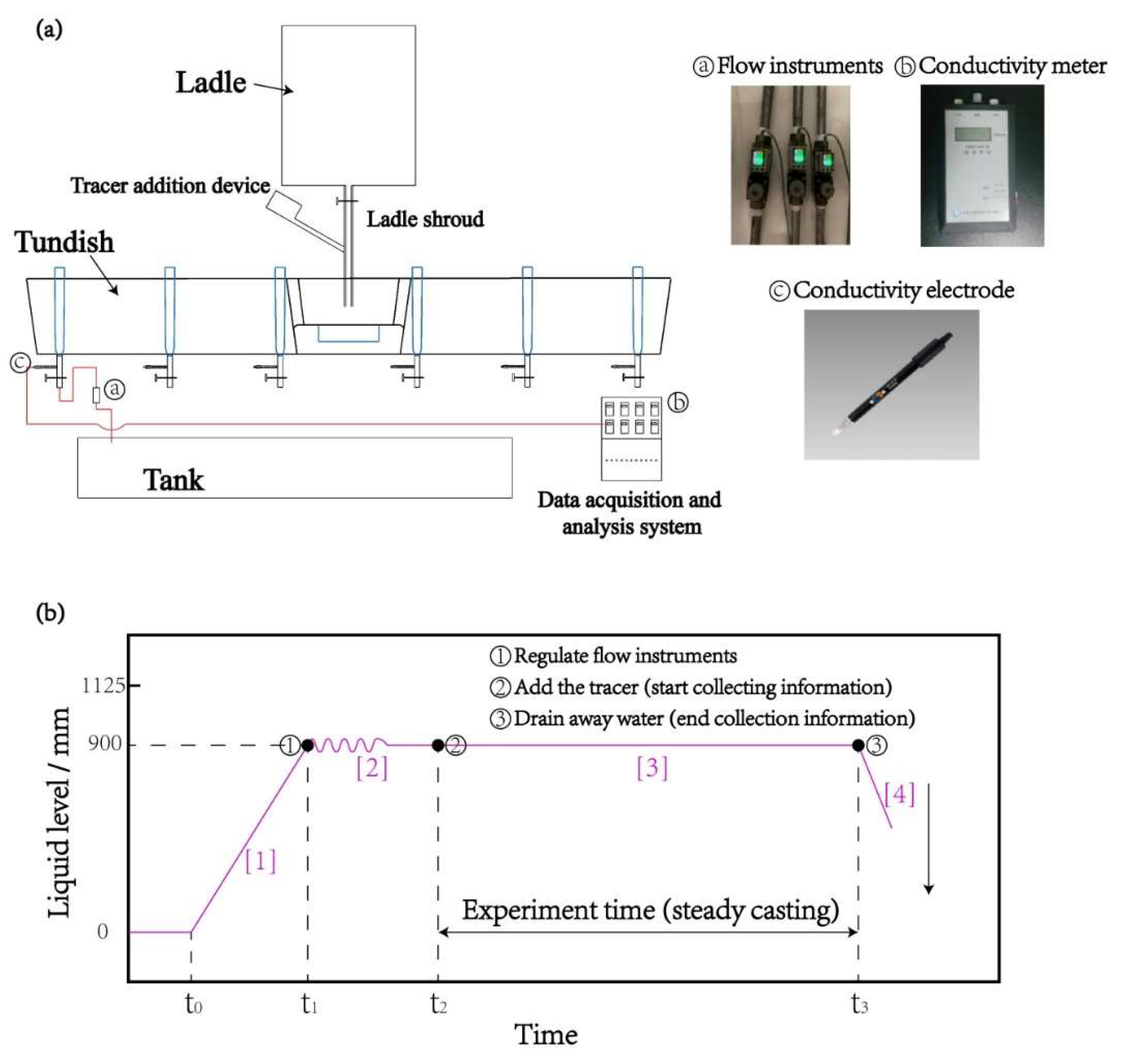
2.2. Hydraulics Experiment
3. Results and Discussion
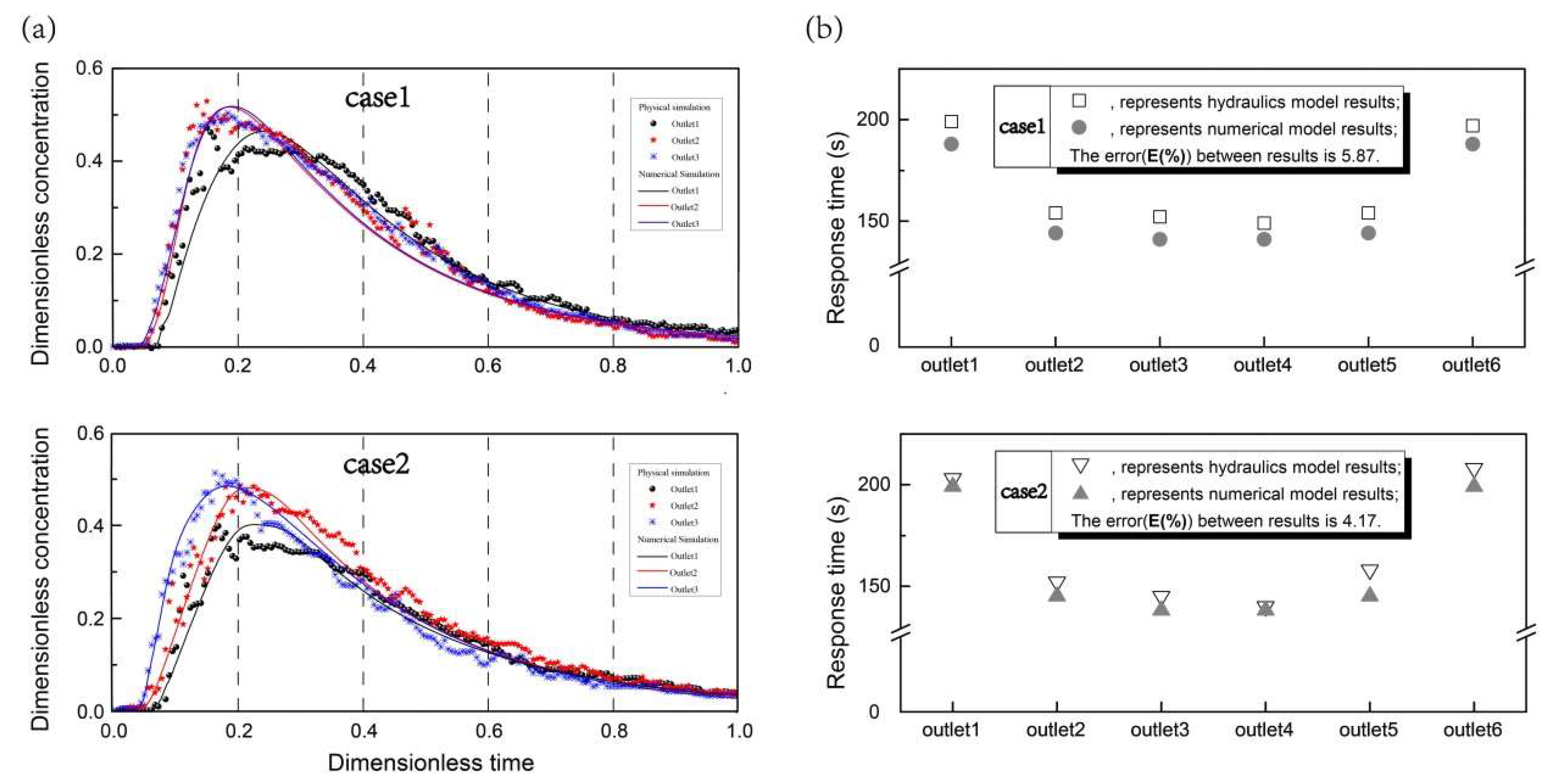
3.1. Model Validations and Analysis of Response Time
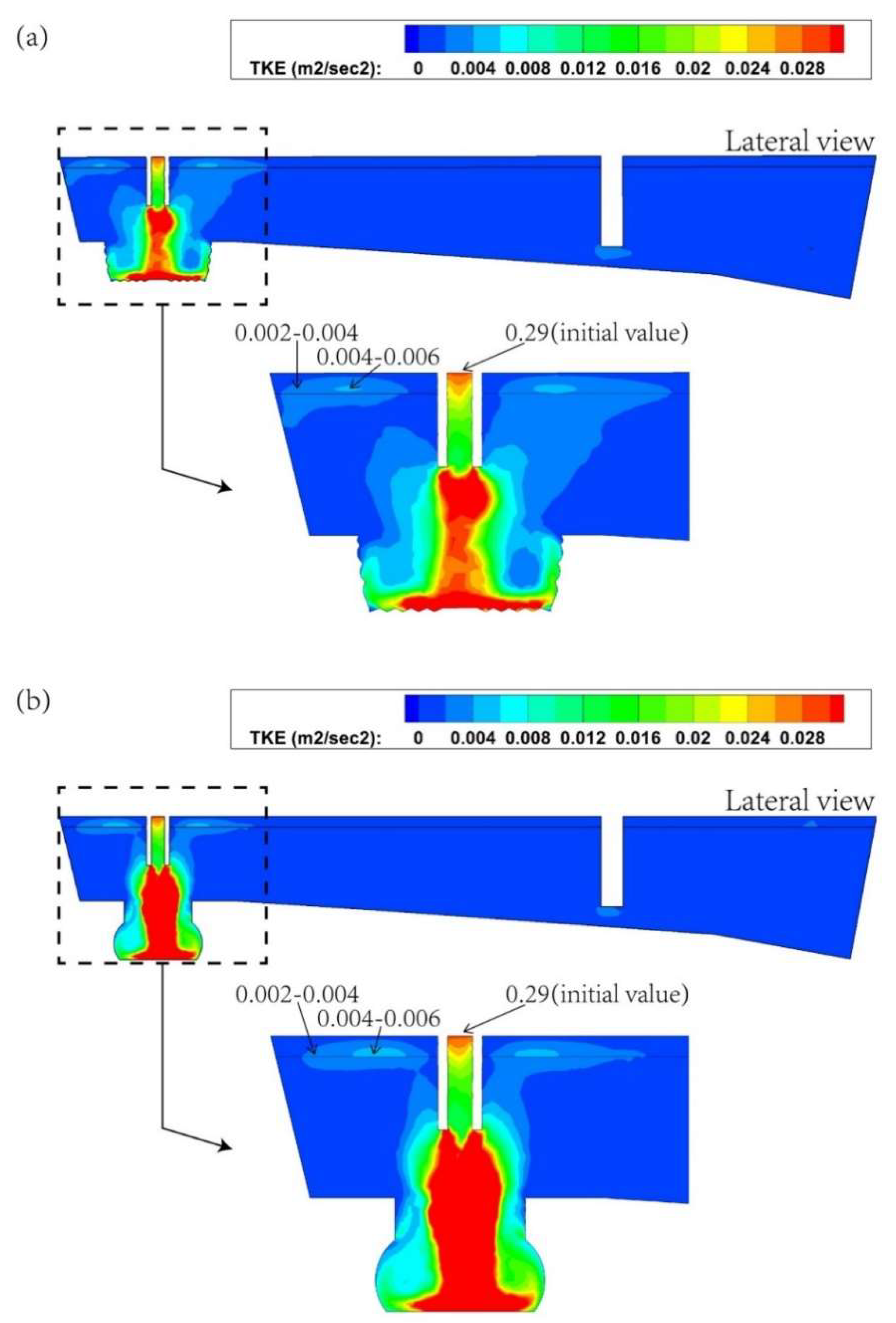
3.2. Jet Flow and Turbulent Kinetic Energy in Two Cases
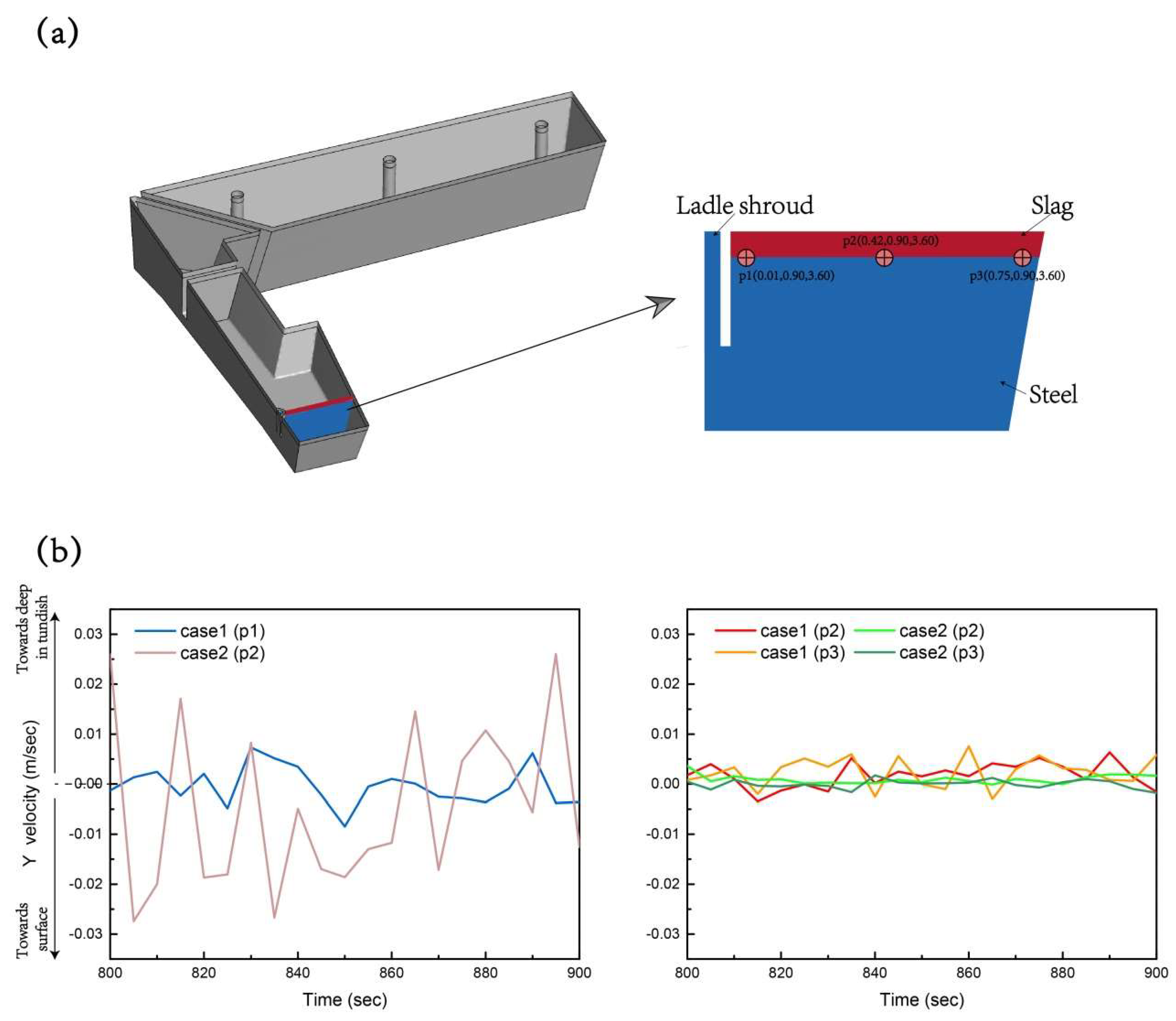
3.3. The Fluctuation of Steel-Slag Interface in Two Cases
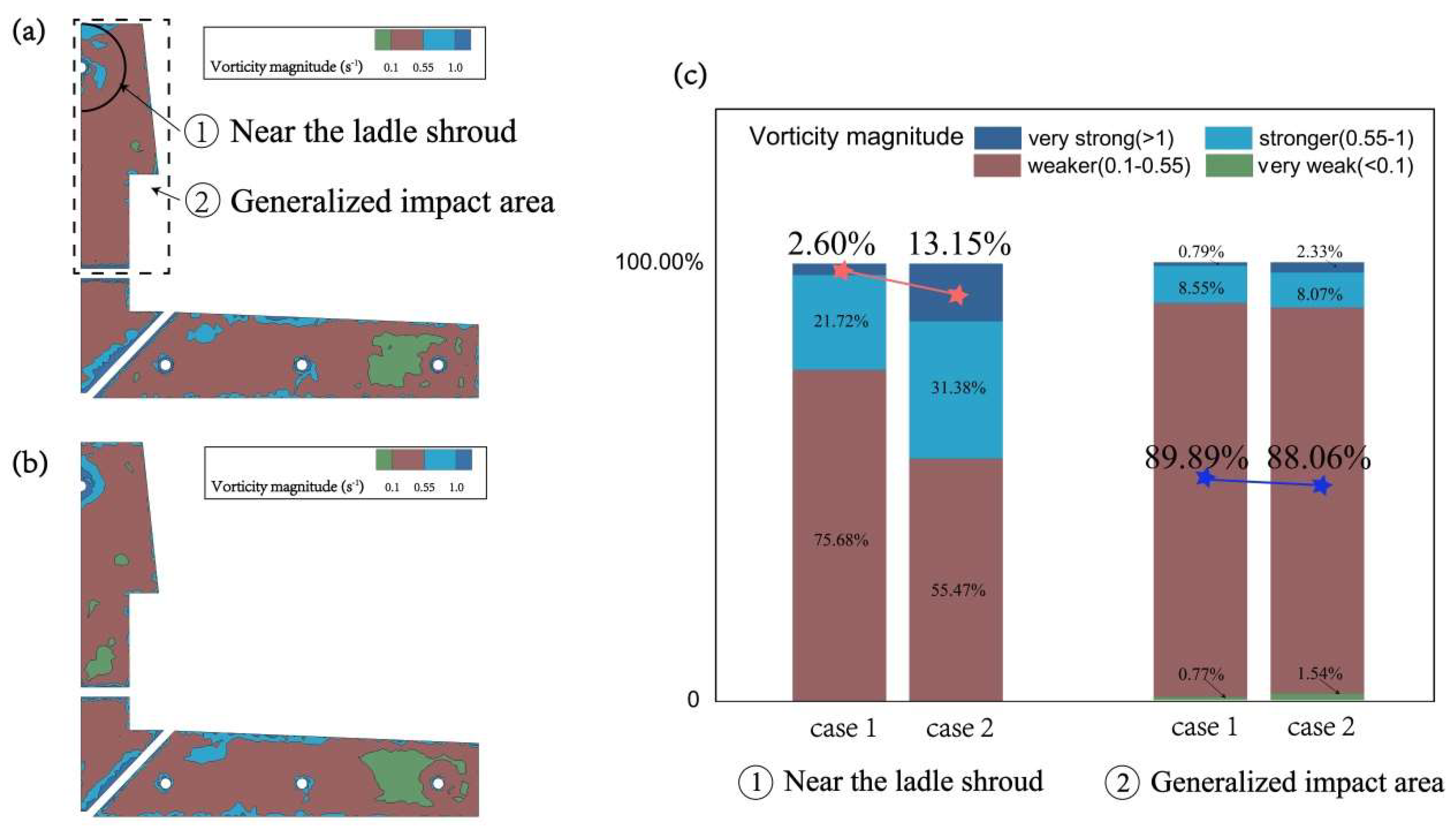
3.3.1. Analysis of Vorticity Magnitude
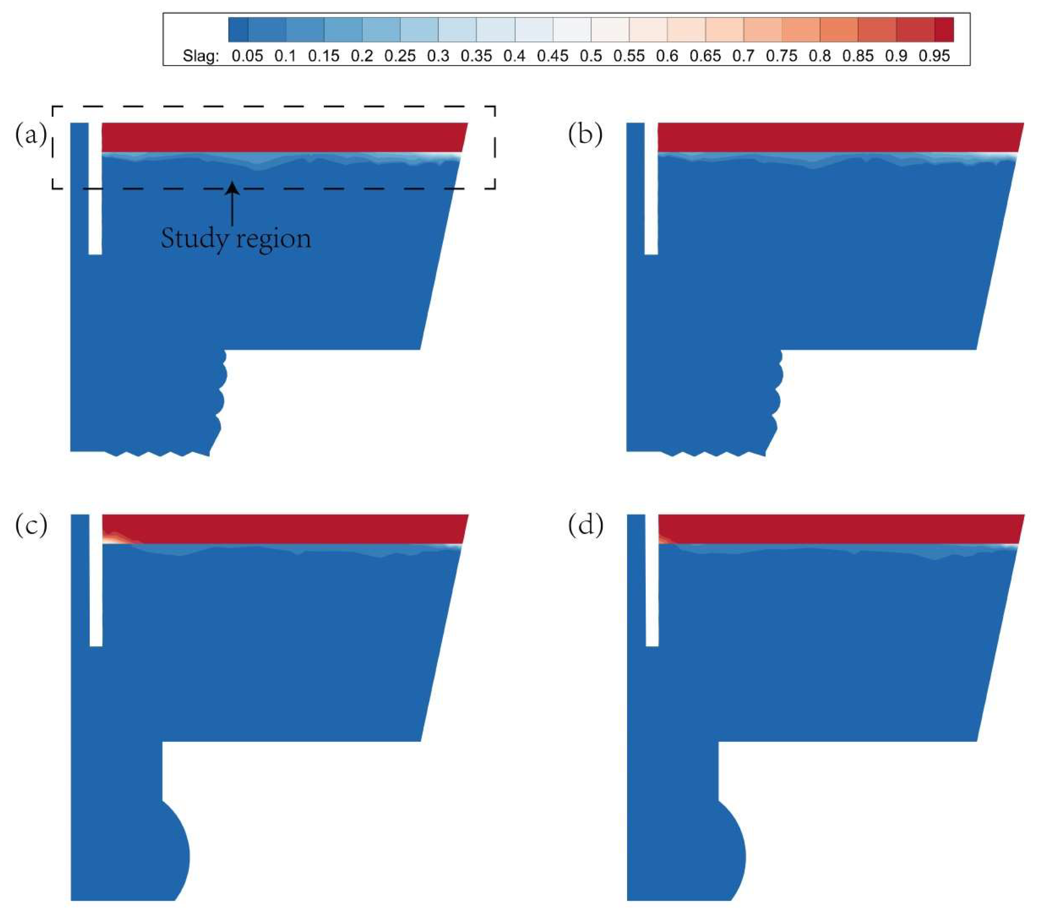
3.3.2. Analysis of Transient Interface Change
4. Conclusions
- (1)
- A human-defined virtual phase (tracer) with the same properties as steel is introduced to calculate the RTD curve of each strand through the VOF model, and the error was less than 6% compared with the numerical simulation result, which could prove the reliability of the numerical simulation results.
- (2)
- Jet flow into the tundish generated very different flow patterns. Case 1 produced a double-roll flow pattern and case 2 produced a four-roll flow pattern in the impact area. The turbulence inhibitor can fully consume the velocity and turbulence of molten steel both in case 1 and case 2. However, case 2 had two vortices under the turbulence inhibitor, which could cause some molten steel to directly impact the steel-slag interface along the tangential direction of the vortices and slag entrainment may occur during the process.
- (3)
- The ratio of vorticity magnitude between 0.10–0.55 s−1 (in this range, steel-slag flow state is the best) in the generalized impact area in case 1 and in case 2 were close. However, the ratio of vorticity magnitude above 1.00 s−1 near the ladle shroud was 2.60% in case 1, the ratio of vorticity magnitude above 1.00 s−1 near the ladle shroud was 13.15% in case 2 and this ratio in case 2 is five times that in case 1, which indicates case 2 increased the possibility of slag entrainment via the upward flow mechanism and shear layer instability.
- (4)
- Near the ladle shroud, the maximum surface velocity of case 2 was almost three times that of case 1, and surface velocity fluctuations were much more severe. The thickness of the slag layer was 60 mm, and the interface fluctuation towards surface in case 2 was close to 20 mm, which can cause surface instability and slag entrapment. Case 1 involved very small volume-fraction contours in this region.
- (5)
- The turbulence inhibitor with internal ripples (case 1) had more obvious optimization effect, which can provide a theoretical basis for selecting suitable turbulence inhibitor for the 66-ton T-type tundish with large impact area.
Author Contributions
Funding
Conflicts of Interest
References
- Ding, N.; Bao, Y.P.; Sun, Q.S. Optimization of flow control devices in a single-strand slab continuous casting tundish. Int. J. Miner. Metall. Mater. 2011, 18, 292–296. [Google Scholar] [CrossRef]
- Bensouici, M.; Bellaouar, A.; Talbi, K. Numerical investigation of the fluid flow in continuous casting tundish using analysis of RTD curves. J. Iron Steel Res. Int. 2009, 16, 22–29. [Google Scholar] [CrossRef]
- Bai, H.; Thomas, B.G. Turbulent flow of liquid steel and argon bubbles in slide-gate tundish nozzles: Part I. model development and validation. Metall. Mater. Trans. B 2001, 32, 253–267. [Google Scholar]
- Bai, H.; Thomas, B.G. Turbulent flow of liquid steel and argon bubbles in slide-gate tundish nozzles: Part II. effect of operation conditions and nozzle design. Metall. Mater. Trans. B 2001, 32, 269–284. [Google Scholar] [CrossRef]
- Xing, F.; Zheng, S.G.; Zhu, M.Y. Motion and removal of inclusions in new induction heating tundish. Steel Res. Int. 2018, 89, 1700542. [Google Scholar] [CrossRef]
- Yang, B.; Lei, H.; Jiang, J.M. Electromagnetic conditions in a tundish with channel type induction heating. Steel Res. Int. 2018, 89, 1800145. [Google Scholar] [CrossRef]
- Yue, Q.; Zhang, C.B.; Pei, X.H. Magneto hydrodynamic flows and heat transfer in a twin-channel induction heating tundish. Ironmak. Steelmak. 2017, 44, 227–236. [Google Scholar] [CrossRef]
- Palafox-Ramos, J.; Barreto, J.D.; Lopez-Ramírez, S. Melt flow optimisation using turbulence inhibitors in large volume tundishes. Ironmak. Steelmak. 2001, 28, 101–109. [Google Scholar] [CrossRef]
- Merder, T.; Pieprzyca, J. Optimization of two-strand industrial tundish work with use of turbulence inhibitors: Physical and numerical modeling. Steel Res. Int. 2012, 83, 1029–1038. [Google Scholar] [CrossRef]
- Morales, R.D.; Lopez-Ramírez, S.; Palafox-Ramos, J. Mathematical simulation of effects of flow control devices and buoyancy forces on molten steel flow and evolution of output temperatures in tundish. Ironmak. Steelmak. 2001, 28, 33–43. [Google Scholar] [CrossRef]
- Liu, S.X.; Yang, X.M.; Du, L. Hydrodynamic and mathematical simulations of flow field and temperature profile in an asymmetrical T-type single-strand continuous casting tundish. ISIJ Int. 2008, 48, 1712–1721. [Google Scholar] [CrossRef] [Green Version]
- Merder, T.; Pieprzyca, J.; Saternus, M. Analysis of residence time distribution (RTD) curves for T-type tundish equipped in flow control devices: Physical modeling. Metalurgija 2014, 53, 155–158. [Google Scholar]
- Warzecha, M.; Merder, T.; Warzecha, P. CFD modelling of non-metallic inclusions removal process in the T-type tundish. J. Achievements. Mater. Manuf. Eng. 2012, 55, 590–595. [Google Scholar]
- Jin, Y.; Ye, C.; Luo, X. The model analysis of inclusion moving in the swirl flow zone sourcing from the inner-swirl-type turbulence controller in tundish. High Temp. Mater. Processes 2017, 36, 541–550. [Google Scholar] [CrossRef]
- Yang, S.F.; Li, J.S.; Jiang, J. Fluid flow in large-capacity horizontal continuous casting tundishes. Int. J. Miner. Metall. Mater. 2010, 17, 262–266. [Google Scholar] [CrossRef]
- Merder, T.; Pieprzyca, J. Numerical modeling of the influence subflux controller of turbulence on steel flow in the tundish. Metalurgija 2011, 50, 223–226. [Google Scholar]
- Chen, D.F.; Xie, X.; Long, M.J. Hydraulics and mathematics simulation on the weir and gas curtain in tundish of ultrathick slab continuous casting. Metall. Mater. Trans. B 2011, 45, 392–398. [Google Scholar] [CrossRef]
- Zhang, J.S.; Liu, Q.; Yang, S.F. Advances in ladle shroud as a functional device in tundish metallurgy: A review. ISIJ Int. 2019, 59, 1167–1177. [Google Scholar] [CrossRef] [Green Version]
- Yang, B.; Lei, H.; Zhao, Y. Quasi-symmetric transfer behavior in an asymmetric two-strand tundish with different turbulence inhibitor. Metals 2019, 9, 855. [Google Scholar] [CrossRef] [Green Version]
- Mishra, R.; Mazumdar, D. Numerical analysis of turbulence inhibitor toward inclusion separation efficiency in tundish. Trans. Indian Inst. Met. 2019, 72, 889–898. [Google Scholar] [CrossRef]
- Merder, T. The influence of the shape of turbulence inhibitors on the hydrodynamic conditions occuring in a tundish. Arch. Metall. Mater. 2013, 58, 1111–1117. [Google Scholar] [CrossRef]
- Warzecha, M.; Merder, T.; Pfeifer, H. Investigation of flow characteristics in a six-strandcc tundish combining plant measurements, physical and mathematical modeling. Steel Res. Int. 2010, 81, 987–993. [Google Scholar] [CrossRef]
- Solorio-Díaz, G.; Morales, R.D.; Palafax-Ramos, J. Analysis of fluid flow turbulence in tundishes fed by a swirling ladle shroud. ISIJ Int. 2004, 44, 1024–1032. [Google Scholar] [CrossRef]
- Qin, X.F.; Cheng, C.G. A simulation study on the flow behavior of liquid steel in tundish with annular argon blowing in the upper nozzle. Metals 2019, 9, 225. [Google Scholar] [CrossRef] [Green Version]
- Zhang, H.; Luo, R. Numerical simulation of transient multiphase flow in a five-strand bloom tundish during ladle change. Metals 2019, 8, 146. [Google Scholar] [CrossRef] [Green Version]
- Morales, R.D.; Guarneros, J. Fluid flow control in a billet tundish during steel filling operations. Metals 2019, 9, 394. [Google Scholar] [CrossRef] [Green Version]
- Cwudziński, A. Numerical and physical modeling of liquid steel active flow in tundish with subflux turbulence controller and dam. Steel Res. Int. 2014, 85, 902–917. [Google Scholar] [CrossRef]
- Cwudziński, A. Numerical, physical, and industrial experiments of liquid steel mixture in one strand slab tundish with flow control devices. Steel Res. Int. 2014, 85, 623–631. [Google Scholar] [CrossRef]


| Physical Properties | Unit | Value |
|---|---|---|
| m·s−1 | 1.6949 | |
| k | m2·s−2 | 0.0287 |
| ε | m2·s−3 | 0.1298 |
| Density of steel/slag/tracer | kg·m−3 | 6950/3000/6950 |
| Viscosity of steel/slag/tracer | pa·s | 0.0064/0.0560/0.0064 |
| Interfacial tension of steel-slag | N·m−1 | 1.15 |
| Interfacial tension of steel-tracer | N·m−1 | 0 |
| Interfacial tension of slag-tracer | N·m−1 | 1.15 |
| Height of steel level | mm | 900 |
| Thickness of slag layer | mm | 60 |
| Diagram | Characteristic | Symbol | Unit | Value |
|---|---|---|---|---|
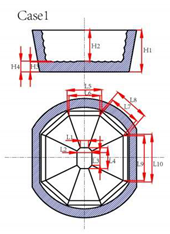 | Height | H1 | mm | 280 |
| H2 | mm | 208 | ||
| H3 | mm | 66 | ||
| H4 | mm | 72 | ||
| Length/Width | L1 | mm | 55 | |
| L2 | mm | 100 | ||
| L3 | mm | 96 | ||
| L4 | mm | 140 | ||
| L5 | mm | 230 | ||
| L6 | mm | 205 | ||
| L7 | mm | 235 | ||
| L8 | mm | 210 | ||
| L9 | mm | 300 | ||
| L10 | mm | 320 | ||
 | Height | H1 | mm | 120 |
| H2 | mm | 325 | ||
| H3 | mm | 380 | ||
| Length/Width | L1 | mm | 375 | |
| L2 | mm | 425 | ||
| L3 | mm | 520 | ||
| L4 | mm | 600 |
| Casting Condition | Unit | Prototype | Model |
|---|---|---|---|
| Inlet flow | L·min−1 | 448.8 | 28.8 |
| Single outlet flow | L·min−1 | 74.8 | 4.8 |
| Height of molten steel | mm | 900 | 300 |
| Inner diameter of ladle shroud | mm | 75 | 25 |
| External diameter of ladle shroud | mm | 130 | 43.3 |
| Submergence depth of ladle shroud | mm | 270 | 90 |
| t | Outlet1 | Outlet2 | Outlet3 | Outlet4 | Outlet5 | Outlet6 | S | E(%) | |
|---|---|---|---|---|---|---|---|---|---|
| case 1 | (s) | 115 | 89 | 88 | 86 | 89 | 114 | 23.54 | 5.87 |
| (s) | 199 | 154 | 152 | 149 | 154 | 197 | |||
| (s) | 188 | 144 | 141 | 141 | 144 | 188 | |||
| case 2 | (s) | 117 | 88 | 84 | 81 | 91 | 123 | 29.98 | 4.17 |
| (s) | 203 | 152 | 145 | 140 | 158 | 213 | |||
| (s) | 199 | 145 | 138 | 138 | 145 | 199 |
© 2020 by the authors. Licensee MDPI, Basel, Switzerland. This article is an open access article distributed under the terms and conditions of the Creative Commons Attribution (CC BY) license (http://creativecommons.org/licenses/by/4.0/).
Share and Cite
Yao, C.; Wang, M.; Zheng, R.; Pan, M.; Rao, J.; Bao, Y. Effect of Turbulence Inhibitors on Molten Steel Flow in 66-Ton T-Type Tundish with Large Impact Area. Metals 2020, 10, 1111. https://doi.org/10.3390/met10091111
Yao C, Wang M, Zheng R, Pan M, Rao J, Bao Y. Effect of Turbulence Inhibitors on Molten Steel Flow in 66-Ton T-Type Tundish with Large Impact Area. Metals. 2020; 10(9):1111. https://doi.org/10.3390/met10091111
Chicago/Turabian StyleYao, Cheng, Min Wang, Ruixuan Zheng, Mingxu Pan, Jinyuan Rao, and Yanping Bao. 2020. "Effect of Turbulence Inhibitors on Molten Steel Flow in 66-Ton T-Type Tundish with Large Impact Area" Metals 10, no. 9: 1111. https://doi.org/10.3390/met10091111