Constitutive Equations for Describing the Warm and Hot Deformation Behavior of 20Cr2Ni4A Alloy Steel

Abstract

Isothermal hot compression tests of 20Cr2Ni4A alloy steel were performed under temperatures of 973–1273 K and strain rates of 0.001–1 s⁻¹. The behavior of the flow stress of 20Cr2Ni4A alloy steel at warm and hot temperatures is complicated because of the influence of the work hardening, the dynamic recovery, and the dynamic recrystallization. Four constitutive equations were used to predict the flow stress of 20Cr2Ni4A alloy steel, including the original strain-compensated Arrhenius-type (osA-type) equation, the new modified strain-compensated Arrhenius-type (msA-type) equation, the original Hensel–Spittel (oHS) equation and the modified Hensel–Spittel (mHS) equation. The msA-type and mHS are developed by revising the deformation temperatures, which can improve prediction accuracy. In addition, we propose a new method of solving the parameters by combining a linear search with multiple linear regression. The new solving method is used to establish the two modified constitutive equations instead of the traditional regression analysis. A comparison of the predicted values based on the four constitutive equations was performed via relative error, average absolute relative error (AARE) and the coefficient of determination (R²). These results show the msA-type and mHS equations are more accurate and efficient in terms of predicting the flow stress of the 20Cr2Ni4A steel at elevated temperature.

1. Introduction

The metal forming process is widely used in the processing of metals and alloys because of its various advantages, including saving of the raw materials, high productivity and premium quality. The metal forming process of alloy steel can be performed under room, warm or hot temperatures. Compared with plastic deformation under room temperature, warm, and hot forming can improve material plasticity and reduce the forming load, due to the temperature raising [1,2].

Generally, the warm forming process is conducted within the temperature range, which is lower than the recrystallization temperature, but higher than the room temperature [3]. The hot forming process is carried out above the recrystallization temperature. When compared with the room and hot forming, warm forming has various advantages, including better surface quality, better grain structure, less subsequent machining and closer tolerances [4,5]. However, the deformation temperature is higher than the recrystallization temperature in the hot forming process. Therefore, the microstructures evolution is more likely to happen, including the dynamic recrystallization, which can realize and achieve such optimum microstructures by controlling their evolution. Moreover, the optimum microstructures can improve the mechanical properties of materials [6,7].

Regarding warm and hot forming, the high-precision constitutive equation can used in the finite element numeric simulation to optimize the forming process and achieve high-efficiency and high-quality production [8].

In past research, many constitutive equations were proposed to predict the flow stress of metals and alloys under elevated temperatures [9,10], which can be summarized into three categories: the empirical, phenomenological and physical models [11]. Moreover, the phenomenological constitutive models have a lesser number of material constants and can be easily calibrated [11].

As a widely used phenomenological model, the strain-compensated Arrhenius-type equation has strong predictive power. Based on the flow stress of Mg–6A1–1Zn alloy, Alireza et al. [12] found the strain-compensated Arrhenius-type equation has a higher prediction accuracy than the Johnson–Cook equation. By considering the FEA application, Wen et al. [13] obtained the same result. A comparative study of Xia et al. [14] suggested the strain-compensated Arrhenius-type equation has a stronger prediction ability than the Johnson–Cook equation and the physically based constitutive equation. To predict the hot flow stress of 10% Cr steel alloy, Abdallah et al. [15] found the prediction accuracy of the strain-compensated Arrhenius-type model is higher than that of modified Johnson–Cook. Moreover, the previous comparative studies have found the strain-compensated Arrhenius-type equation can give a more accurate description of the relationship between flow stress and deformation conditions when compared with the modified Johnson–Cook, Johnson–Cook equations [16,17]. Moreover, based on the stress–strain data of T24 steel, a comparative study of Li et al. [18] showed the predictability of the strain-compensated Arrhenius-type equation is stronger than that of the modified Zerilli–Armstrong equation. The results from earlier comparative studies demonstrated the strain-compensated Arrhenius-type equation can predict flow stress more accurately via comparing with the modified Zerilli–Armstrong and Johnson–Cook equations [19,20,21]. In addition, based on flow stress curves of the powder metallurgy tungsten, Wang et al. [22] found the strain-compensated Arrhenius-type equation had the highest accuracy when compared to the Johnson–Cook, modified Johnson–Cook, Zerilli–Armstrong, modified Zerilli–Armstrong and KHL equations. A number of the above studies have identified that the strain-compensated Arrhenius-type equation has higher prediction accuracy. Therefore, the strain-compensated Arrhenius-type equation with a higher prediction accuracy is widely used to predict the flow stress of metals and alloys [23,24,25].

In addition, Hensel and Spittel (1978) proposed a constitutive equation (namely Hensel–Spittel equation) for the description of the rigid-plastic material flow stress [26]. El Mehtedi et al. [27] used the Hensel–Spittel equation to predict the flow stress of wrought aluminum alloys. Moreover, the Hensel–Spittel equation can be used to describe the relationship between strain, strain rates, temperatures and stress based on the 6061 aluminum alloy, the Mg–9Li–3Al–2Sr–2Y alloy, the TiAl–Mo alloys, HSLA350/440 and DP350/600 steels [28,29,30,31]. Moreover, based on the hot tensile deformation of Ti–6Al–4V Alloy, the Hensel–Spittel equation has a higher prediction accuracy than the strain-compensated Arrhenius-type equation [32].

20Cr2Ni4A steel is a kind of representative high-strength alloy carburizing steel which has superior comprehensive mechanical properties, such as prominent hardenability and durability [33,34]. Therefore, 20Cr2Ni4A steel is widely applied to produce broad cross-section carburized parts. In previous research, there are many reports about the constitutive equation of metals and alloys at warm or hot temperatures [35,36,37,38,39]. The aim of the present study is that a higher-precision constitutive equation is established to describe the behavior of the 20Cr2Ni4A steel under a wider range, including warm forming and hot forming.

In the current study, the isothermal hot compression tests of the 20Cr2Ni4A alloy steel were carried out at the deformation temperature ranging from 973.15 K to 1273.15 K. The four constitutive equations are established to describe the deformation behavior of the 20Cr2Ni4A alloy steel under warm and hot temperature, including the original strain-compensated Arrhenius-type (osA-type) equation, the original Hensel–Spittel (oHS) equation, the new modified strain-compensated Arrhenius-type (osA-type) equation and the new modified Hensel–Spittel (mHS) equation. The new modified strain-compensated Arrhenius-type equation and the new modified Hensel–Spittel equation are established by revising the deformation temperatures over the entire range of deformation conditions. In addition, the new method is proposed to establish the above two modified constitutive equations. Moreover, the new method can combine multiple regression analysis with a linear search to determine the parameters in constitutive equations.

A comparative study is made to find a suitable constitutive equation to describe the warm and hot deforming behavior of the 20Cr2Ni4A alloy steel.

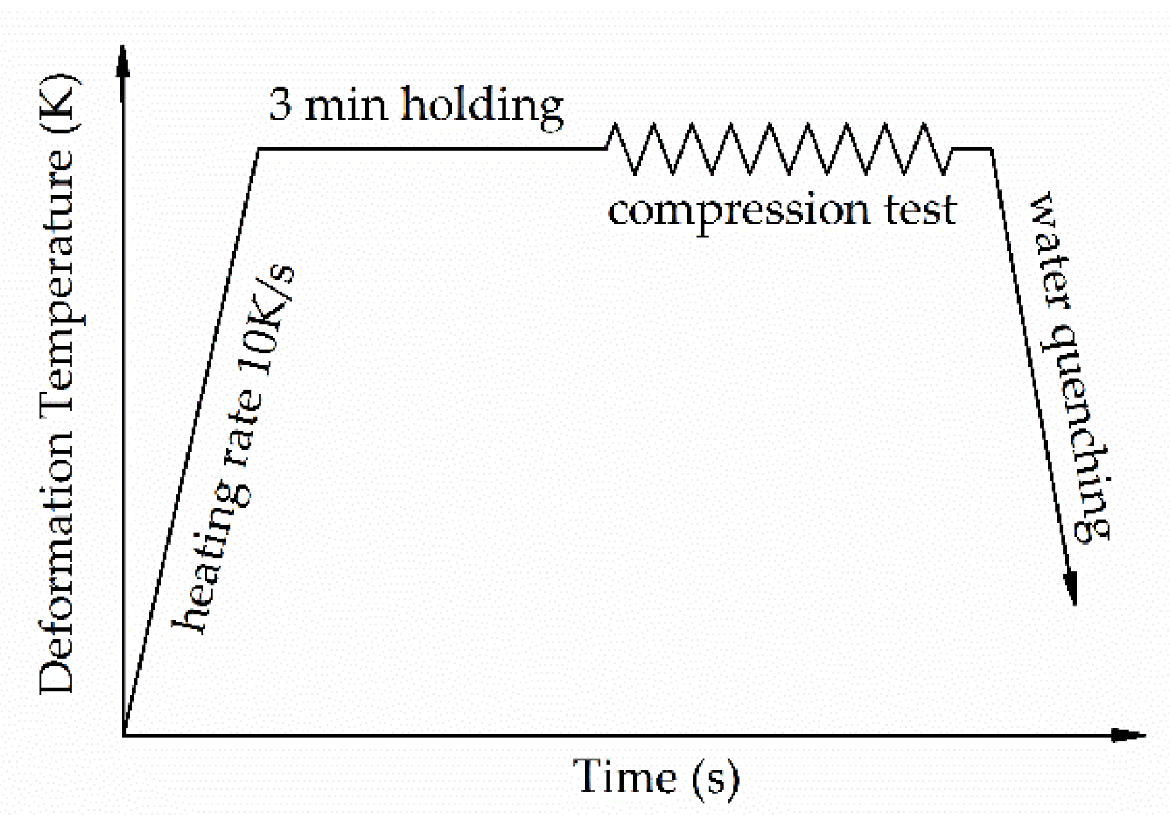
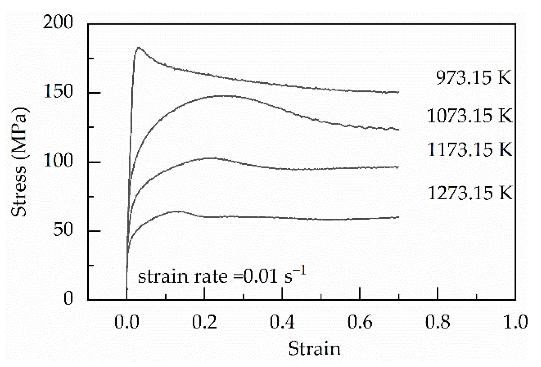
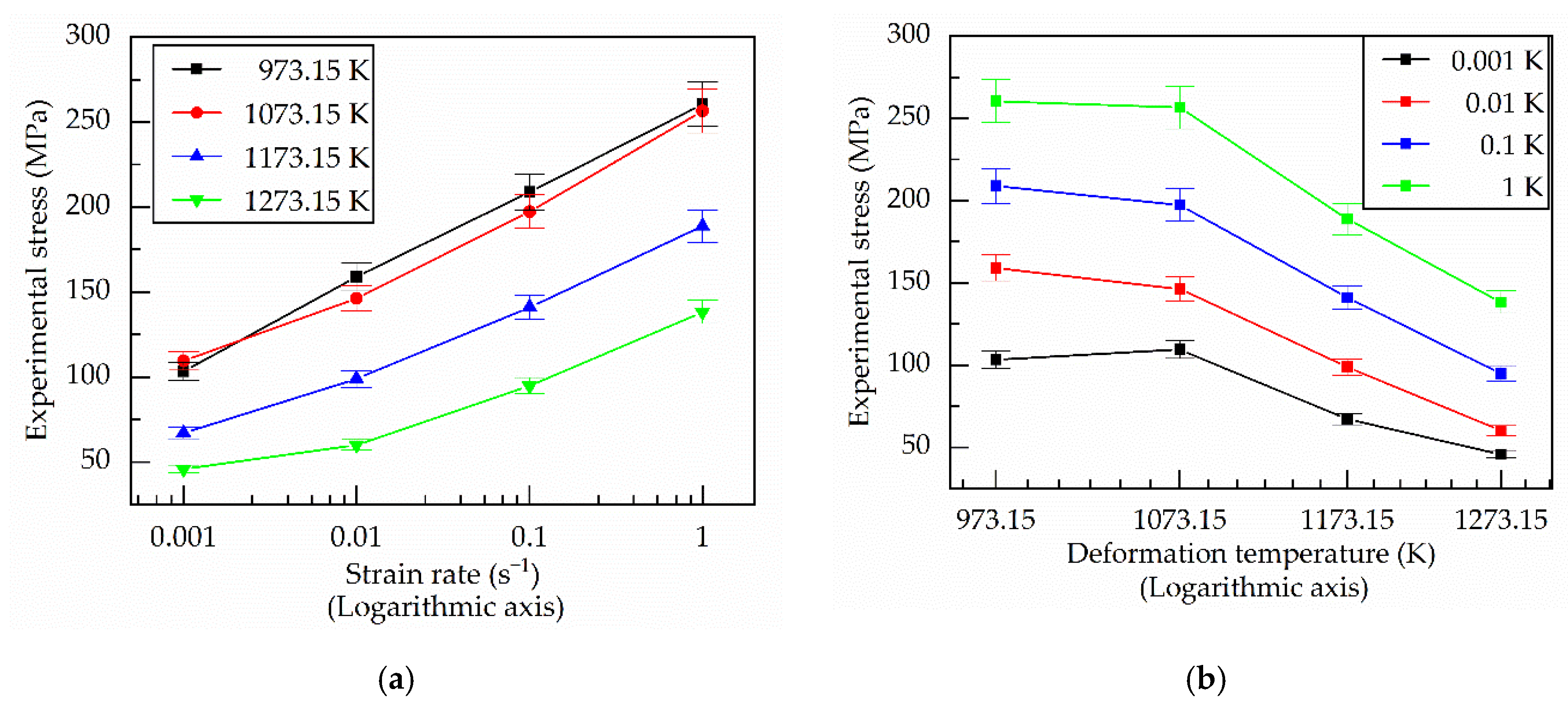
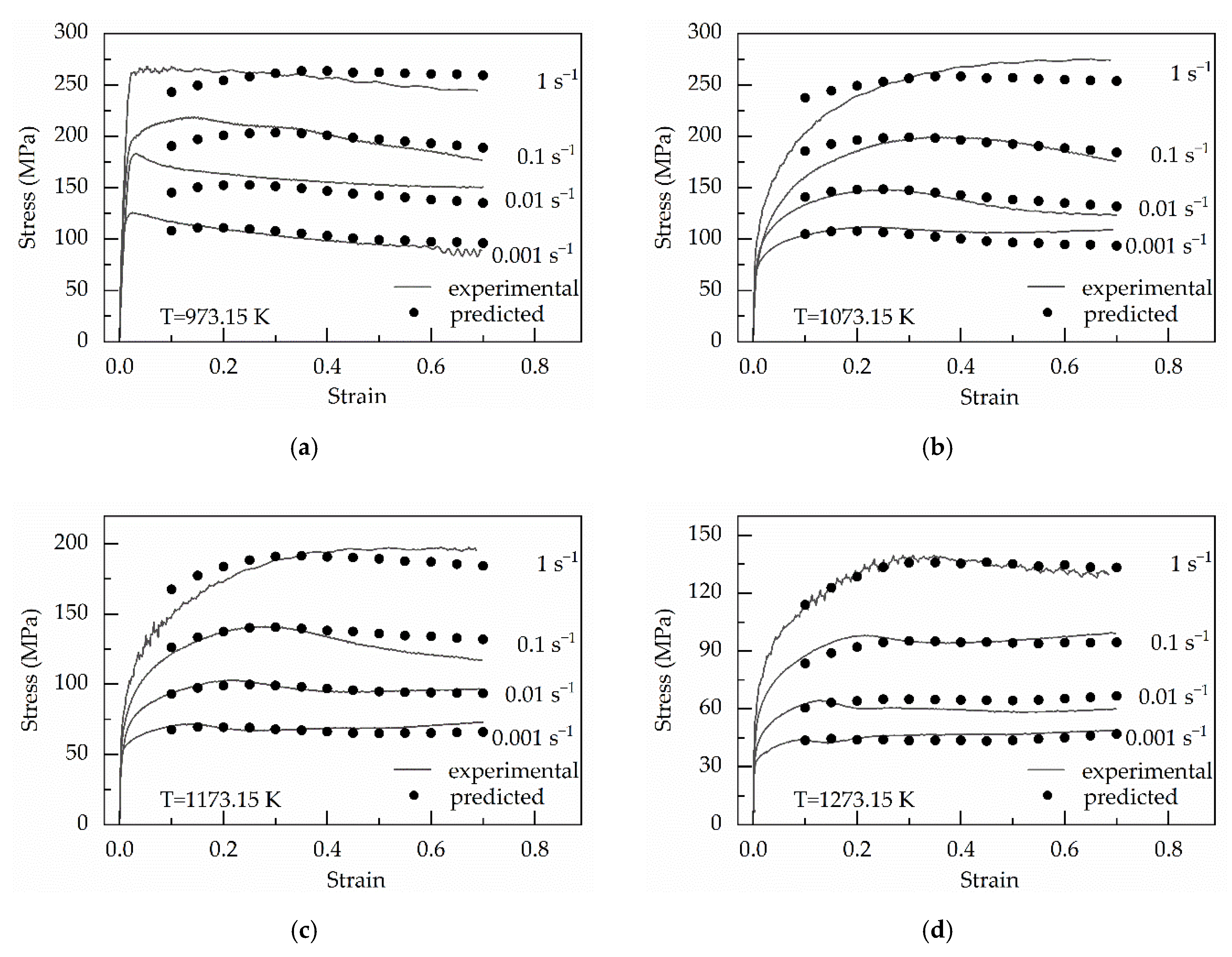
2. Experimental Procedure and Results

The material used in this research was 20Cr2Ni4A alloy steel, whose chemical composition is shown in

Table 1. Chemical component of 20Cr2Ni4A alloy steel.

Parameter	C	Si	Mn	Cr	Ni	S	P	Fe
Value (%)	0.19	0.21	0.45	1.55	3.24	0.002	0.005	Bal

. The isothermal hot compression tests were carried out on the Gleeble-3500 simulator (Dynamic Systems, Inc., Poestenkill, NY, USA) at the deformation temperature ranging from 973.15 K to 1273.15 K with an increment of 100 K, the strain rated of 0.001, 0.01, 0.1 and 1 s⁻¹. Cylindrical specimens 12 mm in height and 8 mm in diameter were prepared. Each flat end of the specimen was covered with the tantalum foil to minimize friction. The flow chart of the isothermal hot compression was shown in Figure 1. Each specimen was heated to the deformation temperature at 10 K/s and then held for 3 min to equilibrate the temperature throughout the specimen. Next, the specimens were compressed up to true strain of 0.70. After that, they were immediately water quenched.

During the warm and hot forming process, the plastic flow behavior of metals and alloys is dependent on the equilibrium between the work hardening and the dynamic softening mechanisms [40]. However, there are different dynamic softening mechanisms in the warm and hot forming process. In the warm forming process, the dynamic softening mechanism is mainly the dynamic recovery [41,42]. In the hot forming process, the dynamic softening mechanisms involve the dynamic recovery and dynamic recrystallizations [43].

At the early stage of the warm and hot forming process, there was the same plastic flow behavior due to work hardening. Namely, the stress increases sharply because of the rapidly increasing dislocation density and the limited dynamic softening mechanisms [43,44].

Next, the stress increased slowly until it reaches the peak stress, where there were the different true strain corresponding to the peak stress with increasing the temperature. For example, the strain corresponding to the peak stress at 973.15 K was lower than the strain corresponding to the peak stress at 1073.15 K in Figure 2. The reason was that, in the warm forming process, increasing the forming temperatures would lower the critical shear stress of materials and promote the cross-slip and climb of dislocation. Dynamic recovery is mainly achieved through the cross-slip and climb of dislocation [5]. Thus, as the deformation temperature increases, the critical strain required for dynamic recrystallization decreases [5]. At 973.15 K, because the critical strain required for dynamic recrystallization was higher, at the early stage, the work hardening made dislocation density and stress higher. When strain reached the critical strain required for dynamic recrystallization, the softening rate of the dynamic softening mechanisms was higher than the work hardening rate because the higher dislocation density promoted dynamic recrystallization. Therefore, after reaching the peak stress, true stress began to decrease sharply. As strain increased, the softening rate of the dynamic softening mechanisms decreased due to decreasing dislocation density. Finally, it was achieved the equilibrium between the work hardening and the dynamic softening mechanisms. Therefore, at 973.15 K, the flow stress curve after the peak stress was a concave curve.

At 1073.15 K, the critical strain required for dynamic recrystallization was relatively lower. When strain reaches the critical strain required for dynamic recrystallization, the softening rate was lower than the hardening rate because of the lower dislocation density. As strain increased, the work hardening increased dislocation density because the hardening rate was higher than the softening rate. Moreover, because the increase of the dislocation density promotes dynamic recrystallization, the change in the softening rate gradually approaches the hardening rate. Finally, an equilibrium between the work hardening and the dynamic softening mechanisms was achieved, and stress reached a peak. Therefore, at 1073.15 K, the flow-stress curve before the peak stress was convex. In addition, the strain corresponding to the peak stress at 1073.15 K was higher than the strain corresponding to the peak stress at 973.15 K.

In contrast, for instance, the strain corresponding to the peak stress at the temperature of 1073.15 K, 1173.15 K and 1273.15 K decreased in turn in Figure 2. The reason was that, in the hot forming process, the high temperature promotes the nucleation and growth of dynamically recrystallized grains and dislocation annihilation [45,46]. Namely, raising the deformation temperature further enhanced the softening mechanism and weakened work hardening, so the peak stress advanced [43].

Subsequently, the flow stress decreased steeply because the dynamic softening mechanisms become predominant. Finally, the flow curves exhibit a steady stage duo to a new balance between softening and hardening [3,43]. In summary, the deformation temperature was an important influencing factor that caused the difference between flow-stress curves.

Figure 3a shows the relationship between flow stress and strain rates under different deformation temperatures and strain of 0.30. It is easily found that there was an approximately linear relationship between flow stress and strain rates under different deformation temperatures. Figure 3b shows the relationship between flow stress and deformation temperatures under different strain rates and strain of 0.30. As deformation temperatures increase from 973.15 to 1073.15 K, the change in stress value was small at the same strain rate because the impact of the dynamic softening mechanisms was very limited below the dynamic recrystallization temperature. When the deformation temperature was higher than 1073.15 K, the stress decreased as with the rise of deformation temperatures. The reason for the reduction in stress was that the dynamic softening mechanisms become increasingly sufficient due to the increase in temperature. Based on the analysis of Figure 3, it was easily found the changing trend of stress was mainly affected by deformation temperatures, and there was a relatively complex nonlinear relationship between the stress and deformation temperatures.

3. Constitutive Equation

Based on the above analysis, the deformation temperature is the main factor in the changing trend of stress and the relationship between the deformation temperature and the flow stress is complicated. Therefore, a higher precision constitutive equation may be established by revising the deformation temperature in the existing constitutive equation. Two modified constitutive equations were developed, namely the modified strain-compensated Arrhenius-type (msA-type) equation and the modified Hensel–Spittel (mHS) constitutive equation. In addition, the original strain-compensated Arrhenius-type (osA-type) equation and the original Hensel–Spittel (oHS) constitutive equation were also established. The four constitutive equations were used to try to develop a higher precision constitutive equation for the 20Cr2Ni4A steel under the warm forming and the hot forming.

3.1. The Original Strain-Compensated Arrhenius-Type (osA-type) Equation

The Arrhenius-type equation is shown in Equation (1). The common effect of the temperatures and strain rates on the hot deformation behavior can be seen through the Zener–Hollomon parameter (Z) in an exponent-type equation, which is shown in Equation (2) [38]:

$$\dot{\epsilon }=\mathrm{AF}(\sigma )\exp (-\mathrm{Q}/(\mathrm{RT}))$$

(1)

$$Z=\dot{\epsilon }\exp (\mathrm{Q}/(\mathrm{RT}))$$

(2)

where

$$F(\sigma )=\{\begin{array}{l}{\sigma }^{n_1}(\alpha \sigma <0.8)\\ \exp (\beta \sigma )(\alpha \sigma >1.2)\\ {[\sinh (\alpha \sigma )]}^n(forall\sigma )\end{array}$$

(3)

where $\dot{\epsilon }$ is the real strain rate (s⁻¹), σ is the flow stress (MPa), T is the deformation temperature (K), Q is the activation energy (J·mol⁻¹), R is the molar gas constant (8.3145 J·mol⁻¹·K⁻¹), A, n₁, n, α and β are material constants.

Regarding the original Arrhenius-type equation, it has been proposed by Sellars and Tegart [35] that a hyperbolic sine-type equation can be employed to correlate the saturation stress to the deformation conditions over a very wide range of stress, which is shown in Equation (4).

$$\dot{\epsilon }=\mathrm{A}{[\sinh (\alpha \sigma )]}^n\exp (-\mathrm{Q}/(\mathrm{RT}))$$

(4)

The hyperbolic sine function sinh(ασ) is described with Taylor series expansion as:

$$\sinh (\alpha \sigma )=\alpha \sigma +\frac{{(\alpha \sigma )}^n}{3!}+\frac{{(\alpha \sigma )}^n}{5!}+\frac{{(\alpha \sigma )}^n}{7!}+\cdots$$

(5)

When ασ is small, the above term that is more than third power have very small values, which can be ignored, thus, sinh(ασ) ≈ ασ. In contrast, if ασ is large, the value of the item $e^{-\alpha \sigma }$ can be ignored, which leads to sinh(ασ) ≈ $e^{\alpha \sigma }$/2.

Based on the above analysis, Equation (4) can be simplified as:

$$\{\begin{array}{ll}\dot{\epsilon }={\mathrm{A}}_1{\sigma }^n\exp (-\mathrm{Q}/(\mathrm{RT}))& \mathrm{when}\alpha \sigma \mathrm{smaller}\\ \dot{\epsilon }={\mathrm{A}}_2\exp (\alpha n\sigma )\exp (-\mathrm{Q}/(\mathrm{RT}))& \mathrm{when}\alpha \sigma \mathrm{larger}\end{array}$$

(6)

where A₁ = A${\alpha }^n$, A₁ = A$/2^n$, n ≈ n₁ and an ≈ β. Therefore, the material constant α is obtained based on Equation (7) [47].

$$\alpha \approx n_1/\beta$$

(7)

In summary, the hyperbolic sine in the Arrhenius-type equation can predict flow stress over a very wide range of stress.

Currently, Equation (7) is still used to solve the value of the material constant α. However, the method of solving α is approximate. Therefore, in previous research, the material constant α was used as an adjustable parameter to improve the prediction accuracy of the Arrhenius-type equation [48,49,50]. However, no simple method has been proposed to determine α-value. Therefore, it is not widely used that the material constant α is used as an adjustable parameter. In the present study, the material constant α is still determined based on Equation (7). Moreover, the hyperbolic sine in the Arrhenius-type equation (namely, Equation (4)) is used to predict the flow stress of 20Cr2Ni4A alloy steel. Because there is no strain in Equation (4), the polynomial in strain and material constants is employed to represent the influence of strain on stress to establish the strain-compensated Arrhenius-type equation [10].

3.2. The Modified Strain-Compensated Arrhenius-Type (msA-type) Equation

The hyperbolic sine law in Arrhenius-type model can provide a better description of the relationship between strain rates, deformation temperatures and flow stress. Therefore, based on the hyperbolic sine law, the new modified constitutive model is established by introducing the new variable T* into Arrhenius-type model, which is shown in Equation (8):

$$\dot{\epsilon }=\mathrm{A}\left[\sinh \right(\alpha \sigma {\left)\right]}^n\exp (-\frac{\mathrm{Q}}{{\mathrm{RT}}^{*}})$$

(8)

where $\dot{\epsilon }$ is the strain rate (s⁻¹), σ is the flow stress (MPa), T* is the equivalent temperature (K), Q is the activation energy (J·mol⁻¹), R is the molar gas constant (8.314 J·mol⁻¹ K⁻¹), A, n and α are material constants. Moreover, T* is a function of the deformation temperature T.

Because T* is a function of the deformation temperature T, the introduction of new variable T* means to revising the relationship between the deformation temperature and the flow stress. Namely, the relationship between T and σ described by the original constitutive equation is reestablished. Based on the analysis of Section 2, the deformation temperature is the main factor. Therefore, the prediction accuracy of constitutive equations can be improved by revising the deformation temperature.

Although Peng et al. [51] applied the trial and error method to modify the deformation temperature, it is not widely used due to the disadvantages of the trial and error method.

Therefore, in the present study, it is introduced the new method combines multiple regression analysis with a linear search, which can be used to determine more reasonable values of material constants and revise the deformation temperature. For example, the new method can be used to solve the material constant α instead of Equation (7). In addition, as a widely used optimization algorithm, a linear search is easier to obtain more reasonable values of material constants when compared with trial and error method.

In the modified strain-compensated Arrhenius-type equation, the polynomial was employed to represent the influence of strain on stress.

3.3. The Original Hensel–Spittel (oHS) Equation

Hensel and Spittel developed a constitutive equation (namely the Hensel–Spittel (oHS) equation) to describe the deformation behavior of alloy at high temperature [26]. The oHS equation is shown in Equation (9):

$$\sinh (\alpha \sigma )=\mathrm{A}\exp (m_1\mathrm{T}){\epsilon }^{m_2}{\dot{\epsilon }}^{m_3}\exp (m_4/\epsilon ){(1+\epsilon )}^{m_5\mathrm{T}}\exp (m_6\epsilon ){\dot{\epsilon }}^{m_7\mathrm{T}}{\mathrm{T}}^{m_8}$$

(9)

where σ is stress, ε is strain, $\dot{\epsilon }$ is strain rate, T is the deformation temperature, A, m₁, m₂, m₃, m₄, m₅, m₆, m₇ and m₈ are material parameters. m₁ and m₈ define the material’s sensitivity to temperature, m₅ defines coupling temperature and strain, m₇ term coupling temperature and strain rate, m₂, m₄ and m₆ define the material’s sensitivity to strain and m₃ depends on the material’s sensitivity to strain rate. To simplify Equation (34), it was assumed that, at a given strain (or at steady state), the stress exponent n = 1/(m₃ + m₇ T) should be temperature independent, i.e., m₇ = 0 [27]. Moreover, both m₁ and m₈ are related to the deformation temperature [29]. Therefore, constants m₇ and m₈ are usually taken as zero. The material parameter α in Equation (9) can be determined by the polynomial in α and strain of the original strain-compensated Arrhenius-type equation [32].

3.4. The Modified Hensel–Spittel (mHS) Equation

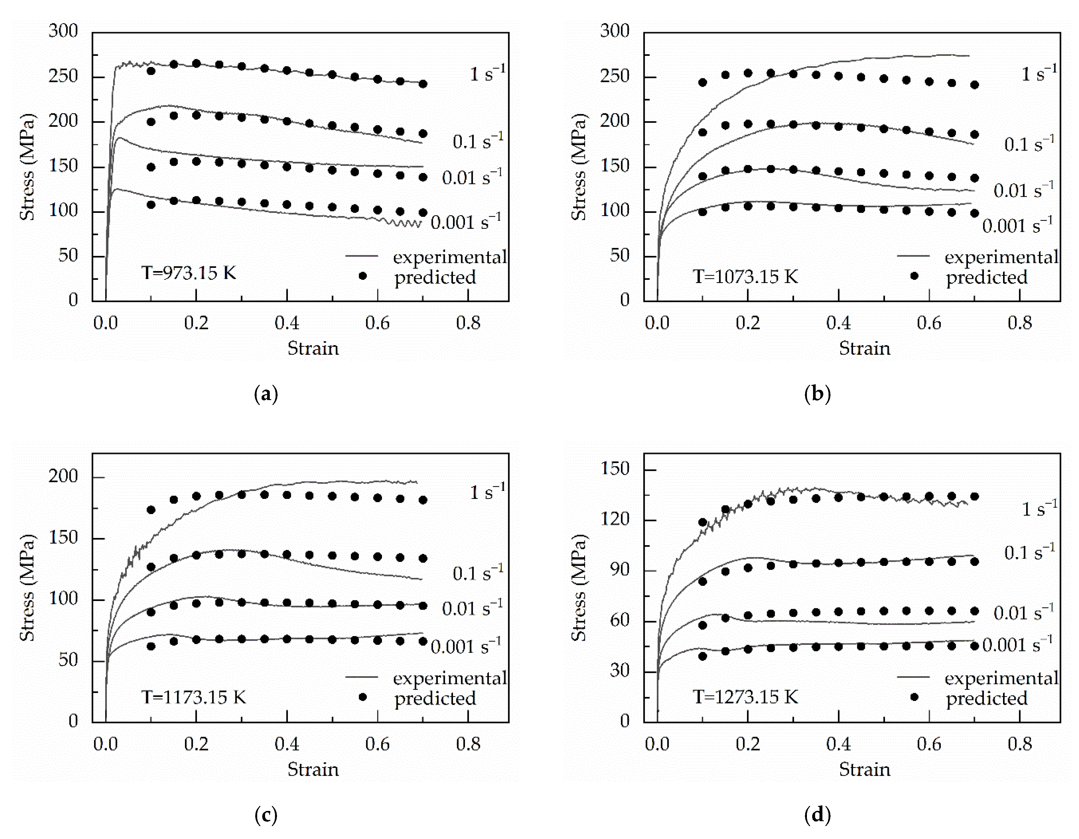
A modified Hensel–Spittel constitutive equation was also developed by revising the deformation temperature, which is shown Equation (10).

$$\sinh (\alpha \sigma )=\mathrm{A}\exp (m_1{\mathrm{T}}^{*}){\epsilon }^{m_2}{\dot{\epsilon }}^{m_3}\exp (m_4/\epsilon ){(1+\epsilon )}^{m_5{\mathrm{T}}^{*}}\exp (m_6\epsilon ){\dot{\epsilon }}^{m_7{\mathrm{T}}^{*}}{\left({\mathrm{T}}^{*}\right)}^{m_8}$$

(10)

where A, m₁, m₂, m₃, m₄, m₅, m₆, m₇ and m₈ are still material parameters. Moreover, m₇ and m₈ are still neglected. T* is the equivalent temperature, which is still a function of the deformation temperature T. However, the material parameter α in Equation (10) is a fixed value independent of strain. Similarly, the new method, which combines multiple regression analysis with a line search method, can be used to determine the material parameters and revise the deformation temperatures.

4. Results

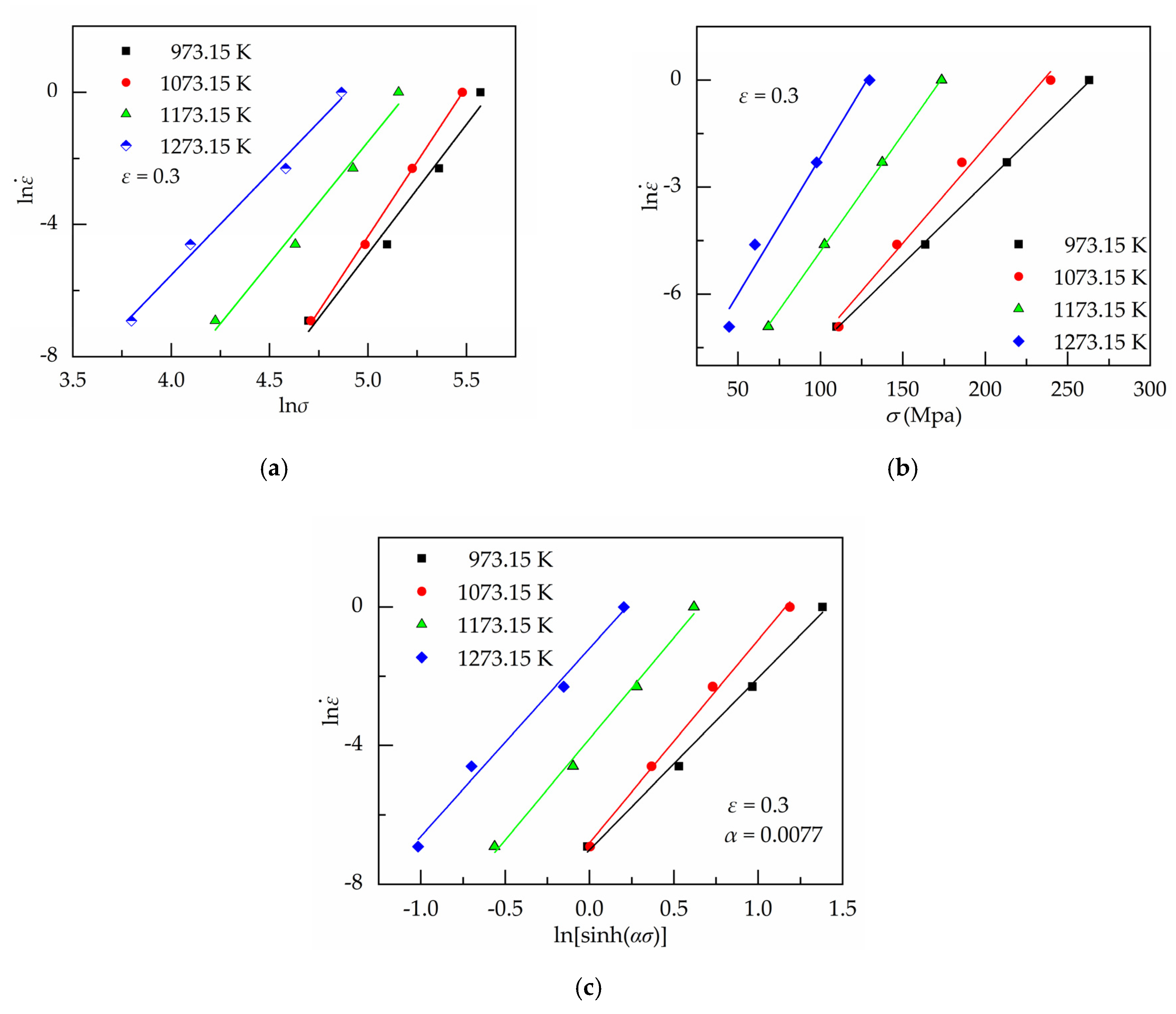
4.1. Establishing the Original Strain-Compensated Arrhenius-Type (osA-type) Equation

Regarding the original strain-compensated Arrhenius-type equation, the procedure of determining material constants for a special true strain is as follows. A strain of 0.30 is taken as an example.

Taking Equation (3), substituting the power law, the exponential law and the hyperbolic sine law of F (σ) into Equation (1) and then taking logarithm from both sides of the equations yields:

$$\ln \dot{\epsilon }=\ln \mathrm{A}+n_1\ln \sigma -\mathrm{Q}/(\mathrm{RT})$$

(11)

$$\ln \dot{\epsilon }=\ln \mathrm{A}+\beta \sigma -\mathrm{Q}/(\mathrm{RT})$$

(12)

$$\ln \dot{\epsilon }=n\ln \left[\sinh \right(\alpha \sigma \left)\right]+\ln \mathrm{A}-\mathrm{Q}/(\mathrm{RT})$$

(13)

By the linear regression analysis based on Equations (11) and (12), the n₁-value and β-value can be determined from the mean value of the slope of the lines in lnσ vs. ln$\dot{\epsilon }$ and σ vs. ln$\dot{\epsilon }$ plots, respectively, as shown in Figure 4a,b. The α-value is equal to 0.0077 MPa⁻¹ based on Equation (7). In addition, based on Equation (13), the n-value can be obtained from the mean value of the slope of the lines in ln[sinh(ασ)] vs. ln$\dot{\epsilon }$ plots, as shown in Figure 4c.

Differentiating Equation (13) gives:

$$\mathrm{Q}=\mathrm{R}n\frac{\partial \ln \left[\sinh \right(\alpha \sigma \left)\right]}{\partial (1/\mathrm{T})}$$

(14)

Therefore, Q-value is calculated by averaging the slopes of 1000/T vs. ln[sinh(ασ)] under different strain rates in Figure 5a.

Substituting Equation (2) and the hyperbolic sine law of F (σ) into Equation (1) yields:

$$Z=\mathrm{A}{[(\sinh (\alpha \sigma ))]}^n$$

(15)

Taking the logarithm of both sides of Equation (15) gives:

$$\ln Z=\ln \mathrm{A}+n[\ln (\sinh (\alpha \sigma ))]$$

(16)

After gaining the values of α, n and Q, the value of lnA can be deduced from the intercept of ln[sinh(ασ)]-lnZ curve, as shown in Figure 5b.

In summary, it is obtained the material constant α, n, Q and A under the strain of 0.30. However, when the value of strain is different, the values of the material constant α, n, Q and A will change. For establishing the strain-compensated Arrhenius-type (osA-type) equation, the value of the strain ranges from 0.10 to 0.70 at an interval of 0.05. By repeating the above process, it is determined the material constants under different strain. The polynomial is employed to describe the relationship between material parameters and strain [36]. By adjusting the order of the polynomial, it is found one fifth-order polynomial fitting can obtain a very good correlation and generalization, which is shown in Equation (18) and Figure 6 [36].

Table 2. Coefficients of the polynomial for α, n, Q and lnA in the osA-type equation.

α (MPa−1)	n	Q (kJ·mol−1)	lnA
α0 = 0.0099	N0 = 8.1874	Q0 = 441.1503	A0 = 42.0394
α1 = −0.0159	N1 = −26.3749	Q1 = −2274.7592	A1 = −239.5653
α2 = 0.0330	N2 = 97.1817	Q2 = 8516.0320	A2 = 915.6306
α3 = −0.0012	N3 = −199.2349	Q3 = −16,792.012	A3 = −1834.8319
α4 = −0.0638	N4 = 214.8862	Q4 = 16,706.7723	A4 = 1847.7995
α5 = 0.0463	N5 = −92.8376	Q5 = −6637.2152	A5 = −740.3887

shows coefficients of the polynomial for α, n, Q and lnA in the osA-type equation. After determining material parameters under different strains, the predicted stress can be determined based on Equation (17), which is shown in Figure 7.

$$\{\begin{array}{l}\sigma =\frac{1}{\alpha }\ln \left\{{\left(\frac{Z}{A}\right)}^{1/n}+{\left[{\left(\frac{Z}{A}\right)}^{2/n}+1\right]}^{1/2}\right\}\\ Z=\dot{\epsilon }\exp [\mathrm{Q}/(\mathrm{RT})]\hfill \end{array}$$

(17)

$$\{\begin{array}{l}\alpha =a_0+a_1\epsilon +a_2{\epsilon }^2+a_3{\epsilon }^3+a_4{\epsilon }^4+a_5{\epsilon }^5+a_6{\epsilon }^6+a_7{\epsilon }^7\\ n=N_0+N_1\epsilon +N_2{\epsilon }^2+N_3{\epsilon }^3+N_4{\epsilon }^4+N_5{\epsilon }^5+N_6{\epsilon }^6+N_7{\epsilon }^7\\ \mathrm{Q}={\mathrm{Q}}_0+{\mathrm{Q}}_1\epsilon +{\mathrm{Q}}_2{\epsilon }^2+{\mathrm{Q}}_3{\epsilon }^3+{\mathrm{Q}}_4{\epsilon }^4+{\mathrm{Q}}_5{\epsilon }^5+{\mathrm{Q}}_6{\epsilon }^6+{\mathrm{Q}}_7{\epsilon }^7\\ \ln A=A_0+A_1\epsilon +A_2{\epsilon }^2+A_3{\epsilon }^3+A_4{\epsilon }^4+A_5{\epsilon }^5+A_6{\epsilon }^6+A_7{\epsilon }^7\end{array}$$

(18)

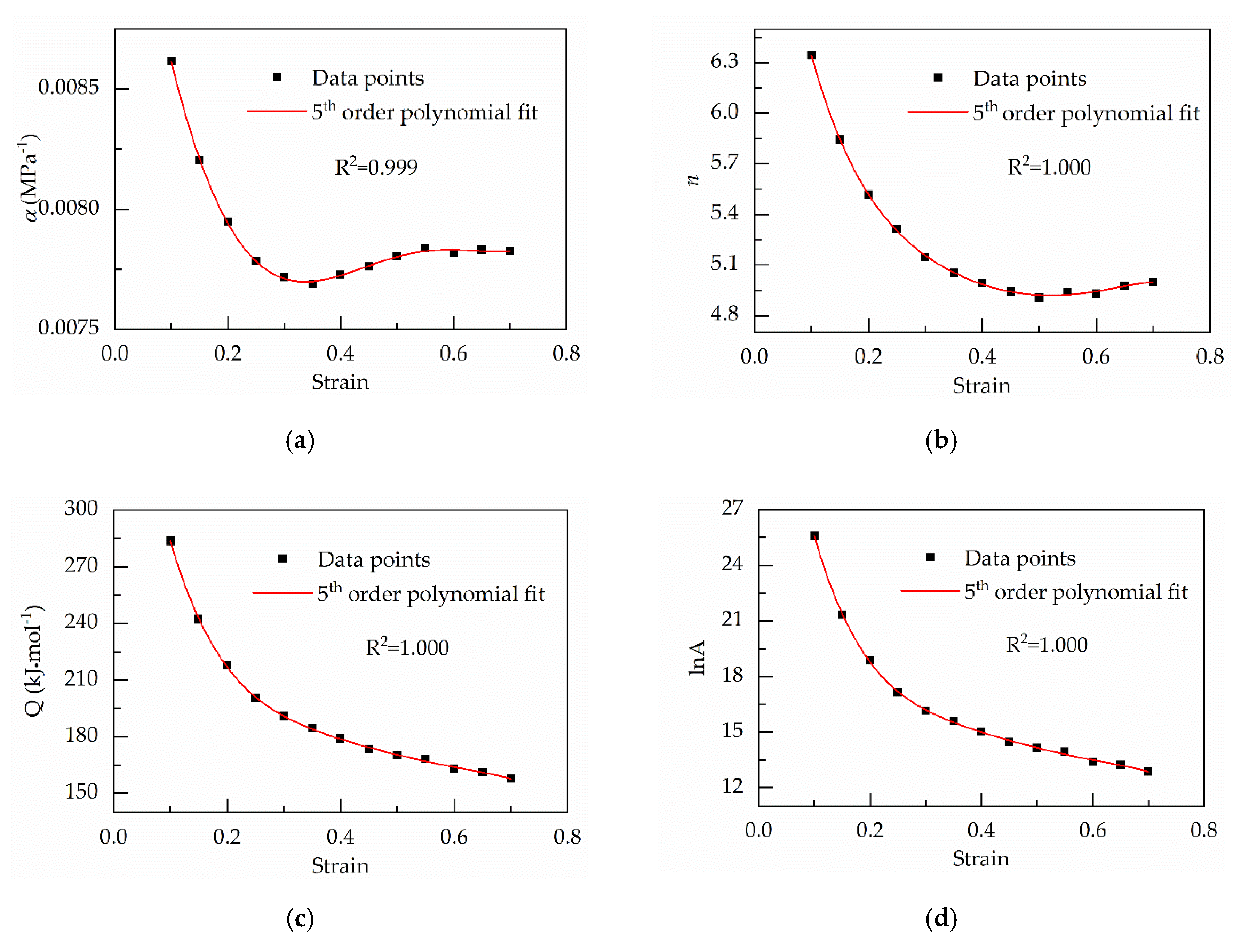
4.2. Establishing the Modified Strain-Compensated Arrhenius-Type (msA-type) Equation

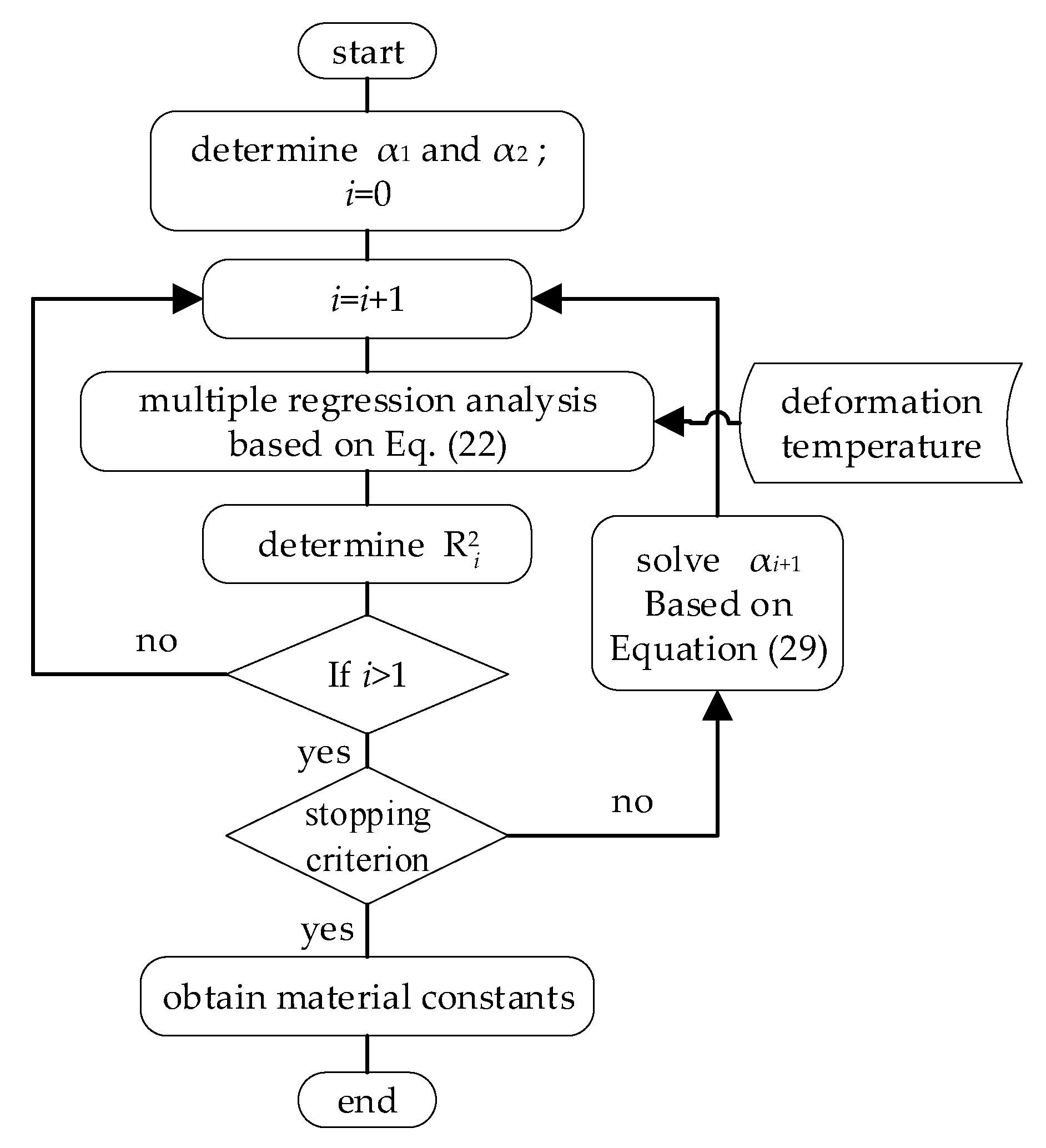
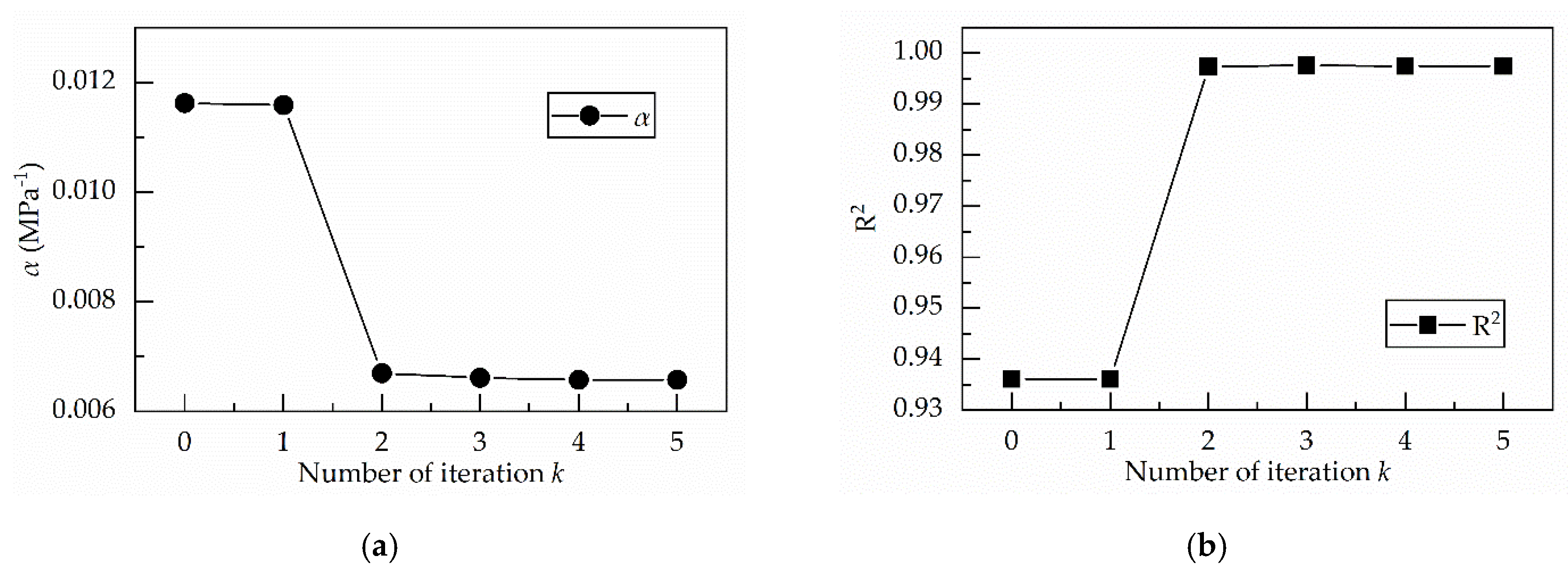
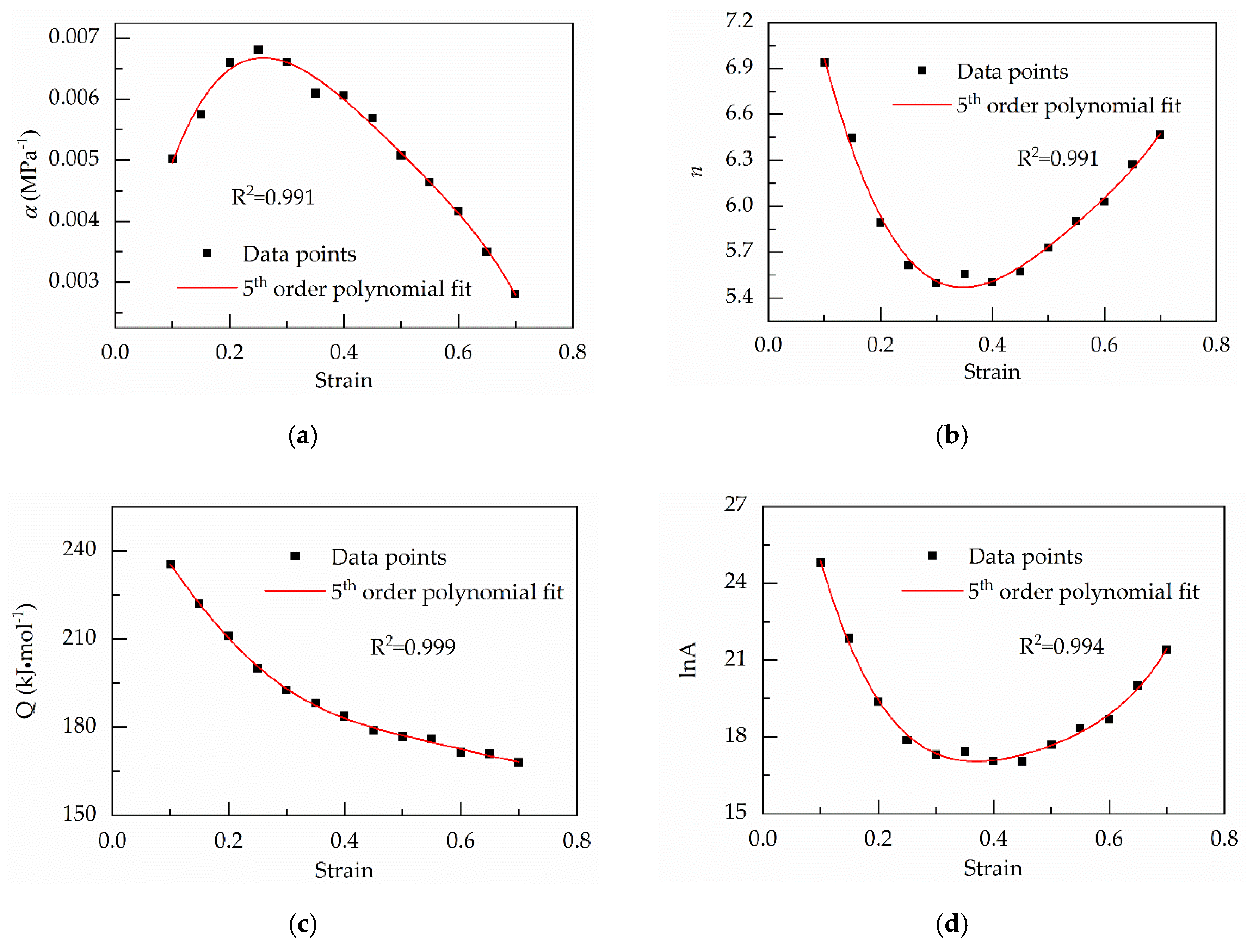
4.2.1. Solving the Material Constants

Regarding the modified strain-compensated Arrhenius-type (msA-type) equation, first, it is determined the values of the material constants A, n, m and α. Then the equivalent temperature is obtained based on the material constants under different strain. Under a single strain, the material constants A, n, m and α will be calculated by the new method, which combines multiple regression analysis with a line search method. During determining the material constants, the deformation temperature is used instead of the equivalent temperature, which is shown in Equation (19):

$$\dot{\epsilon }=\mathrm{A}\left[\sinh \right(\alpha \sigma {\left)\right]}^n\exp (-\frac{\mathrm{Q}}{\mathrm{RT}})$$

(19)

The process of solving the material constants under a single strain is as follows: Taking the logarithm of both sides of Equation (19) gives:

$$\ln \dot{\epsilon }=\ln (\mathrm{A})+n\ln \left[\sinh \right(\alpha \sigma \left)\right]-\mathrm{Q}\times \frac{1}{\mathrm{RT}}$$

(20)

Based on Equation (20), Equation (21) is established:

$$\{\begin{array}{l}y=\ln \dot{\epsilon }\\ x_1=\ln [\sinh (\alpha \sigma )]\\ x_2={10}^3/(\mathrm{RT})\\ b_1=n\\ b_2=\mathrm{Q}\\ b_3=\ln (\mathrm{A})\end{array}$$

(21)

where the unit of Q becomes kJ·mol⁻¹. Because the value of 1/(RT) is relatively smaller, the 1000/(RT) is used instead of 1/(RT) to improve the calculation accuracy.

Substituting Equation (21) in Equation (20) yields:

$$y=b_1{x}_1+b_2{x}_2+b_3$$

(22)

After determining α-value, the vales of y, x₁ and x₂ (namely, ln$\dot{\epsilon }$, ln[sinh(ασ)] and 10³/(RT)) are calibrated based on experimental data. However, the values of b₁, b₂ and b₃ (namely, n, Q and ln(A)) are still unknown. Therefore, Equation (22) can be used as a linear regression model, where x₁ and x₂ are the independent variables, y₁ is the dependent variable and b₁, b₂ and b₃ are the unknown parameters.

When α-value is determined, the values of b₁, b₂ and b₃ can be calculated by regression analysis. However, the α-value will directly influence the results of regression analysis and the predicted stress obtained based on the constitutive equation.

The coefficient of determination (R²) is a measure used in statistical analysis, which assesses how well a model explains, as shown in Equation (23):

$${\mathrm{R}}^2=1-\frac{{\displaystyle \sum _{i=1}^N{(E_i-P_i)}^2}}{{\displaystyle \sum _{i=1}^N{(E_i-\overline{E})}^2}}$$

(23)

where E_i is the experimental data, P_i is the predicted value obtained from the constitutive equation, Ē is the mean value of E_i and N is the total number of data employed in the investigation. Under a single strain, there are 4 different deformation temperatures (973.15, 1073.15, 1173.15 and 1273.15 K) and 4 different strain rates (0.001, 0.01, 0.01 and 1 s⁻¹). Therefore, there are 16 different data points selected, namely, N = 16.

In addition, average absolute relative error (AARE) is an unbiased statistical parameter that is calculated via a term-by-term comparison of the relative error [13], as shown in Equation (24). Moreover, AARE is always used to verify the accuracy of the constitutive models.

$$\mathrm{AARE}(\%)=\frac{1}{N}{\displaystyle \sum _{i=1}^{N_i}\frac{|E_i-P_i|}{E_i}}\times 100$$

(24)

where E_i is the experimental data, P_i is the predicted value obtained from the constitutive equation, and N is the total number of data points employed in the investigation. Similarly, N is 16 when AARE is used to solve material constants under a single strain.

It is assumed the predicted stress σ_p is equal to the experimental stress σ_e over the entire range of deformation conditions, namely the equation σ_p = σ_e holds. There is a linear relationship between the predicted stress and experimental stress. R² is used in statistics to measure how strong a linear relationship is between two variables.

When the equation σ_p = σ_e holds, it is obtained the highest prediction accuracy, and R²-value is one. When σ_p is not equal to σ_e under some conditions, the linear relationship between σ_p and σ_e becomes weaker. With increasing the difference between σ_p and σ_e, the linear relationship between σ_p and σ_e keep getting weaker. Moreover, R²-value and the prediction accuracy continuously decrease. Meanwhile, the AARE value continuously increases.

Therefore, both R² and AARE are used as a dependent variable to constrain the optimization procedure of solving material constants and the equivalent temperature by the new method. Based on the above analysis, this optimization is performed by minimizing AARE or maximizing R² during solving parameters.

The value of material constant α can influence the results of regression analysis. Moreover, those results are verified by the coefficient of determination (R²). Therefore, Equation (25) is established.

$$f(\alpha )={\mathrm{R}}^2$$

(25)

About Equation (25), the maximum value of R² can be obtained by a line search method. Namely, the more reasonable fitting result is achieved by a line search method. About a line search method, each iteration needs to determine a search direction and then decide how far to move along that direction, which is shown in Equation (26).

$${\alpha }_{i+1}={\alpha }_i+{\gamma }_A^{\alpha }{k}_i^{\alpha }$$

(26)

where the positive scalar ${\gamma }_A^{\alpha }$ is called the step length. The success of a line search method depends on effective choices of both the direction $k_i^{\alpha }$ and the step length ${\gamma }_A^{\alpha }$.

The value of α is used as the input of solving the x₂. R²-value is obtained based on the predicted stress, which is determined based on the material constants from each iteration. Therefore, it is difficult to establish a clear function relationship between α and R². However, a search direction $k_i^{\alpha }$ can be computed based on the secant method, which is shown in Equation (27).

$$k_i^{\alpha }=\frac{{\mathrm{R}}_i^2-{\mathrm{R}}_{i-1}^2}{{\alpha }_i-{\alpha }_{i-1}}(i\ge 2)$$

(27)

Substituting Equation (27) in Equation (26) yields:

$${\alpha }_{i+1}={\alpha }_i+{\gamma }_A^{\alpha }\frac{{\mathrm{R}}_i^2-{\mathrm{R}}_{i-1}^2}{{\alpha }_i-{\alpha }_{i-1}}(i\ge 2)$$

(28)

When α_i+1 is the intermediate value of α_i and α_i−1. To converge faster, if ${\mathrm{R}}_{i-1}^2$-value is greater than ${\mathrm{R}}_i^2$-value, α_i−1 is used as α_i in (28). Thus, Equation (29) is obtained.

$${\alpha }_{i+1}=\{\begin{array}{ll}{\alpha }_i+{\gamma }_A^{\alpha }\frac{{\mathrm{R}}_i^2-{\mathrm{R}}_{i-1}^2}{{\alpha }_i-{\alpha }_{i-1}}& ({\mathrm{R}}_{i-1}^2\le {\mathrm{R}}_i^2)\\ 0.5\left({\alpha }_i+{\alpha }_{i-1}\right)& ({\mathrm{R}}_{i-1}^2={\mathrm{R}}_i^2)(i>2)\\ {\alpha }_{i-1}+{\gamma }_A^{\alpha }\frac{{\mathrm{R}}_i^2-{\mathrm{R}}_{i-1}^2}{{\alpha }_i-{\alpha }_{i-1}}& ({\mathrm{R}}_{i-1}^2>{\mathrm{R}}_i^2)\end{array}$$

(29)

About Equation (29), there is not an equation for determining the α₁ and α₂. Therefore, α₁ and α₂ are still determined by other methods. In the research, α₁ and α₂ are still obtained based on Equation (7). In the original constitutive model, the n₁-value and β-value can be the mean value of the slope of the fitting lines at different temperatures. In the modified constitutive model, the n₁-value and β-value is the slope of the fitting lines at a single deformation temperature.

The two deformation temperature is selected, so the two different α-values is obtained on Equation (7), which is used as α₁ and α₂. The stopping criterion is shown in Equation (30). The step length ${\gamma }_A^{\alpha }$ is selected as a fixed constant, namely ${\gamma }_A^{\alpha }$ = 10⁻⁵ holds.

$${\mathrm{R}}_{i+1}^2-{\mathrm{R}}_i^2<{10}^{-5}$$

(30)

Because there is no strain in the modified Arrhenius-type equation, it must be obtained the material constants under different strain to establish the strain-compensated constitutive equation. The material constants under different strain can be solved by repeating the above solution process, which is shown in Figure 8.

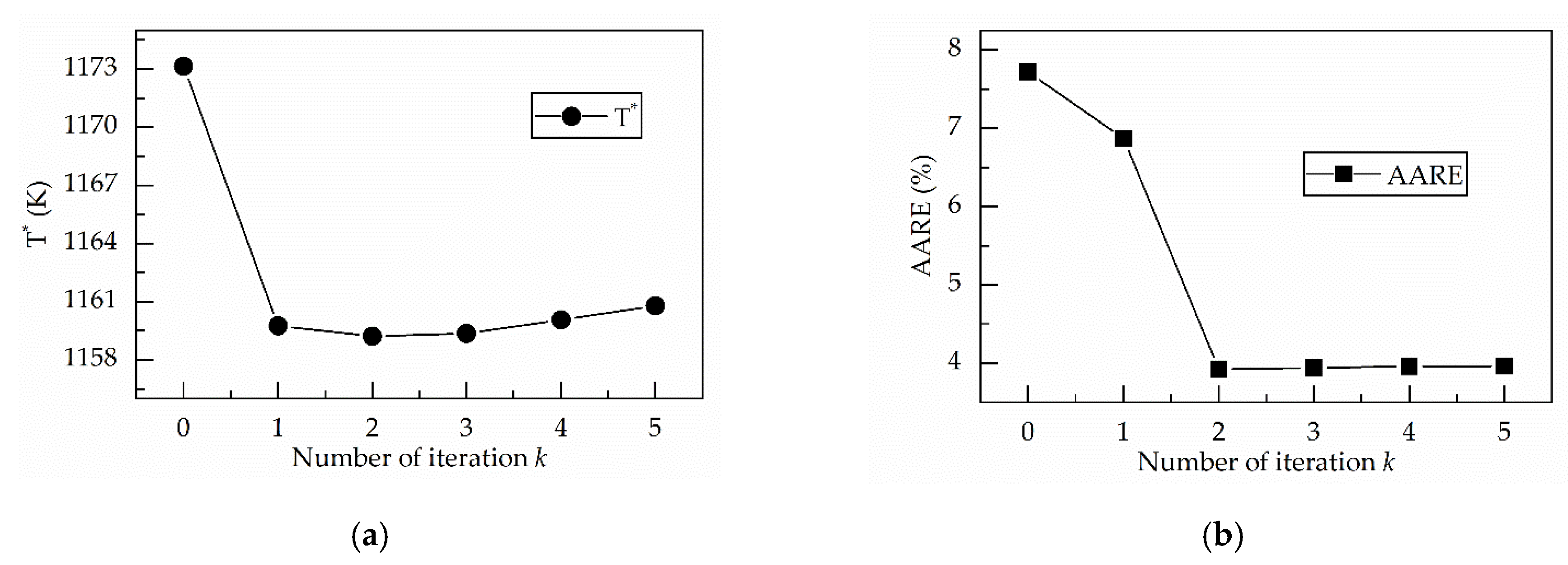
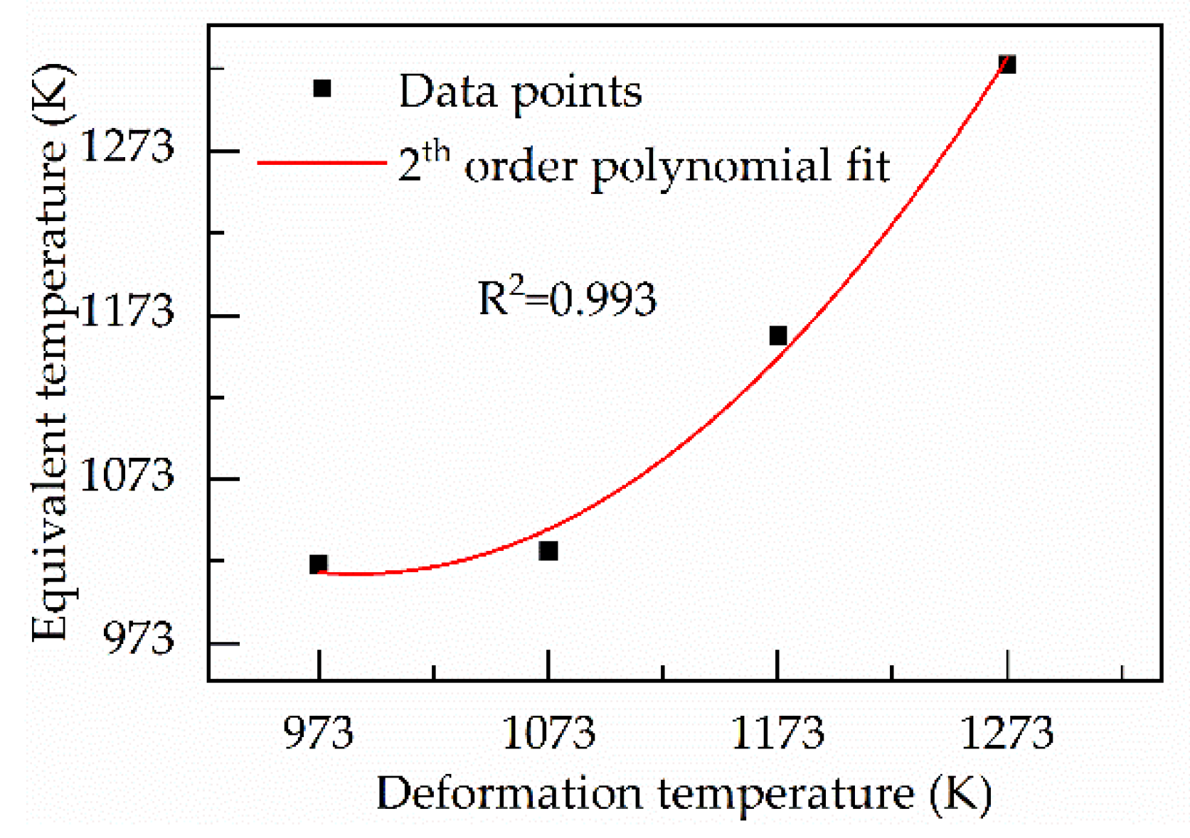
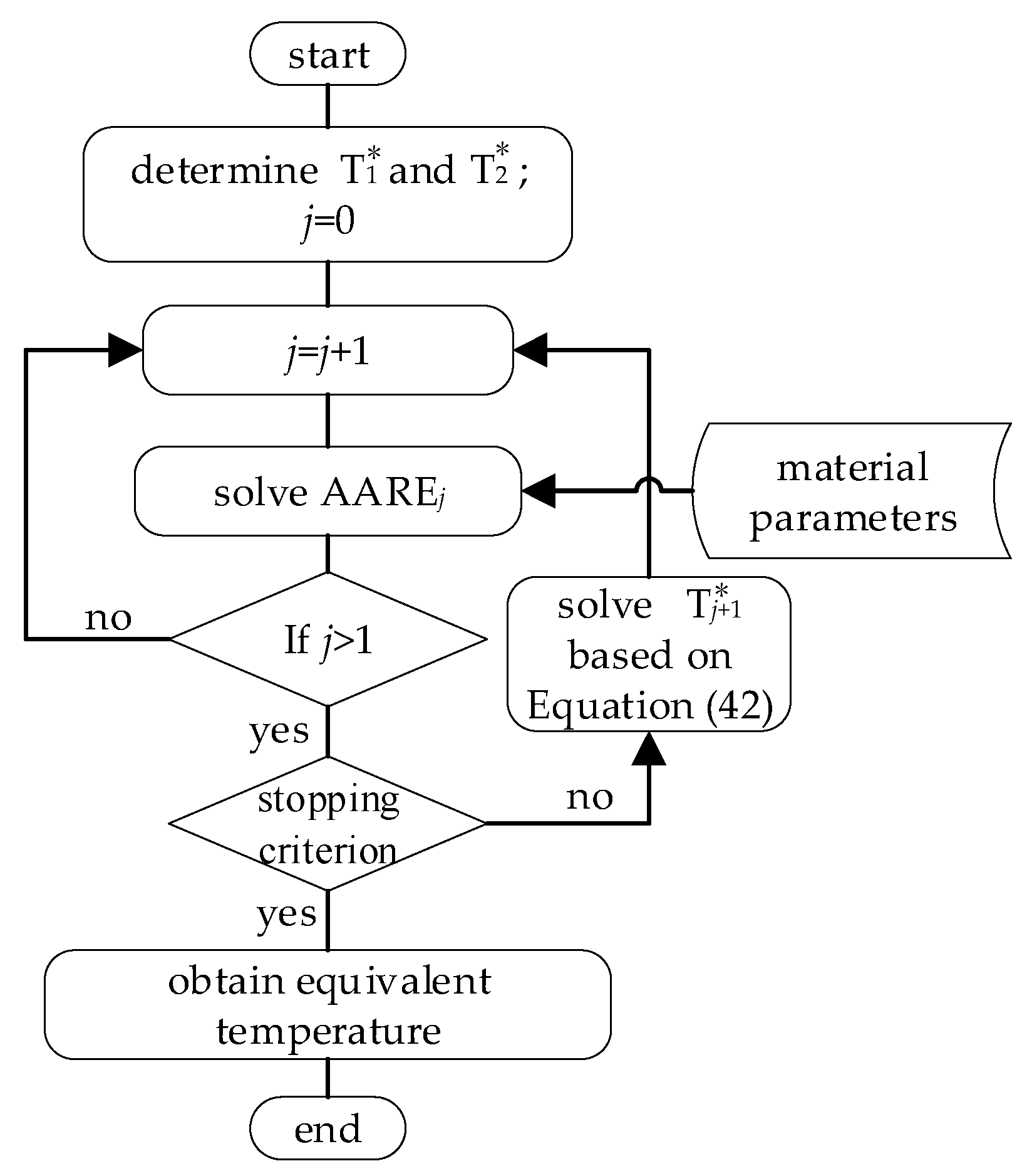
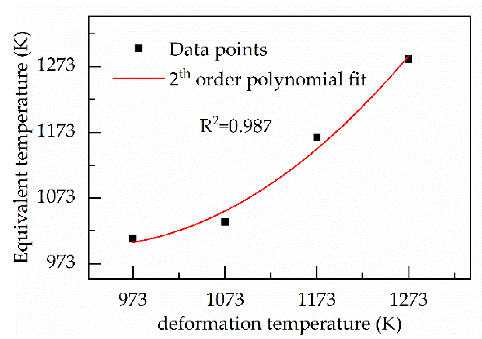
4.2.2. Solving the Equivalent Temperature

After it is determined the material constants under different strains, a line search method is still used to determine the equivalent temperature T*. Therefore, it is established the relationship between the equivalent temperature T* and AARE, which is shown in Equation (31).

$$g({\mathrm{T}}^{*})=\mathrm{AARE}$$

(31)

A line search method can be used to obtain the minimum value of AARE. Thus, Equation (32) is established.

$${\mathrm{T}}_{i+1}^{*}={\mathrm{T}}_j^{*}-{\gamma }_A^T{k}_j^T$$

(32)

Where the positive scalar ${\gamma }_A^T$ is called the step length. The success of a line search method depends on effective choices of both the direction $k_j^T$ and the step length ${\gamma }_A^T$. Moreover, ${\gamma }_A^T$ = 2 holds.

The value of material constants changes with the value of strain. Therefore, it is complicated about a functioning relationship between T* and AARE. Similarly, A search direction $k_j^T$ can be computed based on the secant method.

$$k_j^T=\frac{{\mathrm{AARE}}_j-{\mathrm{AARE}}_{j-1}}{{\mathrm{T}}_j^{*}-{\mathrm{T}}_{j-1}^{*}}(i\ge 2)$$

(33)

To converge faster, if the AARE_j−1-value is greater than the AARE_j-value, ${\mathrm{T}}_{j-1}^{*}$ is used as ${\mathrm{T}}_j^{*}$ in Equation (33). Thus, Equation (34) is obtained.

$${\mathrm{T}}_{j+1}^{*}=\{\begin{array}{ll}{\mathrm{T}}_j^{*}-{\gamma }_A^T\frac{{\mathrm{AARE}}_j-{\mathrm{AARE}}_{j-1}}{{\mathrm{T}}_j^{*}-{\mathrm{T}}_{j-1}^{*}}& ({\mathrm{AARE}}_j\le {\mathrm{AARE}}_{j-1})\\ 0.5\left({\mathrm{T}}_j^{*}+{\mathrm{T}}_{j-1}^{*}\right)& ({\mathrm{AARE}}_j={\mathrm{AARE}}_{j-1})(j>2)\\ {\mathrm{T}}_{j-1}^{*}-{\gamma }_A^T\frac{{\mathrm{AARE}}_j-{\mathrm{AARE}}_{j-1}}{{\mathrm{T}}_j^{*}-{\mathrm{T}}_{j-1}^{*}}& ({\mathrm{AARE}}_j>{\mathrm{AARE}}_{j-1})\end{array}$$

(34)

Similarly, there is not an equation about obtaining the values of ${\mathrm{T}}_1^{*}$ and ${\mathrm{T}}_2^{*}$ in Equation (34). Therefore, other methods are used to determine the values of ${\mathrm{T}}_1^{*}$ and ${\mathrm{T}}_2^{*}$. The deformation temperature can be used as ${\mathrm{T}}_1^{*}$. Moreover, the method of determining ${\mathrm{T}}_2^{*}$ is as follows:

Rearranging Equation (19):

$$\mathrm{T}=-\frac{{10}^3\times \mathrm{Q}}{\mathrm{R}\ln (\dot{\epsilon }/\{\mathrm{A}\left[\sinh \right(\alpha \sigma {\left)\right]}^n\})}$$

(35)

After obtaining material constants, a corresponding T-value is determined by substituting $\dot{\epsilon }$-value and σ-value in Equation (35). Because experimental and predicted values of stress are not equal, the deformation temperature value is not equal to T-value obtained from Equation (35). At a certain deformation temperature, there are 13 different strain (0.10, 0.15, 0.20, 0.25, 0.30, 0.35, 0.40, 0.45, 0.50, 0.55, 0.60, 0.65 and 0.70) and 4 different strain rates (0.001, 0.01, 0.1 and 1 s⁻¹) selected. Therefore, there are 52 experimental data points at a certain deformation temperature. Moreover, 52 values of T are determined by substituting $\dot{\epsilon }$-value and σ-value of the 52 experimental data points in Equation (35). Moreover, the mean value of the set of T-value can be used as ${\mathrm{T}}_2^{*}$.

After determining ${\mathrm{T}}_1^{*}$ and ${\mathrm{T}}_2^{*}$, the equivalent temperature ${\mathrm{T}}_{j+1}^{*}$ can be calculated based on Equation (34). However, a stopping criterion is still needed to terminate the iterative process. The error of AARE-value from the current iteration to the previous one is used as the stopping criterion, which is shown in Equation (36).

$${\mathrm{AARE}}_j-{\mathrm{AARE}}_{j-1}<{10}^{-3}$$

(36)

In Equation (31), AARE_i is determined based on 52 different experimental data points, thus N = 52 in Equation (24). When Equation (36) is met, the corresponding equivalent temperature is determined under a specific temperature. Under different deformation temperatures, the corresponding equivalent temperatures can be calculated by repeating the above process, which is shown in Figure 9.

4.2.3. Optimizing the Material Parameters and Equivalent Temperatures

In Section 4.2.1 and Section 4.2.2, it is determined the approximation of the material constants and the equivalent temperature, respectively. However, in Section 4.2.1, the deformation temperatures are used instead of the equivalent temperature while solving the material constants. Namely, the process of solving the material constants is independent of the equivalent temperature. In Section 4.2.2, determining equivalent temperatures is dependent on the above material constants. Therefore, a group of new material constants is obtained based on the equivalent temperature. Similarly, the new equivalent temperatures are determined based on the new material constants. Based on the above analysis, a new iterative process is proposed to improve the prediction accuracy by optimizing the material constants and the equivalent temperature, which is shown in Figure 10.

The iterative method is used to optimize the prediction accuracy, so a stopping criterion is necessary. Equation (36) is still used as the stopping criterion for this optimization process. However, there are 13 different strain, 4 different strain rates and 4 different deformation temperatures selected. Namely, there are 208 different data points used to determine AARE. Thus, N is 208 in Equation (24).

Based on Figure 10, the solution process of solving the material constants under different strain is independent of each other. The strain of 0.30 is still taken as an example, which is used to show the change in related variables during the process of optimizing the material constants, as shown in Figure 11. Meanwhile, when k = 0, the ordinates of the corresponding data point in Figure 11a,b are the initial guess of α = 0.01162 MPa⁻¹ and the corresponding R², respectively.

Similarly, based on Figure 10, the solution process of solving the equivalent temperatures under different deformation temperatures is independent of each other. The deformation temperature of 1173.15 K is taken as an example, which is used to show the change in related variables during the process of optimizing the deformation temperature, as shown in Figure 12. Moreover, when k = 0, the ordinates of the corresponding data point in Figure 12a,b are the initial guess of T* = 1173.15 K and the corresponding AARE, respectively.

$${\mathrm{T}}^{*}=d_0+d_1\mathrm{T}+d_2{\mathrm{T}}^2$$

(37)

$$\{\begin{array}{l}\sigma =\frac{1}{\alpha }\ln \left\{{\left(\frac{Z}{A}\right)}^{1/n}+{\left[{\left(\frac{Z}{A}\right)}^{2/n}+1\right]}^{1/2}\right\}\\ Z=\dot{\epsilon }\exp \{\mathrm{Q}/[R(d_0+d_1\mathrm{T}+d_2{\mathrm{T}}^2)]\}\end{array}$$

(38)

Through the above optimization process, it is obtained the final values of material constants and equivalent temperatures. The polynomial is still used to describe the relationship between material constants and strains. By adjusting the order of the polynomial, it is found that the fifth-order polynomial is used to obtain a very good correlation and generalization, which is shown in Equation (18) and Figure 13. Similarly, the second-order polynomial is selected to describe the relationship between the deformation temperatures and the equivalent temperatures by adjusting the order of the polynomial, which is shown in Equation (38) and Figure 14. The coefficients of the relevant polynomial is shown in

Table 3. Coefficients of the polynomial for α, n, Q and lnA in the msA-type equation.

α (MPa−1)	n	Q (kJ·mol−1)	lnA	T* (K)
α0 = 0.0099	N0 = 8.1874	Q0 = 441.1503	A0 = 42.0394	d0 = 4839.6758
α1 = −0.0159	N1 = −26.3749	Q1 = −2274.7592	A1 = −239.5653	d1 = −7.7319
α2 = 0.0330	N2 = 97.1817	Q2 = 8516.0320	A2 = 915.6306	d2 = 0.0039
α3 = −0.0012	N3 = −199.2349	Q3 = −16,792.012	A3 = −1834.8319
α4 = −0.0638	N4 = 214.8862	Q4 = 16,706.7723	A4 = 1847.7995
α5 = 0.0463	N5 = −92.8376	Q5 = −6637.2152	A5 = −740.3887

. Concerning the msA-type equation, the predicted stress can be obtained based on Equation (39), which is obtained by substituting Equation (38) in Equation (39). Figure 15 is shown the predicted stress from the modified strain-compensated Arrhenius-type (msA-type) equation.

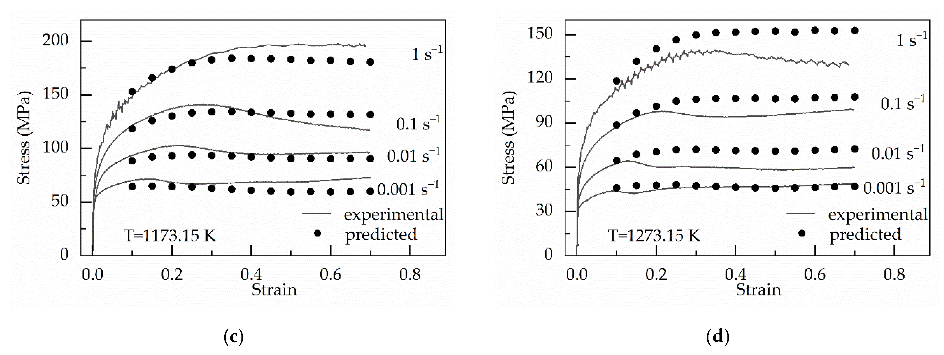
4.3. Establishing the Original Hensel–Spittel (oHS) Equation

Taking the logarithms on both sides of Equation (9) gives:

$$\ln [\sinh (\alpha \sigma )]=\ln (\mathrm{A})+m_1\mathrm{T}+m_2\ln (\epsilon )+m_3\ln (\dot{\epsilon })+m_4/\epsilon +m_5\mathrm{T}\ln (1+\epsilon )+m_6\epsilon$$

(39)

Based on Equation (10), the other material parameters are obtained by the multiple regression analysis, as listed in

Table 4. Material parameters in the oHS equation.

A	m1	m2	m3	m4	m5	m6
147.9874	−0.0044	−0.4507	0.1901	−0.0313	0.0024	−1.0751

. Figure 16 shows the predicted stress from the oHS constitutive equation.

4.4. Establishing the Modified Hensel–Spittel Constitutive Equation

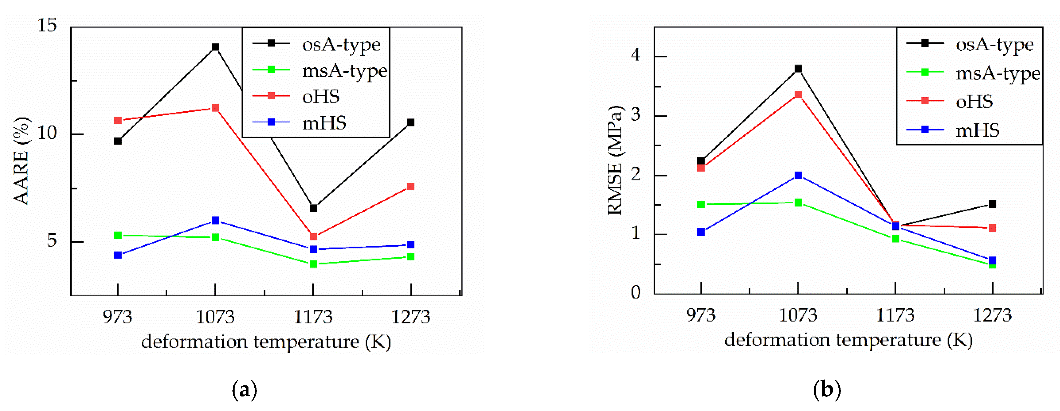
Regarding the modified Hensel–Spittel constitutive equation, taking the logarithms on both sides of Equation (10) gives:

$$\ln [\sinh (\alpha \sigma )]=\ln (\mathrm{A})+m_1{\mathrm{T}}^{*}+m_2\ln (\epsilon )+m_3\ln (\dot{\epsilon })+m_4/\epsilon +m_5{\mathrm{T}}^{*}\ln (1+\epsilon )+m_6\epsilon$$

(40)

About Equation (40), it is assumed that T* is determined. When the material parameter α is obtained, the other material parameters A, m₁, m₂, m₃, m₄, m₅ and m₆, can be solved by multiple regression analysis. When the value of α changes, it will be obtained the different values of the material parameters A, m₁, m₂, m₃, m₄, m₅ and m₆ and the prediction accuracy of the constitutive equation will also change. Therefore, the reasonable value of α can be obtained by a line search method. Moreover, the deformation temperatures can be used instead of the equivalent temperatures in the processes of solving the material parameters.

The values of R² and AARE can be used to measure the prediction accuracy of constitutive equations. Therefore, the values of AARE can be used to determine the material parameters and the equivalent temperature in the modified Hensel–Spittel equation.

Substituting T* = T in Equation (40) yields:

$$\ln [\sinh (\alpha \sigma )]=\ln (\mathrm{A})+m_1\mathrm{T}+m_2\ln (\epsilon )+m_3\ln (\dot{\epsilon })+m_4/\epsilon +m_5\mathrm{T}\ln (1+\epsilon )+m_6\epsilon$$

(41)

Based on a linear search, Equation (31) and Equation (34) is established:

$$h(\alpha )=\mathrm{AARE}$$

(42)

$${\alpha }_{i+1}=\{\begin{array}{ll}{\alpha }_i-{\gamma }_{HS}^{\alpha }\frac{{\mathrm{AARE}}_i-{\mathrm{AARE}}_{i-1}}{{\alpha }_i-{\alpha }_{i-1}}& ({\mathrm{AARE}}_i<{\mathrm{AARE}}_{i-1})\\ 0.5\left({\alpha }_i+{\alpha }_{i-1}\right)& ({\mathrm{AARE}}_i={\mathrm{AARE}}_{i-1})(i>2)\\ {\alpha }_{i-1}-{\gamma }_{HS}^{\alpha }\frac{{\mathrm{AARE}}_i-{\mathrm{AARE}}_{i-1}}{{\alpha }_i-{\alpha }_{i-1}}& ({\mathrm{AARE}}_i>{\mathrm{AARE}}_{i-1})\end{array}$$

(43)

where the positive scalar ${\gamma }_{HS}^{\alpha }$ is the step length and ${\gamma }_{HS}^{\alpha }$ = 10⁻⁸ holds. The values of α₁ and α₂ are the values of α under the strain of 0.10 and 0.70, which are obtained based on the original strain-compensated Arrhenius-type equation. Equation (43) can be used to update the values of α_i+1 in the iterative process. A linear search can be performed based on Figure 17 and it is finally determined the more reasonable approximations of the material parameters α, A, m₁, m₂, m₃, m₄, m₅ and m₆.

When the material parameters are determined, the approximations of T* can be obtained by a line search method. Therefore, Equations (44) and (45) are developed:

$$q({\mathrm{T}}^{*})=\mathrm{AARE}$$

(44)

$${\mathrm{T}}_{i+1}^{*}=\{\begin{array}{ll}{\mathrm{T}}_i^{*}-{\gamma }_{HS}^T\frac{{\mathrm{AARE}}_i-{\mathrm{AARE}}_{i-1}}{{\mathrm{T}}_i^{*}-{\mathrm{T}}_{i-1}^{*}}& ({\mathrm{AARE}}_i\le {\mathrm{AARE}}_{i-1})\\ 0.5\left({\mathrm{T}}_i^{*}+{\mathrm{T}}_{i-1}^{*}\right)& ({\mathrm{AARE}}_i{=\mathrm{AARE}}_{i-1})(i>2)\\ {\mathrm{T}}_{i-1}^{*}-{\gamma }_{HS}^T\frac{{\mathrm{AARE}}_i-{\mathrm{AARE}}_{i-1}}{{\mathrm{T}}_i^{*}-{\mathrm{T}}_{i-1}^{*}}& ({\mathrm{AARE}}_i>{\mathrm{AARE}}_{i-1})\end{array}$$

(45)

where the positive scalar ${\gamma }_{HS}^T$ is called the step length and ${\gamma }_{HS}^T$ = 0.3 holds. By solving AARE in Equation (45), N in Equation (24) is 208.

Equation (45) can be used to update the values of ${\mathrm{T}}_{HS}^{*}$ in the iterative process. However, the values of ${\mathrm{T}}_1^{*}$ and ${\mathrm{T}}_2^{*}$ still needs to be determined. The corresponding equivalent temperatures need to be solved based on the experimental data under different temperatures. Therefore, the value of a specific deformation temperature can be used as ${\mathrm{T}}_1^{*}$ to solve the corresponding equivalent temperature.

Rearranging Equation (41) gives:

$$\mathrm{T}=\frac{\ln [\sinh (\alpha \sigma )]-[\ln (\mathrm{A})+m_2\ln (\epsilon )+m_3\ln (\dot{\epsilon })+m_4/\epsilon +m_6\epsilon ]}{m_1+m_5\ln (1+\epsilon )}$$

(46)

At a specific deformation temperature, there are 52 different experimental data points under different deformation conditions, including 13 different strain and 4 different strain rates selected. Therefore, when the corresponding experimental data are substituted in Equation (46), 52 different values of T are determined. The mean of the set of T-value can be used as the value of ${\mathrm{T}}_2^{*}$.

A linear search can be performed to find out a more reasonable approximation of T*, which is shown in Figure 18. Under various deformation temperatures, the corresponding equivalent temperatures can be solved by repeating the above process, which is shown in Figure 18.

Based on Section 4.2.3, a similar optimization process can be applied. The more reasonable values of the material parameters and the equivalent temperatures are obtained; the results are shown in

Table 5. The material parameters in the mHS equation.

α (MPa−1)	A	m1	m2	m3	m4	m5	m6
0.0062	99.0968	−0.0041	−0.3653	0.1716	−0.0502	0.0019	−1.0019

and Figure 19. The second-order polynomial is used to describe the behavior between the deformation temperatures and the equivalent temperatures, which is shown in Equation (37). The coefficients of the polynomial are shown in

Table 6. Coefficients of the polynomial for the equivalent temperatures in the mHS equation.

d0	d1	d2
2999.7217	−4.3393	0.0024

. Equation (47) shows the modified Hensel–Spittel constitutive equation, which is established by substituting Equation (37) in Equation (10). Figure 20 shows the predicted stress obtained from the modified Hensel–Spittel (mHS) equation.

$$\sinh (\alpha \sigma )=\mathrm{A}\exp [m_1(d_0+d_1\mathrm{T}+d_2{\mathrm{T}}^2)]{\epsilon }^{m_2}{\dot{\epsilon }}^{m_3}\exp (m_4/\epsilon ){(1+\epsilon )}^{m_5(d_0+d_1\mathrm{T}+d_2{\mathrm{T}}^2)}\exp (m_6\epsilon )$$

(47)

5. Discussion

Based on the above results, it is obtained the predicted stress from the original strain-compensated Arrhenius-type (osA-type) equation, the modified strain-compensated Arrhenius-type (msA-t) equation, the original Hensel–Spittel (oHS) equation and the modified Hensel–Spittel (mHS) equation. A comparative study is made to determine which constitutive equation is more suitable for the alloy. Therefore, some measure methods in statistics are needed to compare the prediction accuracy of the constitutive equations, including R², AARE, the relative errors (RE) and the average root mean square error (RMSE).

Regarding R², it is used to verify the prediction accuracy of the constitutive equation, based on measuring how strong a linear relationship between the experimental and predictive stress is. The higher value of R² means the constitutive equation has a higher prediction accuracy. The value of R² of the msA-type equation is the biggest at 0.981, which is followed by the mHS equation (0.978), the oHS equation (0.938). The R²-value of the osA-type equation is the smallest, at 0.925.

Figure 21 shows the relationship between the experimental stress and the predicted stress from the four constitutive equations. Meanwhile, one straight line σ_p = σ_e is introduced into Figure 21. When the predicted stress is equal to the experimental stress, the corresponding data point is located on the straight line σ_p = σ_e.

In Figure 21, there is a different distance from different points to the straight line, which suggests that there is a different error between the experimental and predictive stress for different data points.

In statistics, normalization can adjust the error of different data points to a notionally common scale, namely, the same comparison standard for every predicted stress value. Therefore, as a normalized unbiased statistical parameter, the average absolute relative error (AARE) is always used to verify the predictability of the constitutive equation. The smaller value of AARE suggests that the predictability of the constitutive equation is stronger.

Regarding the AARE, the msA-type model has a minimum (4.70%), when compared to the mHS equation (4.98%), the osA-type equation (10.23%) and the oHS equation (8.46%).

Moreover, the relative errors (RE) is generally applied to show the error distribution of the constitutive equation. The relative errors (RE)are calculated via a term-by-term comparison of predicted and experimental values, which is shown in Equation (48).

$$\mathrm{RE}=\frac{(E_i-P_i)}{E_i}\times 100\%$$

(48)

where E_i and P_i still are the experimental and predicted values, respectively.

Figure 22 shows the distribution of relative error values of the four constitutive equations. It can be obtained that the relative errors obtained from the osA-type equation and the oHS equation vary from −27.7% to 22.1% and −25.1% to 22.2%, respectively. In contrast, the relative error of the msA-type equation and the mHS equation ranges from −14.5% to 16.6% and −11.9% to 20.1%, respectively.

Moreover, in the RE-values range from −10% to 10%, there are 97.83% and 84.13% of the numbers of relative errors of the modified strain-compensated Arrhenius-type (ms–cA-type) equation and the modified Hensel–Spittel (mHS) equation. Compared with the two modified constitutive equation, 57.21% and 67.31% of the RE-number of the original strain-compensated Arrhenius-type (os–cA-type) equation and the original Hensel–Spittel (oHS) equation locate between RE-values of −10% and 10%.

In addition, the average root mean square error (RMSE) is a statistical measures, which is used to evaluate the performance of the four constitutive equation further [15,52]. The expression of RMSE is as follows:

$$\mathrm{RMSE}=\sqrt{\frac{1}{N}{\displaystyle \sum _{i=1}^N{(E_i-P_i)}^2}}$$

(49)

where RMSE is the average root mean square error, E_i is the experimental data, P_i is the predicted value obtained from the model, and N is the total number of data employed in the investigation (N = 208). The smaller the value of RMSE, the higher the prediction accuracy of the constitutive equation. The RMSE-value of the msA-type equation (0.60) is the smallest. Moreover, the RMSE-value of the mHS, msA-type and oHS equation is 0.65, 1.07 and 1.20 MPa, respectively.

AARE and RMSE can be used to explain that the prediction accuracy of the constitutive equation changes as the rise of deformation temperatures. Figure 23 shows the AARE-values and RMSE-values obtained based on the experimental and predicted stress under different deformation temperatures.

In Figure 23b, in the beginning, the RMSE-values of the four constitutive equations increase with increasing the deformation temperature. Because the increase of the flow stress is relatively smaller, which is shown in Figure 2, the AARE-values of the four constitutive equations also increase as the deformation temperature rises. Moreover, regarding the four constitutive equations, the AARE-value of every constitutive equation reaches its maximum when the deformation temperature is 1073.15 K. Although there is a similar trend about the RMSE-values and AARE-values of the four constitutive equations, every modified constitutive equation (namely, the msA-type and mHS equations) has a smaller RMSE-value and AARE-value when compared to any original constitutive equation (namely, the osA-type and oHS equations).

As the deformation temperature rises from 1073.15 to 1173.15 K, the AARE-values of the original constitutive equation decrease sharply because the reduced ratio of the RMSE-value of the original constitutive equation is higher than that of the flow stress. When the deformation temperature reaches 1173.15 K, the AARE of every original constitutive equations takes its minimum, which is higher than the AARE of any modified constitutive equations at 1173.15 K.

With increasing the deformation temperatures from 1173.15 to 1273.15 K, the AARE-values of the original constitutive equations increases sharply. The reason is that, while there is a relatively small change in the RMSE of the original constitutive equations in Figure 23b, the flow stress relatively significantly reduces, for example, data in Figure 2.

Regarding the two modified constitutive equations, in Figure 23b, the RMSE-value of every constitutive equation keeps decreasing with increasing the deformation temperature from 1073.15 to 1273.15 K, while the flow stress also keeps reducing. Therefore, the change in the AARE-value of the two constitutive equations is relatively small in the deformation temperature range from 1073.15 to 1273.15 K.

Under the different deformation temperature, every modified constitutive equation has a smaller AARE-value than any original constitutive equation. Based on the above analysis, the two modified constitutive equation can give a more reasonable description of the relationship between the flow stress and deformation temperatures.

Table 7. R², AARE, RMSE and relative errors (RE) of the original strain-compensated Arrhenius-type (osA-type) equation, the modified strain-compensated Arrhenius-type (msA-type) equation, the original Hensel–Spittel (oHS) equation and the modified Hensel–Spittel (mHS) equation.

Constitutive Equation	R2	AARE (%)	RMSE (MPa)	Max of RE (%)	Min of RE (%)	Mean of RE (%)
osA-type	0.925	10.23	1.20	22.15	−27.74	0.17
oHS	0.938	8.46	1.07	22.23	−25.08	−0.83
mHS	0.978	4.98	0.65	−11.87	−20.08	0.44
msA-type	0.981	4.70	0.60	−14.52	16.64	−0.11

shows the R², AARE, RE and RMSE obtained based on the different constitutive equations. In summary, it is easily found that the two modified constitutive equations (namely, the msA-type and mHS equations) give more accurate results than the two original constitutive equations (namely, the osA-type and oHS equations).

6. Conclusions

In the present study, the warm and hot deformation behavior of 20Cr2Ni4A alloy steel is described based on the compression tests in temperatures ranging from 973.15 to 1273.15 K and strain rates of 0.001–1 s⁻¹. The four constitutive equations can be used to predict the flow stress, including the original strain-compensated Arrhenius-type (osA-type) equation, the original Hensel–Spittel (oHS) equation, the modified strain-compensated Arrhenius-type (msA-type) equation and the modified Hensel–Spittel (mHS) equation. The msA-type equation and the mHS equation are developed by revising the deformation temperatures in the osA-type equation and oHS equation, respectively. Several conclusions are obtained by comparing the predicted stress from four equations with the experimental, which are shown below.

(1)

The new method is proposed by combining multiple linear regression with the iterative method, which can determine the parameters in the msA-type equation and the mHS equation. Moreover, the new method can optimize the parameters to improve the predication accuracy of the two modified constitutive equations;

(2)

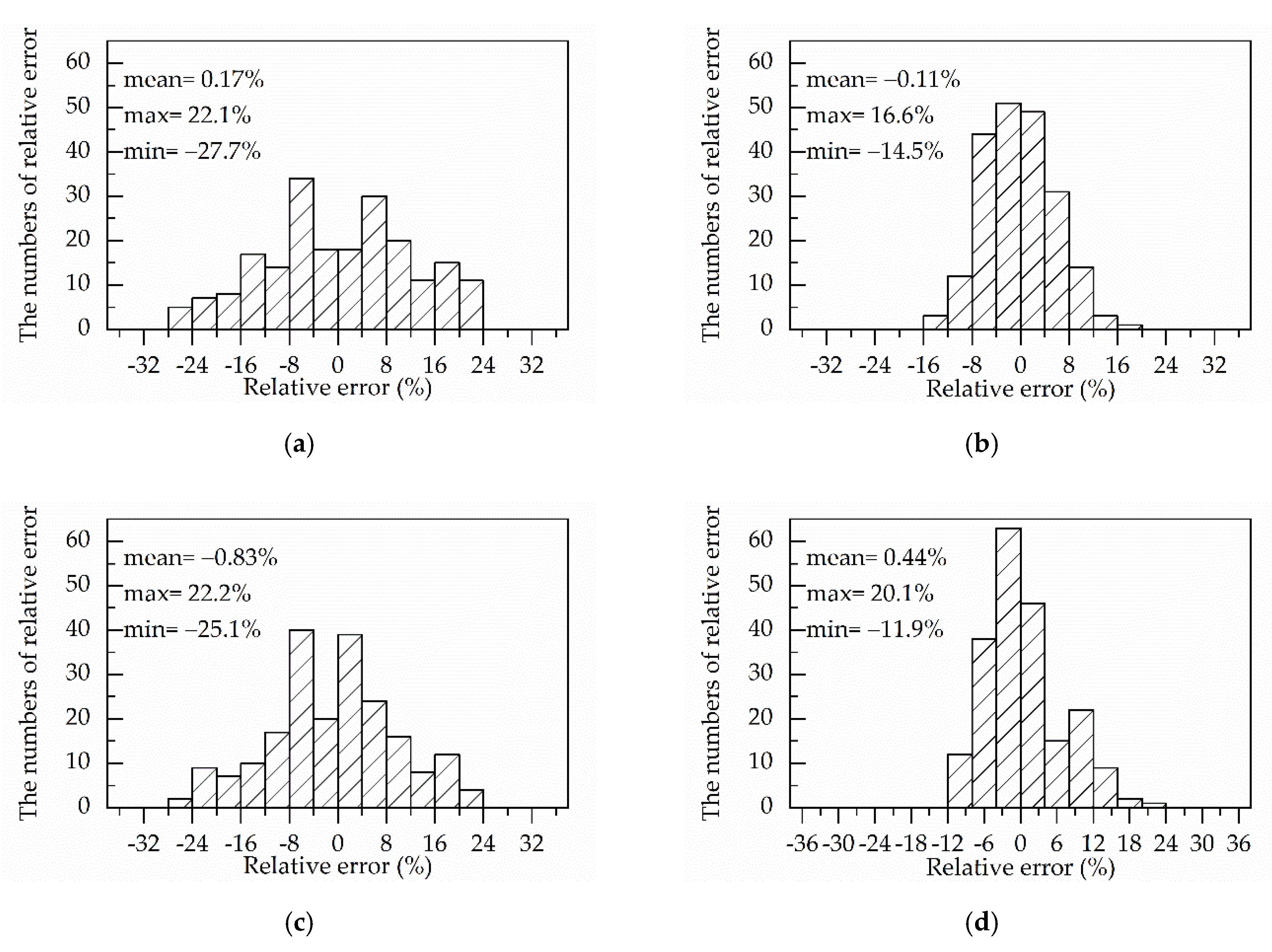
The two original constitutive equations (namely, the osA-type and oHS equation) had a relatively lower prediction accuracy, with R-value, AARE-value and RMSE-value of 0.925, 10.23% and 1.20 MPa for the original strain-compensated Arrhenius-type (osA-type) equation and of 0.938, 8.46% and 1.07 MPa for the original Hensel–Spittel (oHS) equation;

(3)

The prediction accuracy of the modified strain-compensated Arrhenius-type (msA-type) equation is the highest because the msA-type equation has the highest R-value (0.981), the lowest AARE-value (4.70%) and MRSE-value (0.6 MPa). Moreover, the R-value, AARE-value and RMSE-value of the modified Hensel–Spittel (mHS) equation are 0.978, 4.98% and 0.65 MPa, respectively. Therefore, the two modified have similar prediction accuracy and every modified constitutive equation (namely, the msA-type and mHS equation) has higher prediction accuracy than any original constitutive equation (namely, the osA-type and oHS equation);

(4)

Regarding the above two modified constitutive equations, there is a smaller difference between AARE under different deformation temperatures and every AARE-valve is relatively small.

In contrast, for the two original constitutive equations, the changes in AARE-values are evident as the rise of the deformation temperature and the AARE-value under different deformation temperatures is higher. The result suggests that the two modified constitutive equations can be more accurate in describing the relationship between the deformation temperature and the flow stress.

References

1. Tokita, Y.; Nakagaito, T.; Tamai, Y.; Urabe, T. Stretch formability of high strength steel sheets in warm forming. J. Mater. Process. Technol. 2017, 246, 77–84. [Google Scholar] [CrossRef]
2. Chino, Y.; Nakaura, Y.; Ohori, K.; Kamiya, A.; Mabuchi, M. Mechanical properties at elevated temperature of a hot-deformed Mg–Al–Ca–Mn–Sr alloy. Mater. Sci. Eng. A 2007, 452, 31–36. [Google Scholar] [CrossRef]
3. Li, Y.Y.; Zhao, S.D.; Fan, S.Q.; Zhong, B. Plastic properties and constitutive equations of 42CrMo steel during warm forming process. Mater. Sci. Technol. 2014, 30, 645–652. [Google Scholar] [CrossRef]
4. Fujikawa, S.; Yoshioka, H.; Shimamura, S. Cold- and warm-forging applications in the automotive industry. J. Mater. Process. Technol. 1992, 35, 317–342. [Google Scholar] [CrossRef]
5. Niechajowicz, A.; Tobota, A. Warm deformation of carbon steel. J. Mater. Process. Technol. 2000, 106, 123–130. [Google Scholar] [CrossRef]
6. Lin, Y.C.; Chen, M.S. Study of microstructural evolution during static recrystallization in a low alloy steel. J. Mater. Sci. 2009, 44, 835–842. [Google Scholar] [CrossRef]
7. Lin, Y.C.; Chen, M.S.; Zhong, J. Study of static recrystallization kinetics in a low alloy steel. Comput. Mater. Sci. 2008, 44, 316–321. [Google Scholar] [CrossRef]
8. Ben, N.-Y.; Zhang, D.-W.; Liu, N.; Zhao, X.-P.; Guo, Z.-J.; Zhang, Q.; Zhao, S.-D. FE modeling of warm flanging process of large T-pipe from thick-wall cylinder. Int. J. Adv. Manuf. Technol. 2017, 93, 3189–3201. [Google Scholar] [CrossRef]
9. Shin, H.; Kim, J.B. A phenomenological constitutive equation to describe various flow stress behaviors of materials in wide strain rate and temperature regimes. J. Eng. Mater. 2010, 132, 021009. [Google Scholar] [CrossRef]
10. Lin, Y.C.; Liu, G. A new mathematical model for predicting flow stress of typical high-strength alloy steel at elevated high temperature. Comput. Mater. Sci. 2010, 8, 48–54. [Google Scholar] [CrossRef]
11. Lin, Y.C.; Chen, X.M. A critical review of experimental results and constitutive descriptions for metals and alloys in hot working. Mater. Des. 2011, 32, 1733–1759. [Google Scholar] [CrossRef]
12. Abbasi-Bani, A.; Zarei-Hanzaki, A.; Pishbin, M.H.; Haghdadi, N. A comparative study on the capability of Johnson-Cook and Arrhenius-type constitutive equations to describe the flow behavior of Mg-6A1-1Zn alloy. Mech. Mater. 2014, 71, 52–61. [Google Scholar] [CrossRef]
13. Wen, T.; Liu, L.T.; Huang, Q.; Chen, X.; Fang, J.Z. Evaluation on prediction abilities of constitutive models considering FEA application. J. Cent. South Univ. 2018, 25, 1251–1262. [Google Scholar] [CrossRef]
14. Xia, Y.N.; Zhang, C.; Zhang, L.W.; Shen, W.F.; Xu, Q.H. A comparative study of constitutive models for flow stress behavior of medium carbon Cr–Ni–Mo alloyed steel at elevated temperature. J. Mater. Res. 2017, 32, 3875–3884. [Google Scholar] [CrossRef]
15. Ma, Z.W.; Hu, F.Y.; Wang, Z.J.; Fu, K.J.; Wei, Z.X.; Wang, J.J.; Li, W.J. Constitutive Equation and Hot Processing Map of Mg-16Al Magnesium Alloy Bars. Materials 2020, 13, 3107. [Google Scholar] [CrossRef] [PubMed]
16. He, A.; Xie, G.L.; Zhang, H.L.; Wang, X.T. A comparative study on Johnson-Cook, modified Johnson-Cook and Arrhenius-type constitutive models to predict the high temperature flow stress in 20CrMo alloy steel. Mater. Des. 2013, 52, 677–685. [Google Scholar] [CrossRef]
17. Li, Y.; Ji, H.; Cai, Z.; Tang, X.; Li, Y.; Liu, J. Comparative study on constitutive models for 21-4N heat resistant steel during high temperature deformation. Materials 2019, 12, 1893. [Google Scholar] [CrossRef] [Green Version]
18. Li, H.Y.; Wang, X.F.; Wei, D.D.; Hu, J.D.; Li, Y.H. A comparative study on modified Zerilli-Armstrong, Arrhenius-type and artificial neural network models to predict high-temperature deformation behavior in T24 steel. Mater. Sci. Eng. A 2012, 536, 216–222. [Google Scholar] [CrossRef]
19. Samantaray, D.; Mandal, S.; Bhaduri, A.K. A comparative study on Johnson Cook, modified Zerilli–Armstrong and Arrhenius-type constitutive models to predict elevated temperature flow behavior in modified 9Cr–1Mo steel. Comput. Mater. Sci. 2009, 47, 568–576. [Google Scholar] [CrossRef]
20. Li, H.-Y.; Li, Y.-H.; Wang, X.-F.; Liu, J.-J.; Wu, Y. A comparative study on modified Johnson Cook, modified Zerilli–Armstrong and Arrhenius-type constitutive models to predict the hot deformation behavior in 28CrMnMoV steel. Mater. Des. 2013, 49, 493–501. [Google Scholar] [CrossRef]
21. Li, T.; Zhao, B.; Lu, X.; Xu, H.; Zou, D. A Comparative Study on Johnson Cook, Modified Zerilli–Armstrong, and Arrhenius-Type Constitutive Models to Predict Compression Flow Behavior of SnSbCu Alloy. Materials 2019, 12, 1726. [Google Scholar] [CrossRef] [PubMed] [Green Version]
22. Wang, J.; Zhao, G.; Chen, L.; Li, J. A comparative study of several constitutive models for powder metallurgy tungsten at elevated temperature. Mater. Des. 2016, 90, 91–100. [Google Scholar] [CrossRef]
23. Shokry, A.; Gowid, O.D.S.; Kharmanda, G.; Mahdi, E. Constitutive models for the prediction of the hot deformation behavior of the 10%Cr steel alloy. Materials 2019, 12, 2873. [Google Scholar] [CrossRef] [Green Version]
24. Wang, F.; Shen, J.; Zhang, Y.; Ning, Y. A modified constitutive model for the description of the flow behavior of the Ti-10V-2Fe-3Al alloy during hot plastic deformation. Metals 2019, 9, 844. [Google Scholar] [CrossRef] [Green Version]
25. Li, J.; Liu, J. Strain compensation constitutive model and parameter optimization for Nb-contained 316LN. Metals 2019, 9, 212. [Google Scholar] [CrossRef] [Green Version]
26. Hensel, A.; Spittel, T. Kraft-Und Arbeitsbedarf Bildsamer Formgeburgsverfahren: Mit51 Tabellen; Dt Verlag fur Grundstoffindustrie: Wuppertal, Germany, 1978. [Google Scholar]
27. El Mehtedi, M.; Musharavati, F.; Spigarelli, S. Modelling of the flow behaviour of wrought aluminium alloys at elevated temperatures by a new constitutive equation. Mater. Des. 2014, 54, 869–873. [Google Scholar] [CrossRef]
28. Rudnytskyj, A.; Simon, P.; Jech, M.; Gachot, C. Constitutive modelling of the 6061 aluminium alloy under hot rolling conditions and large strain ranges. Mater. Des. 2020, 190, 108568. [Google Scholar] [CrossRef]
29. Wei, G.; Peng, X.; Hadadzadeh, A.; Mahmoodkhani, Y.; Xie, W.; Yang, Y.; Wells, M.A. Constitutive modeling of Mg-9Li-3Al-2Sr-2Y at elevated temperatures. Mech. Mater. 2015, 89, 241–253. [Google Scholar] [CrossRef]
30. Godor, F.; Werner, R.; Lindemann, J.; Clemens, H.; Mayer, S. Characterization of the high temperature deformation behavior of two intermetallic TiAl–Mo alloys. Mater. Sci. Eng. A 2015, 648, 208–216. [Google Scholar] [CrossRef]
31. Rebeyka, C.J.; Button, S.T.; Lajarin, S.F.; Marcondes, P.V.P. Mechanical behavior of HSLA350/440 and DP350/600 steels at different temperatures and strain rates. Mater. Res. Express 2018, 5, 66515. [Google Scholar] [CrossRef]
32. Lin, Y.C.; Wu, Q.; Pang, G.D.; Jiang, X.Y.; He, D.G. Hot tensile deformation mechanism and dynamic softening behavior of Ti–6Al–4V alloy with thick lamellar icrostructures. Adv. Eng. Mater. 2020, 22, 1901193. [Google Scholar] [CrossRef]
33. Pang, L.; Liu, G.C.; Lu, J.P. The experiments for mechanical properties of 20Cr2Ni4 steel and the coefficient definition of constitutive equation. J. Mater. Process. Technol. 2016, 237, 216–234. [Google Scholar] [CrossRef] [Green Version]
34. Wang, W.; Zhao, J.; Zhai, R.X.; Ma, R. Arrhenius-Type Constitutive Model and Dynamic Recrystallization Behavior of 20Cr2Ni4A Alloy Carburizing Steel. Steel Res. Int. 2016, 87, 9999. [Google Scholar] [CrossRef]
35. Springer, P.; Prahl, U. Characterisation of mechanical behavior of 18CrNiMo7-6 steel with and without nb under warm forging conditions through processing maps analysis. J. Mater. Process. Technol. 2016, 237, 216–234. [Google Scholar] [CrossRef]
36. Jin, Y.; Xue, H.; Yang, Z.; Zhang, L.; Zhang, C.; Wang, S.; Luo, J. Constitutive Equation of GH4169 Superalloy and Microstructure Evolution Simulation of Double-Open Multidirectional Forging. Metals 2019, 9, 1146. [Google Scholar] [CrossRef] [Green Version]
37. Sheng, X.; Lei, Q.; Xiao, Z.; Wang, M. Hot Deformation Behavior of a Spray-Deposited Al-8.31Zn-2.07Mg-2.46Cu-0.12Zr Alloy. Metals 2017, 7, 299. [Google Scholar] [CrossRef] [Green Version]
38. Wen, S.; Han, C.; Zhang, B.; Liang, Y.; Ye, F.; Lin, J. Flow Behavior Characteristics and Processing Map of Fe-6.5wt. %Si Alloys during Hot Compression. Metals 2018, 8, 186. [Google Scholar] [CrossRef] [Green Version]
39. Lei, B.; Chen, G.; Liu, K.; Wang, X.; Jiang, X.; Pan, J.; Shi, Q. Constitutive Analysis on High-Temperature Flow Behavior of 3Cr-1Si-1Ni Ultra-High Strength Steel for Modeling of Flow Stress. Metals 2019, 9, 42. [Google Scholar] [CrossRef] [Green Version]
40. Li, Q.; Wang, T.-S.; Li, H.-B.; Gao, Y.-W.; Li, N.; Jing, T.-F. Warm deformation behavior of steels containing carbon of 0. 45% to 1. 26% with marten site starting structure. J. Iron Steel Res. Int. 2010, 17, 34–37. [Google Scholar] [CrossRef]
41. Li, Q.; Wang, T.S.; Jing, T.F.; Gao, Y.W.; Zhou, J.F.; Yu, J.K.; Li, H.B. Warm deformation behavior of quenched medium carbon steel and its effect on microstructure and mechanical properties. Mater. Sci. Eng. A 2009, 515, 38–42. [Google Scholar] [CrossRef]
42. Omale, J.I.; Ohaeri, E.G.; Szpunar, J.A.; Arafin, M.; Fateh, F. Microstructure and texture evolution in warm rolled API 5L X70 pipeline steel for sour service application. Mater. Charact. 2019, 147, 453–463. [Google Scholar] [CrossRef]
43. Huang, Y.C.; Lin, Y.C.; Deng, J.; Liu, G.; Chen, M.S. Hot tensile deformation behaviors and constitutive model of 42CrMo steel. Mater. Des. 2014, 53, 349–356. [Google Scholar] [CrossRef]
44. Cui, M.; Zhao, S.; Chen, C.; Zhang, D.-W.; Li, J.; Li, Y. Study on warm forming effects of the axial-pushed incremental rolling process of spline shaft with 42CrMo steel. Proc. Inst. Mech. Eng. Part E J. Process. Mech. Eng. 2017, 232, 555–565. [Google Scholar] [CrossRef]
45. Momeni, A.; Dehghani, K. Prediction of dynamic recrystallization kinetics and grain size for 410 martensitic stainless steel during hot deformation. Met. Mater. Int. 2010, 16, 843–849. [Google Scholar] [CrossRef]
46. Mirzaee, M.; Keshmiri, H.; Ebrahimi, G.R.; Momeni, A. Dynamic recrystallization and precipitation in low carbon low alloy steel 26NiCrMoV 14–5. Mater. Sci. Eng. A 2012, 551, 25–31. [Google Scholar] [CrossRef]
47. He, Z.B.; Wang, Z.B.; Li, P. A Comparative Study on Arrhenius and Johnson–Cook Constitutive Models for High-Temperature Deformation of Ti2AlNb-Based Alloys. Metals 2019, 9, 123. [Google Scholar] [CrossRef] [Green Version]
48. McQueen, H.J.; Ryan, N.D. Constitutive analysis in hot working. Mater. Sci. Eng. A 2002, 322, 43–63. [Google Scholar] [CrossRef]
49. Slooff, F.A.; Zhou, J.; Duszczyk, J.; Katgerman, L. Constitutive analysis of wrought magnesium alloy Mg–Al4–Zn1. Scripta Metall. 2007, 57, 759–762. [Google Scholar] [CrossRef]
50. Samantaray, D.; Mandal, S.; Bhaduri, A.K. Constitutive analysis to predict high-temperature flow stress in modified 9Cr–1Mo (P91) steel. Mater. Des. 2010, 31, 981–984. [Google Scholar] [CrossRef]
51. Peng, X.; Guo, H.; Shi, Z.; Qin, C.; Zhao, Z. Constitutive equations for high temperature flow stress of TC4-DT alloy incorporating strain, strain rate and temperature. Mater. Des. 2013, 50, 198–206. [Google Scholar] [CrossRef]
52. He, J.; Chen, F.; Wang, B.; Zhu, L.B. A modified Johnson–Cook model for 10% Cr steel at elevated temperatures and a wide range of strain rates. Mater. Sci. Eng. A 2018, 715, 1–9. [Google Scholar] [CrossRef]
Figure 1. Flow chart of the isothermal hot compression.
Metals 10 01169 g001
Figure 2. Flow stress curves of isothermally compressed 20Cr2Ni4A alloy steel at a strain rate of 0.01 s−1.
Metals 10 01169 g002
Figure 3. Relationship between stress and (a) strain rate; (b) deformation temperature under the strain of 0.30.
Metals 10 01169 g003
Figure 4. Relationships between (a) lnσ and ln ε ˙ ; (b) σ and ln ε ˙ ; (c) ln[sinh(ασ)] and ln ε ˙ .
Metals 10 01169 g004
Figure 5. Relationships between (a) 1000/T and In[sinh(ασ)]; (b) In[sinh(αα)] and lnZ.
Metals 10 01169 g005
Figure 6. Relationship between the strain and material constants in the osA-type equation. (a) α; (b) n; (c) Q; (d) A.
Metals 10 01169 g006
Figure 7. Comparison between the experimental and predicted stress by in the original strain-compensated Arrhenius-type (osA)-type equation at temperatures of (a) 973.15 K; (b) 1073.15 K; (c) 1173.15 K; (d) 1273.15 K.
Metals 10 01169 g007aMetals 10 01169 g007b
Figure 8. Process of solving material constants in the modified strain-compensated Arrhenius-type (msA)-type equation by combining multiple regression analysis with a linear search.
Metals 10 01169 g008
Figure 9. Process of solving a single equivalent temperature in the msA-type equation by combining multiple regression analysis with a linear search.
Metals 10 01169 g009
Figure 10. Process of establishing the modified strain-compensated Arrhenius-type (msA-type) equation.
Metals 10 01169 g010
Figure 11. Based on the process in Figure 10, Variation of parameters (a) α; (b) R2 with the numbers of iterations k while optimizing the material constants under strain of 0.30.
Metals 10 01169 g011
Figure 12. Based on the process in Figure 10, the variation of parameters (a) T*; (b) AARE with the numbers of iterations k while optimizing the equivalent temperature under the deformation temperature of 1173.15 K.
Metals 10 01169 g012
Figure 13. Relationship between the strain and material constants in the msA-type equation. (a) α; (b) n; (c) Q; (d) A.
Metals 10 01169 g013
Figure 14. Relationship between the deformation temperatures and the equivalent temperatures in the msA-type equation.
Metals 10 01169 g014
Figure 15. Comparison between the experimental and predicted stress by in the msA-type equation at temperatures of (a) 973.15 K; (b) 1073.15 K; (c) 1173.15 K; (d) 1273.15 K.
Metals 10 01169 g015
Figure 16. Comparison between the experimental and predicted stress by in the original Hensel–Spittel (oHS) equation at temperatures of (a) 973.15 K; (b) 1073.15 K; (c) 1173.15 K; (d) 1273.15 K.
Metals 10 01169 g016aMetals 10 01169 g016b
Figure 17. Process of solving the material parameters in the modified Hensel–Spittel (mHS) equation by combining multiple regression analysis with a linear search.
Metals 10 01169 g017
Figure 18. The process of solving a single equivalent temperature in the mHS equation by combining multiple regression analysis with a linear search.
Metals 10 01169 g018
Figure 19. Relationship between the deformation temperatures and the equivalent temperatures in the mHS equation.
Metals 10 01169 g019
Figure 20. Comparison between the experimental and predicted stress by in the mHS equation at temperatures of (a) 973.15 K; (b) 1073.15 K; (c) 1173.15 K; (d) 1273.15 K.
Metals 10 01169 g020
Figure 21. Correlation between the experimental stress and predicted flow stress values from the (a) osA-type equation; (b) msA-type equation; (c) oHS equation; (d) mHS equation.
Metals 10 01169 g021
Figure 22. Statistical analysis of the relative error from the (a) osA-type equation; (b) msA-type equation; (c) oHS equation; (d) mHS equation.
Metals 10 01169 g022
Figure 23. (a) average absolute relative error (AARE); (b) root mean square error (RMSE) obtained based on the experimental and predicted stress from the four constitutive equations under the different deformation temperatures.
Metals 10 01169 g023