Abstract
Gas tungsten arc welding with an external magnetic field is proven to suppress weld defects while improving welding speed. A three-dimensional numerical model that considers interactions among the arc plasma, weld pool, metal vapor, and external magnetic field is developed. The influences of the external magnetic field and metal vapor on arc and weld pool behaviors are investigated. The external magnetic field has an important influence on the arc shape and the weld pool flow field. The metal vapor increases the arc radiation loss but decreases the conductivity and local current density.
1. Introduction
Gas tungsten arc welding (GTAW) is one of the most commonly used welding technologies in modern manufacturing, particularly in the manufacture of thin-walled structural parts such as welded 409L ferrite stainless steel sheets [1]. It has the advantages of stability, high weld quality, and low application cost. Improving welding speed is the main way to improve welding productivity. High-speed GTAW has gradually attracted attention and become widely studied [2]. The major problem with high-speed GTAW has been that undercut defects always appear when the welding speed exceeds a certain critical value. Hump defects can even form if the welding speed is increased further.
In recent years, several studies have shown that magnetically controlled welding technology can regulate the welding arc shape, droplet trajectory, and molten weld pool flow via application of an external magnetic field. This improves weld pool crystallization and weld bead formation and helps to develop better mechanical properties in the welded joint [3,4]. Hicken and Jackson [5] found that a transverse magnetic field can cause the arc to tilt forward and make the liquid molten metal flow more evenly in the pool, thus improving weld formation. Based on this, Ando et al. [6] found that the tungsten inert gas arc pushed the liquid metal to the front of the weld pool. This suppressed liquid metal accumulation behind the weld pool and improved the weld forming quality. Ukita et al. [7] established a composite magnetic field to correct deflection of the direct current electrode negative TIG arc. They found that the arc was drawn back to the position under the electrode and became more concentrated and stable. Pearce and Kerr [8] studied the effect of magnetic stirring on aluminum alloy welding. They found that the effect of magnetic stirring could reduce the molten pool temperature gradient. This helped to break down dendrites and increase the nucleation rate in order to refine grains.
However, it is difficult to conduct quantitative analysis and reveal mechanisms using only experimental methods. Many researchers have developed numerical models in order to investigate the influence of external magnetic fields on arc and weld pool behaviors. Jiang [9] established a three-dimensional numerical model of a gas metal arc welding arc with an external composite magnetic field and studied redistribution of the temperature, pressure, and electromagnetic force in the arc plasma. They found that the peak temperature and pressure decreased and the temperature distribution was more uniform when a magnetic field was applied. Xiao et al. [10] applied a high-frequency longitudinal magnetic field to a three-dimensional numerical TIG welding model. Toroidal current coupling generated by the high-frequency magnetic field and the applied longitudinal magnetic field produced radial Lorentz forces, which caused arc contraction. Wang [11] developed a three-dimensional numerical model of a TIG welding pool with a longitudinal magnetic field under various welding process parameters. The applied magnetic field reduced the maximum weld pool temperature and temperature gradients. At the same time, the applied magnetic field and the radial current in the workpiece generated additional Lorentz force that served to stir the weld pool. Bachmann et al. [12] investigated fluid flow behavior in the weld pool from high-density laser welding of a thick aluminum alloy under a steady magnetic field. The Lorentz force generated in the weld pool by the applied magnetic field significantly changed the flow and weld shapes of the weld pool, and the applied magnetic field had a heat dissipation effect on the weld pool. The studies above ignored the important influence of metal vapor. Some studies have found that diffusion of metal vapor into arc spaces can affect the thermodynamic parameters of the arc plasma and change the thermal properties of the arc. Tanaka et al. [13] found that the metal vapor was strongly influenced by high-speed plasma flow and expanded in the radial direction while its distribution was concentrated just above the molten pool surface beneath the arc. Metal vapor had a significant influence on the arc characteristics near the anode region. This further changed the heat input from the anode. Diffusion of metal vapor into the arc plasma reduced the maximum current density. Jian and Wu [14] established an integrated numerical analysis model that considered the influence of metal vapor on arc properties. The results showed that the metal vapor diffused violently along the radial direction and its content increased with the welding time. In addition, the presence of Fe atoms led to an increase in the radiant energy of the arc and a decrease in axial velocity due to decreased viscosity.
According to the above studies, magnetic control can suppress defects when the welding speed is improved. However, there is a need to reveal the essential mechanisms by which composite external magnetic fields affect arc plasmas, droplets, and weld pools. In this paper, an integrated three-dimensional numerical model for composite external magnetic field-assisted GTAW is developed for analysis of heat transfer and fluid flow during GTAW. The influence of metal vapor on the welding process is considered. The mechanisms by which the applied magnetic field regulates the arc and molten pool are revealed. The simulation results lay a foundation for further optimization of the GTAW process.
2. Numerical Model of a Composite Magnetic Generator
In this paper, the finite element method is used to simulate the three-dimensional distribution of the external composite magnetic field. In order to facilitate the calculation, the following assumptions are made:
- The effect of inductance in the coil is ignored because the frequency is only 15 Hz in the experiments and simulation;
- the magnetic gap is ignored as the coils are twined tightly on the external magnetic field generator [15];
- the waveform of the excitation current is assumed to be the ideal waveform (square wave) produced by a precision-programmed power supply; and
- the alternating transient magnetic field, which changes periodically with time, can be equivalent to a direct-current stable magnetic field under the same excitation current.
Figure 1 and Figure 2 show a magnetic field generator and excitation current waveforms. The magnetic field generator has a y-shaped, three-dimensional structure with iron cores. It is tightly installed at the nozzle of the welding gun to ensure stability during welding. The number of turns within the coils on both sides is 300. The excitation current alternately energizes the two copper coils, resulting in a transient composite magnetic field.

Figure 1.
Magnetic field generator.
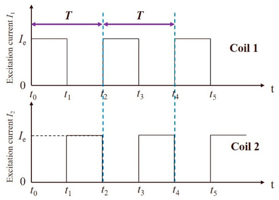
Figure 2.
Waveform of the excitation current.
Figure 3 shows the magnetic computational domain using coil 1 as an example. It mainly includes the magnetic generating device, workpiece, and magnetic field domain. The magnetic generating device is composed of an electromagnetic iron core and copper coils. The electromagnetic iron core is made from DT4C and its magnetic permeability curve is shown in Figure 4. The metal is 409L ferrite stainless steel and its magnetic permeability has a nonlinear response to temperature, as shown in Figure 5. When the temperature exceeds the Curie temperature of 770 °C, it transforms from ferromagnetic to superparamagnetic. There is a negative correlation between its permeability and temperature. It eventually approaches the permeability of vacuum. The temperature is much higher in the weld pool (>770 °C) than in the surrounding workpiece [16]. Thus, the upper part of the workpiece (−10 mm < z < −8 mm) is defined as the high-temperature region (>770 °C) and has a magnetic permeability of approximately 1. The remaining portion (−12 mm < z < −10 mm) is the relatively low-temperature region, and its magnetic permeability is 200. The other regions are defined as air with a relative permeability of 1 (the ratio of magnetic permeability to that of vacuum is 1), as shown in Figure 6.
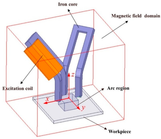
Figure 3.
Geometric model used to calculate external magnetic field.
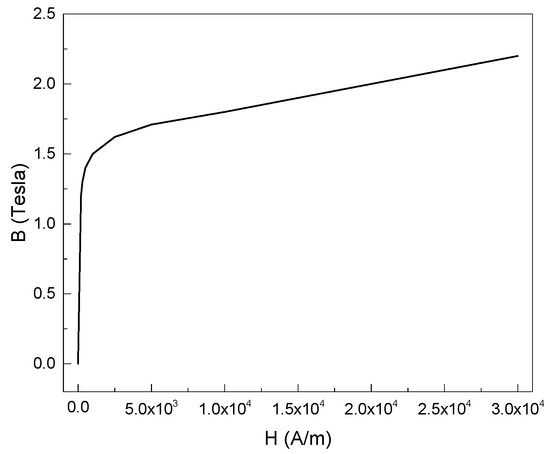
Figure 4.
Magnetization curve for DT4C.
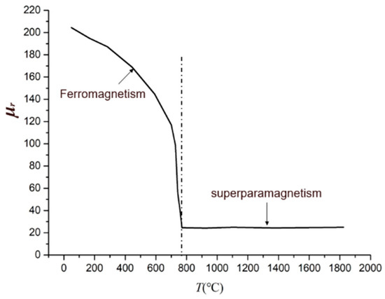
Figure 5.
409L T-permeability curve.
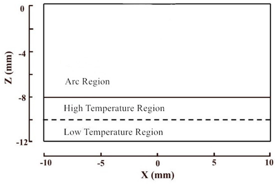
Figure 6.
Various regions in the model.
Figure 7 shows the three-dimensional magnetic field intensity distribution in the computation domain when coils 1 and 2 are energized using excitation currents of 3 A each. The lower face of the three magnetic poles in the excitation device presents a different polarity. Therefore, magnetic force lines are generated in various directions between the three magnetic poles. These are mainly concentrated around the iron core. The magnetic induction intensity is largest close to the magnetic poles. The maximum value is about 100 mT. Since the permeability of air is different from that of the workpiece, the internal magnetic induction intensity is also different. The magnetic field intensity in the arc and molten pool will be discussed later.
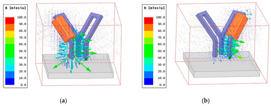
Figure 7.
Three-dimensional magnetic field intensity when (a) coil 1 and (b) coil 2 are energized.
3. Mathematical Model of GTAW with EMF
3.1. Basic Assumptions
To study interaction between the arc plasma, weld pool, metal vapor, and external composite magnetic field, the following assumptions were made when constructing mathematical models:
- The plasma arc is in local thermodynamic equilibrium (LTE) and is optically thin [17,18].
- The fluids in the plasma arc and weld pool are incompressible and their flows are laminar [19].
- The Boussinesq approximation can be used to treat the buoyancy force in the weld pool.
- The enthalpy porosity method can be used to handle the solid liquid mixing zone [20,21,22].
- Metal vapor particles are treated as the same gas and electrically neutral.
- The influence of the metal vapor on the molten pool quality can be ignored.
3.2. Governing Equations
The mass continuity equation is
The momentum equation is
where is the material density; p is the pressure; μ is the viscosity; u, v, and w are the velocity vectors in the x, y, and z directions, respectively; , , and are the self-induced electromagnetic force vectors in the x, y, and z directions, respectively; and , , and are the applied electromagnetic force vectors in the x, y, and z directions, respectively.
where , , and are the current density vectors; , , and are the self-induced magnetic field intensity components; and , , and are the additional magnetic field intensity components in the x, y, and z directions, respectively.
The energy conservation equation is
where is the additional energy source [23,24] and is the specific heat at constant pressure.
In the arc area,
where σ is the electrical conductivity; kb is the Boltzmann constant and is equal to 1.38 × 10⁻²³ J·K−1; e is the electron charge and is equal to 1.602 × 10⁻¹⁹ C; ε is the emissivity and is equal to 0.4 W·m−2·K; T0 is the indoor temperature which is 300 K in calculation; and α is the Stefan Boltzmann constant and is equal to 5.67 × 10⁻⁸ W·m−2·K−4.
In the workpiece area,
where ∆H is latent heat of fusion, f1 is the liquid fraction, Tl is the liquidus temperature, and TS is the solidus temperature [25].
The current continuity equation is
Ohm’s law is
The partial differential equations of the electromagnetic field are
The magnetic vector potential is
where is the potential, is the magnetic vector potential, and is the magnetic permeability, which equals 1.26 × 10⁻⁶.
The metal vapor transport equation is
where Ym is the mass fraction of metal vapor and D is the binary diffusion coefficient, which is defined as follows [26]:
where M1 and M2 are the molar masses of iron and argon atoms; , , , and are the density and viscosity of iron and argon, respectively; and and are dimensionless constants that equal 1.384.
3.3. Computation Domain and Boundary Conditions
The computation domain is shown as Figure 8. The GTAW welding gun nozzle diameter is 9.6 mm, the tungsten electrode is simplified into an inverted table shape with a tip diameter of 0.6 mm and an angle of 60 degrees, and the tungsten extreme part is 5 mm away from the workpiece. The workpiece is made from 4 mm-thick 409L stainless steel plate. Ar is used as the shielding gas and its flow rate is 20 L/min. Boundary conditions are shown in Table 1.
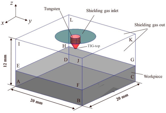
Figure 8.
Three-dimensional computation domain.

Table 1.
Boundary conditions.
3.4. Energy Terms at the Interface
The energy sources at the interface between the arc and tungsten electrode mainly include three parts: heat reduction caused by electron emission from the tungsten electrode, the energy released by the impact of positive ions on the tungsten electrode, and the heat loss caused by radiation from the tungsten electrode.
where je is the electron current density, φc is the tungsten material work function, ji is the ionic current density, and Vi is the ionization potential of argon, which equals 15.68 V.
The LTE-diffusion approximation method [27] is used to treat the interface between the weld pool and arc. The heat transferred from the arc to the workpiece mainly includes three parts: the electronic heat qe, the conduction heat qc, and the surface radiation heat qr.
where is the work function of steel and equals 4.65 V, K is the thermal conductivity, T is the temperature of the stainless steel surface, Te is the temperature of the arc next to the workpiece, δ is the thickness of the anode region and is taken as 0.2 mm, and is the emissivity of the anode material and equals 0.4 W·m−2·K.
3.5. Welding Parameters and Material Properties
The main welding parameters in this study are listed in Table 2.
Table 2.
Main welding parameters.
In the GTAW process, the thermodynamic and transport properties of argon, including its enthalpy, specific heat, density, viscosity, radiant heat, and electrical conductivity, are temperature dependent and are described in the literature [28]. The main physical parameters of 409L stainless steel used in this study are shown in Table 3.
Table 3.
Main physical properties of 409L stainless steel used in this model.
4. Results and Discussion
4.1. Magnetic Induction Intensity Distribution
Figure 9 and Figure 10 show the magnetic field intensity distributions on the xoz and yoz planes when coil 1 and coil 2 are respectively energized (the excitation current is 3 A). When coil 1 is deenergized and coil 2 is energized, the direction of the magnetic induction intensity on the xoz plane remains the same, as shown in Figure 9a and Figure 10a. However, the direction of the magnetic induction intensity on the yoz plane changes along the negative Y-axis to the positive Y-axis, as shown in Figure 9b and Figure 10b. Given the same excitation current, the magnetic field distribution is related to the distance between each point and the magnetic pole in the calculation domain. The maximum magnetic induction intensity of approximately 0.035 T occurs at the tungsten extreme part. The magnetic induction intensity is smaller (approximately 0.002–0.01 T) at points further from the tungsten extreme part in the arc region. In the workpiece region, the magnetic induction intensity in the region above the critical temperature (high-temperature region) is approximately 0.002–0.02 T, the magnetic permeability in the region below the critical temperature (low-temperature region) is relatively high, and the magnetic induction intensity is approximately 0.015–0.035 T.
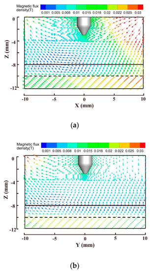
Figure 9.
EMF distributions when coil 1 is energized: (a) xoz and (b) yoz planes.
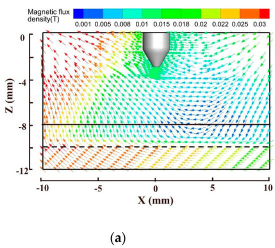
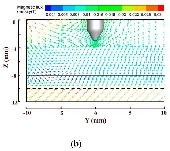
Figure 10.
EMF distributions when coil 2 is energized: (a) xoz and (b) yoz planes.
4.2. Effect on Arc-Pool Behavior
Figure 11 shows the calculated temperature and flow field of the TIG arc and weld pool at 0.4 s on the yoz and xoz planes before and after applying a magnetic field. When no compound magnetic field is applied, as shown in Figure 11a, the temperature and flow fields are symmetrical about the tungsten electrode axis. The maximum temperature of approximately 21,000 K occurs at the top of the tungsten electrode. Under the action of electromagnetic force, charged particles accelerate to the workpiece surface and then flow tangentially along it. The maximum axial flow velocity is 253 m/s. Under the action of surface tension, the high-temperature liquid metal on the molten pool surface flows from the center to the edge of the pool, and then flows along the solid liquid interface of the workpiece into the interior of the pool. Meanwhile, due to the arc pressure below the tungsten electrode and the self-induced electromagnetic force of the liquid metal, part of the liquid metal in the weld center flows downward from the weld pool center without moving to the edge of the weld. This transfers heat to the bottom of the weld pool and improves the weld depth.

Figure 11.
Temperature and flow field distributions: (a) Ie = 0 (yoz plane), (b) Ie = 3 A (yoz plane), and (c) Ie = 3 A (xoz plane).
When a compound magnetic field is applied, as shown in Figure 11b,c, the temperature and flow fields are no longer symmetrical about the tungsten electrode axis. The welding arc always leans forward in the forward direction of welding (yoz plane). Under the action of arc shear force and pressure, the surface liquid metal in front of the arc flows to the front of the weld pool and back to the weld center along the solid liquid interface. The maximum tangential velocity is 0.4 m/s. The flow rate inside the molten pool is 0.28 m/s. The surface liquid metal behind the arc flows from the center to the edge due to the action of surface tension, thus forming a long, shallow weld in the forward direction of welding. In the vertical welding direction (xoz plane), the shearing force of the welding arc has weak effects. Under the effect of surface tension, liquid metal flows from the weld center to the edge of the weld and flows back to the bottom of the weld center along the solid liquid interface. The flow of liquid metal forms a convective cycle, in which the flow rate of liquid metal in the molten pool is approximately 0.1 m/s.
Figure 12a shows current density distributions without external magnetic field (Ie = 0). The current density flows from the bottom of the workpiece to the tungsten electrode. This occurs primarily between the arc and the workpiece. As mentioned above, the arc keeps inclined forward in yoz plane but swings periodically in xoz plane when the external magnetic field is applied (Ie = 3 A). t1 means coil 1 is energized as shown in Figure 2 and t2 means coil 2 is energized in Figure 2. After the magnetic field is applied, the current density field changes from an axisymmetric distribution to an asymmetric distribution. Its deflection direction is the same as that of the arc and its size does not change substantially. The current density maximum in the arc region (approximately 2.2 × 10⁸ A/m2) occurs on the tungsten electrode surface. Moreover, the current density is smaller further from the tungsten pole. The current density in the arc column is within the range of 1 × 10⁶–5 × 10⁷ A/m2 and the maximum current density in the workpiece is 2 × 10⁶ A/m2.
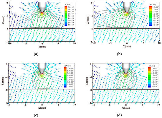
Figure 12.
Current density distributions: (a) Ie = 0 (yoz plane), (b) Ie = 3 A, t = t1 (yoz plane), (c) Ie = 3 A, t = t1 (xoz plane), and (d) Ie = 3 A, t = t2 (xoz plane).
Figure 13 shows the strength and distribution of the self-induced electromagnetic force. After applying the magnetic field, the self-induced electromagnetic force transitions from having a symmetrical distribution to exhibiting deviation from the tungsten electrode axis. It is then mainly concentrated between the arc and the workpiece. The field points to the center of the arc and workpiece from all sides, prompting the arc to contract inward and liquid metal in the molten pool to flow deep into the weld center. The maximum value of the self-induced electromagnetic force still occurs at top of the tungsten and does not change substantially. It remains approximately 2 × 10⁶ N/m3. The self-induced electromagnetic force is within the range of 5 × 10³–5 × 10⁵ N/m3 in the arc column area. Compared to other areas, the self-induced electromagnetic force in the workpiece area is relatively small at approximately 1000–5000 N/m3.
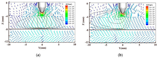
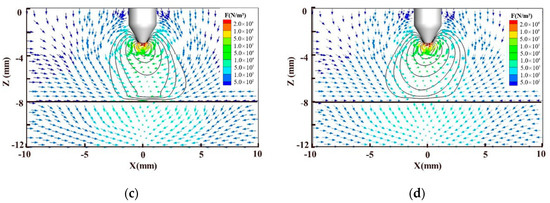
Figure 13.
Self-induced electromagnetic force: (a) Ie = 0 (yoz plane), (b) Ie = 3 A, t = t1 (yoz plane), (c) Ie = 3 A, t = t1 (xoz plane), and (d) Ie = 3 A, t = t2 (xoz plane).
Figure 14 shows the distribution of applied electromagnetic force. The applied electromagnetic force is generated via coupling between the applied external magnetic field and the current in the arc space. The applied electromagnetic force is distributed clockwise in the direction of welding, as well as alternately clockwise and counterclockwise in the direction of vertical welding. The external electromagnetic force is maximized at the tungsten electrode (approximately 2 × 10⁶ N/m3). The external electromagnetic force in the arc column area is within the range 5 × 10³–5 × 10⁵ N/m3. Because the workpiece has better magnetic permeability than air, the external electromagnetic force is stronger in the workpiece area than in the arc space. Its maximum is approximately 5 × 10⁴ N/m3. The external electromagnetic force in the molten pool is approximately 5000 N/m3.
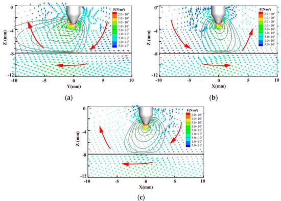
Figure 14.
Additional electromagnetic force: (a) Ie = 3 A, t = t1 (yoz plane), (b) Ie = 3 A, t = t1 (xoz plane), and (c) Ie = 3 A, t = t2 (xoz plane).
4.3. Effect of the Metal Vapor on Arc and Molten Pool Behavior
Figure 15a shows the welding temperature field and the metal vapor distribution across a cross section without a magnetic field. At 0.4 s, the liquid metal generates hot metal vapor. The metal vapor is primarily concentrated on the molten pool surface and diffuses to the surrounding space via convection and diffusion. Due to pressure from the arc plasma flow, diffusion of the metal vapor generated on the molten pool surface is hindered in the axial direction. In contrast, in the radial direction, the plasma flow pushes the metal vapor. Diffusion is intensified and flows out from the arc plasma boundary. The metal vapor content is maximized at approximately 0.8% near the center of the anode surface. Figure 15b,c show the metal vapor distribution with an external magnetic field. Compared to the result without an external magnetic field, arc deflection under the action of the external magnetic field causes the high-temperature area of the workpiece to deviate from the axis and the metal vapor to exhibit an asymmetric distribution. The deflection arc heats the workpiece area on the same side more intensively and the metal vapor content is higher than in other areas. The maximum metal vapor content in the yoz plane is approximately 0.6% and occurs on the negative Y-axis (−5 mm). In the xoz plane, the maximum metal vapor content is approximately 0.45% and occurs on the negative X-axis (−3 mm). In addition, the periodic swing of the arc reduces the molten pool surface temperature and the maximum amount of metal vapor generated on the molten pool surface decreases from 0.8% to 0.6%. This also weakens diffusion of metal vapor to the arc.
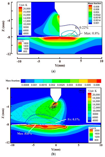
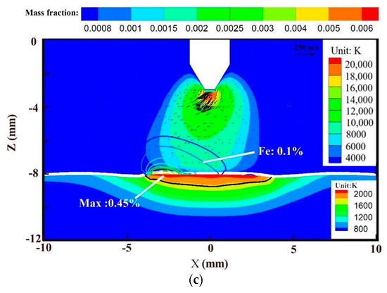
Figure 15.
Metal vapor distribution: (a) Ie = 0 A (yoz plane), (b) Ie = 3 A (yoz plane), and (c) Ie = 3 A (xoz plane).
Figure 16 shows the temperature field distribution of the arc with an external magnetic field under two conditions. The black full line represents the arc temperature field without considering the metal vapor and the red dotted line represents the arc temperature field with the effect of the metal vapor included. When the metal vapor is considered, the arc isotherm (4000–12,000 K) exhibits an obvious shrinkage phenomenon in area 1 where the metal vapor is concentrated. That is, the metal vapor reduces the temperature in the area around the arc. The arc does not exhibit shrinkage in area 2 where the metal vapor concentration is lower. The spread area (8000–20,000 K) of the arc on the upper workpiece surface is clearly reduced.
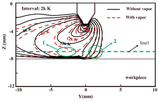
Figure 16.
Simulated arc temperature with EMF.
Figure 17 shows the arc temperature distribution, radiation loss, electrical conductivity, and current density distribution on a horizontal section (Line 1 in Figure 16) located 1 mm above the workpiece. According to Figure 17a, there is a large number of iron atoms in area 1 (−5 mm < y < 0 mm), where metal vapor is concentrated. Since iron atoms have a higher radiation coefficient than argon atoms, this increases radiation loss and reduces the arc temperature. Compared to the same area when no metal vapor is added, the arc temperature differs by approximately 2500 K. According to Figure 17b–d, the decreased arc temperature decreases the conductivity in area 1. Although the electrical conductivity of Fe atoms is higher than that of Ar atoms and the presence of Fe increases the conductivity in this area to some extent, this paper considers that the electrical conductivity decrease caused by the lower arc temperature is larger than the increase caused by aggregation of Fe atoms. Thus, the overall electric conductivity in area 1 exhibits a macroscopic decreasing trend. The decreased electrical conductivity leads to a decreased current density in area 1. The decreased current density makes the temperature of the arc even worse. In contrast, area 2 (0 mm < y < 2 mm) has less metal vapor accumulation and slightly increased radiation loss, but the change in the arc temperature is negligible. This is because the presence of metal vapor increases the overall conductivity of area 2 slightly. The current density is increased, the extra Joule heat generated by the arc is offset by heat released via increased radiation loss, and the arc temperature remains unchanged. Another reason for the increased current density in area 2 is the principle of current conservation. The current density increases on both sides of the area where the current density decreases, so the current density in area 2 increases. In addition, the peak values of the physical parameters occur closer to the tungsten electrode axis than if the metal vapor is not considered.
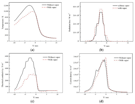
Figure 17.
Influence of the metal vapor on arc characteristics: (a) temperature, (b) radiation loss, (c) electrical conductivity, and (d) current density.
Metal vapor changes the thermal behavior of the arc, the heat flow and current density distributions on the workpiece surface, and finally the forming quality of the weld. Figure 18 shows the weld morphologies in the yoz and xoz planes with and without vapor. The arc shrinks in the forward direction of welding and the welding heat input is reduced when the vapor is considered. In the forward direction of welding (yoz plane), the heating area of the workpiece, the weld length on the negative Y-axis, and the weld depth decrease, while the weld length on the positive Y-axis increases. In the vertical welding direction (xoz plane), the weld width and depth increase primarily because the arc energy in the xoz plane is more concentrated due to shrinkage of the GTAW arc in the yoz plane relative to a system without metal vapor.
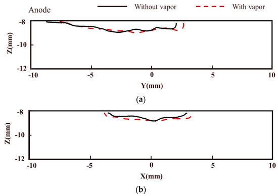
Figure 18.
Influence of metal vapor on pool morphology: (a) yoz and (b) xoz planes.
4.4. Experimental Validation
Overlay without wire filling was conducted to validate the numerical simulation results. The welding speed was 1 m/min and other welding parameters were same as the numerical simulation (Table 2). Figure 19 shows the schematic diagram of the experimental platform. Arc images were collected by two cameras along the welding direction and perpendicular to the welding direction, respectively.
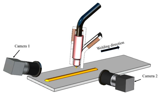
Figure 19.
The schematic diagram of experimental platform.
Figure 20 displays the arc behavior influenced by external magnetic field. When the excitation current was 3.0 A, the welding arc always tilted forward in the welding direction, and the arc turned left and right periodically in the vertical welding direction.
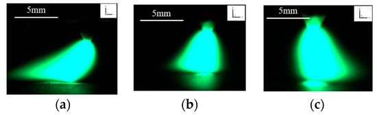
Figure 20.
The captured arc images: (a) by camera 2, (b) by camera 1, and (c) by camera 1.
Figure 21a shows the surface morphology of the welds without external magnetic field. There is sag in the welding toes, which is known as undercutting defect. Figure 21b shows the surface morphology after applying an external magnetic field. The undercutting defect was totally suppressed compared with Figure 21a. The experimental results indicated that the external magnetic field is beneficial to improve weld deformation for high-speed welding.
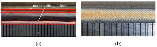
Figure 21.
The surface morphology of weld: (a) Ie = 0 and (b) Ie = 3 A.
The TD8620 handheld digital tesla meter was employed to test the experimental value of the external magnetic field. The magnetic flux density on the lower surfaces of two iron cores (wrapped by coils) were measured when the coil 1 was energized at different levels of excitation current (2–10 A). The comparison between the simulated and experimental results is shown in Figure 22. It indicates that the simulated values have good agreements with the measurement results.
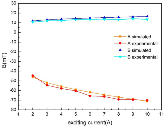
Figure 22.
Comparison between simulated and experimental value of magnetic field.
In order to verify the numerical simulation results, this study used the Boltzmann plot method to acquire temperature distributions. The Boltzmann plot method, also known as the multispectral method, is a temperature measurement method used to determine plasma temperatures by measuring the relative strengths of multiple spectral lines. The formula is as follows:
where I is the relative strength, λ is the wavelength, A is the transition probability, g is the degeneracy, E is the energy level, and k is the Boltzmann constant. I and λ are obtained experimentally, while A, g, and E are obtained from the National Institute of Standards and Technology database [29].
The arc plasma measurement platform includes a three-dimensional motion platform and a fiber-optic spectrometer, as shown in Figure 23. The optical fiber probe is driven by the mobile platform to collect an arc spectrum at fixed point in space. During the experiment, the arc is divided into six layers and 20 points are collected from each layer, as shown in Figure 24. The spectral data from these points are calculated to determine the temperature at each point.

Figure 23.
The measurement platform. (a) Three-dimensional motion platform and (b) fiber-optic spectrometer.
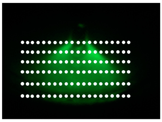
Figure 24.
Distribution of collection points.
Figure 25 compares the simulated and experimental results. The simulated result (left) nearly matches the experimental result (right).
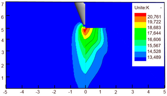
Figure 25.
Arc temperature distribution in the simulated and experimental results.
Figure 26a shows arc shape images determined via magnetron welding testing, while Figure 26b shows arc morphologies obtained via simulation using the same process parameters. The simulation results are in good agreement with the experimental results.
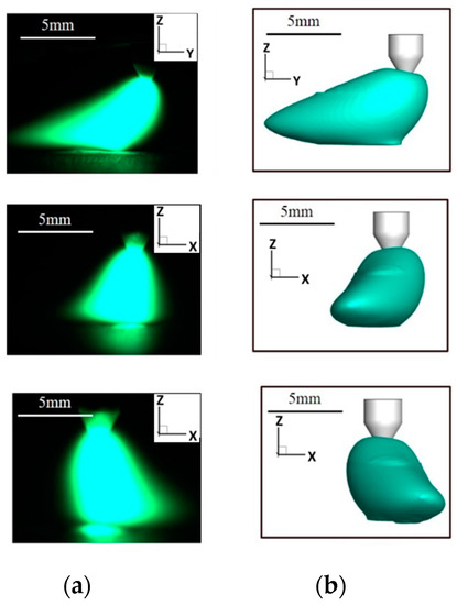
Figure 26.
Arc shape image: (a) experiment and (b) simulation.
Table 4 compares actual and simulated arc and deflection angles under various excitation currents. The forward and deflection angles are in good agreement. This also verifies the reliability of the numerical model.
Table 4.
Comparison of experimentally determined and simulated arc inclination angles.
5. Conclusions
- A three-dimensional numerical calculation model of an external compound magnetic field was established using a magnetic generator. The magnetic field distribution in the arc and workpiece was simulated using ANSYS software. The magnetic field intensity of the lower end of the magnetic pole was measured. A comparison shows that the results are in good agreement. This verifies the reliability of the numerical model.
- After the magnetic field is applied, the physical fields in the calculation domain are not symmetric along the tungsten electrode axis. The peak arc temperature is unchanged and the velocity decreases. Under the action of arc shear force and pressure, the metal on the weld pool surface flows to the front of the weld and then flows back to the center of the weld. The additional electromagnetic force is the main driving force for arc deflection, which has little effect on metal flow in the molten pool.
- A mathematical model of metal vapor was established. The deflection arc caused the high-temperature area of the workpiece to deviate from the tungsten electrode axis and the metal vapor exhibited an asymmetric distribution. The periodic swing of the arc reduced the welding heat input and the amount of metal vapor produced, as well as weakening its diffusion to the arc area. In the area where metal vapor was concentrated, the arc isotherms shrank and the temperature decreased by approximately 2500 K. In the area with less metal vapor, the arc temperature was basically unchanged. In the forward direction of welding (yoz plane), shrinkage of the welding arc led to a decrease in the workpiece heating area and a slight decrease in the melting depth. The melting width and the melting depth were increased in the vertical welding direction (xoz plane).
Author Contributions
Conceptualization, J.C.; validation, Y.H.; formal analysis, Y.H. and L.L.; original draft preparation, L.L. and Y.H.; review and editing, Y.H., J.C., L.W. and C.W. All authors have read and agreed to the published version of the manuscript.
Funding
This research was funded by National Natural Science Foundation of China (No. 51775313), Major Program of Shandong Province Natural Science Foundation (No. ZR2018ZC1760), and Young Scholars Program of Shandong University (No. 2017WLJH24).
Conflicts of Interest
The authors declare no conflict of interest.
References
- Yang, Z.; Cheng, Z. Development and application of new varieties of ultrapure ferrite stainless steel. China Metall. 2013, 23, 17–21. [Google Scholar]
- Chang, Y.; Gao, F.; Lu, L.; Gao, Y.; Liu, X. Research status and development trend of TIG welding technology. In Proceedings of the Forum on Development of Welding and Coating Technology in China Shipping and Marine Engineering, Guangzhou, China, 22 November 2012; pp. 33–38. [Google Scholar]
- Wu, H.; Chang, Y.; Lu, L.; Bai, J. Review on magnetically controlled arc welding process. Int. J. Adv. Manuf. Technol. 2017, 91, 4263–4273. [Google Scholar] [CrossRef]
- Li, T. Research status of electromagnetic field assisted welding technology. Welding 2017, 10, 18–24. [Google Scholar]
- Hicken, G.K.J.C.E. Effects of applied magnetic fields on welding arcs. Weld. J. 1966, 45, 515–525. [Google Scholar]
- Ando, K.; Nishikawa, J.; Yamanouchi, N. Effects of the magnetic field on bead formation in TIG arc welding. J. Jpn. Weld. Soc. 1968, 37, 41–50. [Google Scholar] [CrossRef][Green Version]
- Ukita, S.; Kokubo, K.; Masuko, T.; Irie, T. High-speed DCEN TIG welding of very thin aluminium sheets with magnetic arc control. Weld. Int. 2003, 17, 541–549. [Google Scholar] [CrossRef]
- Pearce, B.P.; Kerr, H.W. Grain refinement in magnetically stirred GTA welds of aluminum alloys. Met. Mater. Trans. A 1981, 12, 479–486. [Google Scholar] [CrossRef]
- Jiang, C. Numerical Analysis of Thermal and Force Characteristics of MIG Arc under externally Applied Magnetic Field. Master’s Thesis, Shandong University, Jinan, China, 1 May 2019. [Google Scholar]
- Xiao, L.; Fan, D.; Huang, J. Three-dimensional numerical analysis of the interaction between a fixed point active tungsten inert gas arc welding and a molten pool. Chin. J. Mech. Eng. 2016, 52, 93–99. [Google Scholar] [CrossRef]
- Wang, C. Numerical Simulation of Temperature Field and Flow in TIG Welding Pool under Longitudinal Magnetic Field. Master’s Thesis, Chongqing University, Chongqing, China, 1 May 2014. [Google Scholar]
- Bachmann, M.; Avilov, V.; Gumenyuk, A.; Rethmeier, M. About the influence of a steady magnetic field on weld pool dynamics in partial penetration high power laser beam welding of thick aluminium parts. Int. J. Heat Mass Transf. 2013, 60, 309–321. [Google Scholar] [CrossRef]
- Tanaka, M.; Yamamoto, K.; Tashiro, S.; Nakata, K.; Yamamoto, E.; Yamazaki, K.; Suzuki, K.; Murphy, A.B.; Lowke, J. Time-dependent calculations of molten pool formation and thermal plasma with metal vapor in gas tungsten arc welding. J. Phys. D Appl. Phys. 2010, 43, 434009. [Google Scholar] [CrossRef]
- Jian, X.X.; Wu, C.S. Influence of Fe vapor on plasma arc welding molten pool behavior. Acta Metall. 2016, 52, 1467–1476. [Google Scholar]
- Kim, W.-H.; Fan, H.G.; Na, S.-J. Effect of various driving forces on heat and mass transfer in arc welding. Numer. Heat Transf. Part A Appl. 1997, 32, 633–652. [Google Scholar] [CrossRef]
- Li, Y. Numerical Analysis of Applied Electromagnetic Field Used to Regulate the Liquid Flow toward the Rear of High-Speed GMAW Molten Pool. Master’s Thesis, Shandong University, Jinan, China, 1 May 2015. [Google Scholar]
- Tanaka, M.; Lowke, J.J. Predictions of weld pool profiles using plasma physics. J. Phys. D Appl. Phys. 2006, 40, R1–R23. [Google Scholar] [CrossRef]
- Guo, Z.; Zhao, W. Arc and Thermal Plasma; Science Press: Beijing, China, 1986. [Google Scholar]
- Kim, W.-H.; Na, S.-J. Heat and fluid flow in pulsed current GTA weld pool. Int. J. Heat Mass Transf. 1998, 41, 3213–3227. [Google Scholar] [CrossRef]
- Pan, J. Numerical Analysis of Arc and Pool Characteristics of Nonmelting Polar Variable Polarity Welding of Aluminum Alloy. Ph.D. Thesis, Tianjin University, Tianjin, China, 1 December 2016. [Google Scholar]
- Voller, V.; Prakash, C. A fixed grid numerical modelling methodology for convection-diffusion mushy region phase-change problems. Int. J. Heat Mass Transf. 1987, 30, 1709–1719. [Google Scholar] [CrossRef]
- Prakash, C.; Voller, V. On the numerical solution of continuum mixture model equations describing binary solid-liquid phase change. Numer. Heat Transfer Part B Fundam. 1989, 15, 171–189. [Google Scholar] [CrossRef]
- Lu, F.; Wang, H.-P.; Murphy, A.B.; Carlson, B.E. Analysis of energy flow in gas metal arc welding processes through self-consistent three-dimensional process simulation. Int. J. Heat Mass Transf. 2014, 68, 215–223. [Google Scholar] [CrossRef]
- Tashiro, S.; Miyata, M.; Tanaka, M. Numerical analysis of AC tungsten inert gas welding of aluminum plate in consideration of oxide layer cleaning. Thin Solid Films 2011, 519, 7025–7029. [Google Scholar] [CrossRef]
- Jian, X.X.; Wu, C.S. Determination of arc pressure and current density on the molten pool surface in plasma arc welding. China Weld. (Eng. Ed.) 2014, 23, 78–82. [Google Scholar]
- Heberlein, J.; Murphy, A.B. Thermal plasma waste treatment. J. Phys. D Appl. Phys. 2008, 41, 053001. [Google Scholar] [CrossRef]
- Lowke, J.J.; Tanaka, M. ‘LTE-diffusion approximation’ for arc calculations. J. Phys. D Appl. Phys. 2006, 39, 3634. [Google Scholar] [CrossRef]
- Murphy, A.B. The effects of metal vapour in arc welding. J. Phys. D Appl. Phys. 2010, 43, 434001. [Google Scholar] [CrossRef]
- NIST Atomic Spectra Database Lines Form. Available online: https://physics.nist.gov/PhysRefData/ASD/lines_form.html (accessed on 30 June 2020).


© 2020 by the authors. Licensee MDPI, Basel, Switzerland. This article is an open access article distributed under the terms and conditions of the Creative Commons Attribution (CC BY) license (http://creativecommons.org/licenses/by/4.0/).