Abstract
In this investigation, three-dimensional molecular dynamics simulations have been performed in order to investigate the effects of the workpiece subsurface temperature on various nanocutting process parameters including cutting forces, friction coefficient, as well as the distribution of temperature and equivalent Von Mises stress at the subsurface. The simulation domain consists of a tool with a negative rake angle made of diamond and a workpiece made of copper. The grinding speed was considered equal to 100 m/s, while the depth of cut was set to 2 nm. The obtained results suggest that the subsurface temperature significantly affects all of the aforementioned nanocutting process parameters. More specifically, it has been numerically validated that, for high subsurface temperature values, thermal softening becomes dominant and this results in the reduction of the cutting forces. Finally, the dependency of local properties of the workpiece material, such as thermal conductivity and residual stresses on the subsurface temperature has been captured using numerical simulations for the first time to the authors’ best knowledge.
1. Introduction
Nano/micro-cutting is a term widely used to describe material removal at nanoscale. Nanocutting processes are characterised by the high-speed of the cutting tool as well as their ultra-precision. Nowadays, nanoscale machining processes are playing an essential role in the modern manufacturing industry, while numerous investigations on the topic have been performed since the late 1990s. Machining processes at the nanoscale can be grouped in four categories depending on their applications: (a) deterministic mechanical nanometric machining, (b) loose abrasive nanometric machining, (c) non-mechanical nanometric machining, and (d) lithographic method [1]. Mechanical nanometric machining appears to be the more advantageous among its alternatives, as it allows for the machining of complex 3D shapes, while the cutting accuracy can reach tens on nanometers [2,3]. Moreover, as advocated by Stephenson et al. [4], who investigated the nano-grinding process of hard steel using a 76 µm cubic boron nitride (CBN) grit with a depth of cut set equal to 500 µm, nanometric machining can generate very smooth and repeatable surface finish (Ra < 10 nm).
Over the course of time, the development of high-performance computers (HPCs) has contributed to the advancement of nanotechnology [5]. The evolution of HPC facilities has allowed for very computationally expensive simulations. Three of the most important numerical modelling techniques in terms of mechanics and thermodynamics are (a) kinematic models, (b) finite element analysis (FEA), and (c) molecular dynamics (MD) simulations. Kinematic and FEA models can be used for the estimation of the physical characteristics, such as the cutting forces and temperature in two different scales, i.e., macroscale [6] and microscale [7]. Notwithstanding the above, recent studies on kinematic [8] and FEA models [9] have shown the limitations of the aforementioned modelling techniques with respect to their accuracy. Their poor accuracy when approaching micro- and nanoscale is due to the fact that in such small scales the surface-area-to-volume ratio increases; consequently, surface phenomena become increasingly dominant [10].
On the other hand, the MD simulations method is based on the calculation of the atoms’ trajectories using Newton’s equation of motion in order to extract meaningful properties of materials and investigate physical phenomena. In addition, MD simulations can provide high-resolution information and require no ab initio assumptions in contrast to kinematic models and FEA. MD simulations have often been utilised in research investigations during the last couple of decades due to their capability of capturing atomistic details [11,12,13]. Many researchers have used MD simulations for several applications, such as crack propagation [14], nanoflows [15], and defect formation in nanocutting [16,17] in order to understand the corresponding phenomena at the nanoscale level. Since this study will be focusing on nanoscale phenomena during the nanocutting process, MD has been selected as the most suitable modelling technique among the alternative options.
Pioneering MD investigations were focused on nanocutting of copper, aluminium, and silicon workpieces with different grinding speeds ranging between 100 and 500 m/s and various tool sizes and geometries [18]. Inamura et al. [19] evaluated the 2D nanoscale cutting interaction between a copper workpiece and a diamond tool. They showed that the cutting process is affected by the interaction between the tool and workpiece atoms. One of the most investigated topics related to nanocutting phenomena is the effect of the tool geometry on the grinding mechanics [20]. Xie and Fang [21] conducted an investigation, which was mainly focused on the effects of the cutting-edge radius on the chip formation, cutting forces, and stress distribution at atomic and close-to-atomic scales (ACS). Since conventional continuum mechanics could be no longer applied, they proposed a study to verify the mechanism employed at the ACS process. Due to the fact that the material removal mechanism at ACS remains unclear, it is still difficult to increase the machining accuracy from nanoscale to atomic scale. The authors demonstrated that, with an ACS cutting depth of 1 nm, the minimum chip thickness could be down to a single atomic layer. As a consequence, the ACS cutting process was found to be affected by two sizing effects, namely the cutting radius size effect and the atomic sizing effect. Moreover, it was found that it is necessary to control with extreme accuracy the movement of the atomic layers in order to avoid surface deformities at ACS. In another study, Rentsh and Inasaki [22,23] employed MD simulations in order to shed light on the dislocation generation, surface roughness, residual stresses, and crack propagation. Overall, MD has been widely used for studying manufacturing processes [24,25], while the number of published papers per year implementing this technique is continuously increasing.
Previous MD simulations have shown that there are several key parameters with a significant impact on the nanocutting mechanism. According to [26], the workpiece temperature in the grinding process is affected by many factors, including the workpiece material, the tool material, application of grinding fluid, grinding speed, and wheel dressing conditions. Early studies on thermal modelling of grinding processes focused on conventional grinding and high efficiency deep grinding (HEDG), which had some significant limitations on the depth of cut—which ranged between 0.2 and 25 mm or more—the wheel, and workpiece speed [27,28]. Following these first studies, Werner et al. [29] attempted to model the heat flow to the workpiece, tool, chip, and fluid in creep feed grinding using FEA. Rowe, Black, and Morgan [30,31] investigated critical temperatures for the onset of thermal damage for several ferrous materials. In a recent study, Romero et al. [32] analysed the temperature distribution over an orthogonal cutting tool during nanocutting. In another study, Li at al. [33] demonstrated that the smaller depth of cut reduces subsurface damage, improves the grinding efficiency, and reduces energy consumption.
Based on the above, it is evident that the thermal effects on nanocutting have not been rigorously analysed yet in the atomic scale. This investigation is focused on the effects of the workpiece temperature on the nanocutting mechanism. The current analysis has been carried out with the aid of three-dimensional molecular dynamics (MD) simulations. The effects of the workpiece temperature on the cutting forces (Fx and Fy), friction factor (η), and the temperature distribution at the cutting area will be analysed and discussed. In addition, equivalent Von Misses stresses have been calculated over the simulation domain to analyse the stress distribution over the workpiece. The comparison of the obtained results provides us with a new point of view of the behaviour of the workpiece material with respect to yield strength and fracture toughness. The large-scale atomic/molecular massively parallel simulator LAMMPS (version 16 May 2018, Sandia National Laboratories, Albuquerque, NM, USA) [34] has been used for the completion of the simulations of this study and the OVITO software (Release 3.1.0, OVITO GmbH, Amtsgericht Darmstadt, Germany) has been used to visualise and analyse the atomistic output data [35].
2. Methodology
An MD simulation model has been developed for the purposes of this study. The MD simulation domain consists of a cutting tool made of diamond and a copper workpiece. The cutting tool was modelled as a convex isosceles trapezoid with a negative rake angle equal to −45°, which is much below the critical value for chip formation (≈−60°) [36]. The system contains 723,118 atoms, while the copper workpiece and diamond tool parameters are listed in Table 1. According to [37], the lattice constant of diamond is equal to 3.57 Å, and the lattice constant of face centred cubic (FCC) copper is equal to 3.597 Å. Both materials, diamond and copper, contain three zones with three types of atoms correspondingly: boundary atoms (dark blue zone), which consists of atom layers to ensure stability and prevent unwanted rigid body motion of the workpiece; Langevin thermostat atoms (red zone), which are used to control the temperature during the process, and Newtonian atoms (light blue zone), which correspond to the deformable zone [38], as shown in Figure 1.

Table 1.
Component properties.
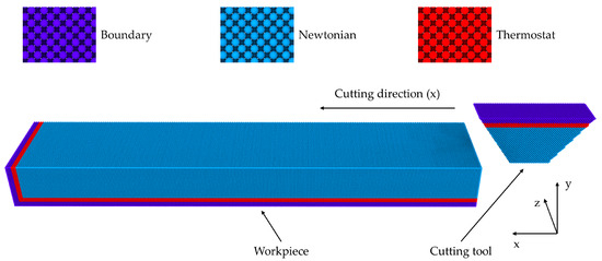
Figure 1.
Molecular dynamics (MD) simulation domain.
For the purposes of this study, the boundary atoms of the tool and the workpiece are assumed to be rigid, i.e., there is no relative dislocation between them. The fixed atoms of the workpiece are fixed to their initial positions, whilst the fixed atoms of the tool are assigned with a constant speed after the equilibration phase has been completed. The motion of the Newtonian and thermostat atoms is dictated by Newton’s second law of motion [39] and Brownian dynamics, respectively (Langevin thermostat). During the equilibration phase, the system was relaxed over 20,000 timesteps in order to achieve a constant pressure and temperature across the simulation domain. Following the equilibration phase, the tool boundary atoms started moving with a constant speed of 100 m/s, while the tool thermostat temperature has been set equal to different temperature values depending on the case under examination, namely (a) 300 K, (b) 500 K, (c) 700 K, and (d) 900 K. Finally, the cutting direction was coincident with the x-axis [100] direction, which corresponded to the (0 0 1) plane of the workpiece in the simulation. The atom positions were time-integrated with a timestep equal to 1.5 fs. All simulations were run with the system controlled by the microcanonical (NVE) ensemble.
There are 3 different types at the atomic level in the MD simulation domain: (1) the interaction between workpiece copper atoms (Cu–Cu), (2) the interaction between the tool diamond atoms (C–C), and (3) the interaction between workpiece and tool atoms (Cu–C). First, the interaction between copper workpiece atoms has been described using the embedded atom model (EAM) by Foiles et al. [40], which can be expressed as follows:
In the expression above, the total energy Etot is the sum of the individual embedding energy F and pair potential function φ(rij) representing the energy in bond ij, which is due to the short-range electro-static interaction between atoms. The indices i and j refer to the atoms i and j, respectively, rij is the interatomic distance, and φi is the electron density of the atom i. The host electron density can be approached by the superposition of atomic densities:
where ρja is the electron density contributed by the atom j. Secondly, the interaction between the diamond tool atoms has been modelled with the Tersoff potential [41] as follows:
In Equation (3), E is the total energy of the system, Vij the bond energy between atoms i and j, fA and fR are the attractive and repulsive terms, respectively, and bij is the bond order term. The cut-off function fC, given by Equation (4), is used to constrain the interaction forces within a specific distance range [R − D, R + D] with R, D constants selected to include only neighbouring cells.
Finally, the Morse potential was adopted to describe the interactions between the copper and diamond atoms of the workpiece and the tool, respectively [42]:
where E is the pair interaction energy, D0 = 0.087 eV the cohesion energy, a = 5.14 Å−1 elastic modulus, and r0 = 2.05 Å the equilibrium distance.
In this investigation, the focus was placed on the impact of the workpiece temperature on the nanocutting process characteristics. Four initial workpiece temperatures were considered, namely (a) 300 K, (b) 500 K, (c) 700 K, and (d) 900 K. In order to study the nanocutting behaviour of the copper workpiece at different initial temperatures and eliminate any statistical errors, 3 grinding simulations were performed for each case with random initial conditions. Moreover, the depth of cut was set equal to dc = 20 Å and remained constant during the grinding process so as to ensure that there is perfect contact between the two rigid bodies (workpiece and tool).
3. Results
In this section, the obtained results on the effects of the workpiece temperature on the (1) cutting forces, (2) friction factor, (3) subsurface temperature, and (4) Von Mises stresses will be thoroughly analysed and discussed. For the purposes of this analysis, four workpiece temperatures have been considered: (a) 300 K, (b) 500 K, (c), 700 K, and (d) 900 K.
3.1. Cutting Forces
Figure 2 shows the evolution of the cutting forces over time for a single MD simulation at different initial workpiece temperatures. The grinding force values were evaluated during the cutting phase of each simulation. Overall, it can be observed that the cutting forces decrease with the workpiece temperature. This is due to the fact that the copper workpiece loses gradually its mechanical strength due to thermal softening [43]. At the beginning of the grinding process, both cutting forces experienced a gradual and approximately linear increase in the time range [0 ps–150 ps] until they reach an approximately constant value. This occurred because at the beginning of the cutting process, there is no perfect contact between the tool and the workpiece. When both pieces are in perfect contact (t > 150 ps), both forces start to fluctuate around a constant value. Moreover, it can be observed that there is a gradual increase in both cutting forces due to the accumulation of chip at the front of the tool. This phenomenon has been visualised in Figure 2. A previous study showed that the tangential force is affected by the material pile-up in the direction of the x-axis, which coincides with the cutting direction [20]. As expected, it can be seen that in the Figure 3a, there is a large difference between the average values of the two cutting forces. Fx obtains a value about equal to 375 nN, while Fy reaches a value close to 250 nN. It can also be observed that the difference between the tangential and normal forces becomes smaller as the workpiece temperature increases. Furthermore, the normal force fluctuations increase with the workpiece temperature, i.e., Figure 3d is characterised by a higher fluctuation amplitude compared to the rest of the cases. According to Lin et al. [44], the large oscillations of cutting forces in the grinding process are related to the generation of dislocations.
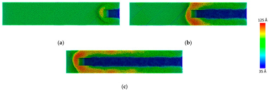
Figure 2.
Material pile-up at (a) 120 ps, (b) 360 ps, and (c) 660 ps.
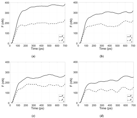
Figure 3.
Forces vs. time for (a) Tw = 300 K, (b) Tw = 500 K, (c) Tw = 700 K, and (d) Tw = 900 K.
However, the graphs above correspond to just one case, which might incur statistical inaccuracies. In order to avoid these statistical errors, three simulations were performed for each simulation case, and the average force values in the range of [100 ps–700 ps] were plotted against the workpiece temperature. In Figure 4, it is obvious that both cutting forces are characterised by a descending trend in accordance to the one identified in Figure 2. Therefore, the decrease in Fx and Fy is attributed to the increase the initial temperature of the workpiece due to thermal softening. This is also in agreement with previous numerical and experimental studies [43,45]. From Figure 4a, it can be observed that Fx decreases linearly with the workpiece temperature. On the contrary, Fy (Figure 4b) appears to decrease with a steeper slope, as the workpiece temperature rises above 500 K. These observations are in agreement with previous investigations [46,47] advocating that the yield strength and fracture toughness of copper decrease with increasing temperature on the workpiece. Moreover, it has been shown that the tensile ductility of copper exhibits a strong temperature dependence [48].
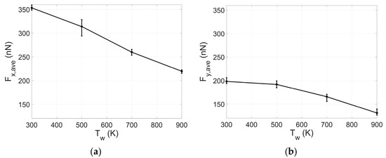
Figure 4.
Cutting forces vs. workpiece temperature: (a) tangential forces (Fx) and (b) normal forces (Fy).
3.2. Friction Factor
The dependence of the average friction factor ηave on the workpiece temperature has been plotted in Figure 5. For this purpose, the average friction factor has been expressed as the time average of the ratio of tangential to normal cutting forces during the cutting phase as follows:
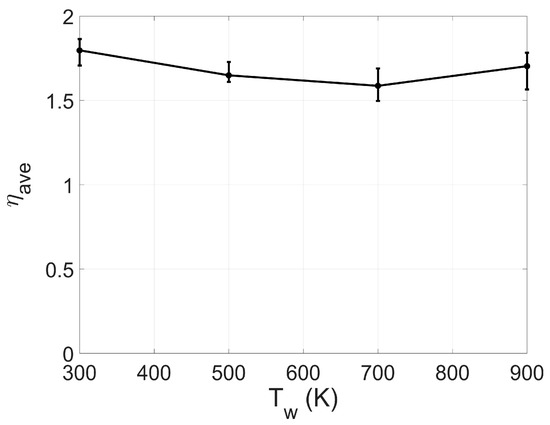
Figure 5.
Average friction factor vs. workpiece temperature.
In accordance to the trend of the averages of cutting forces, friction factor oscillated around values close to 1.7 within the workpiece temperature range [300 K–900 K]. Such trends are common in MD studies. It has to be noted that friction factor values higher than 1 are common in MD simulations; this is attributed to the material pile-up at the front of the tool [49,50].
3.3. Subsurface Temperature
It is well known that the mechanical properties of a material are significantly affected by the local temperature [51]. One important parameter during the grinding process is the workpiece subsurface temperature at the vicinity of the cutting tool. In order to measure the subsurface temperature at the cutting region, a spherical area with a radius equal to 15 Å was fixed at the centre of the lower (small) side of the trapezoidal cutting tool. This sphere overlapped with the workpiece atoms during the nanocutting process. The temperature of the workpiece atoms lying at this region was averaged over time windows of 30 ps in order to eliminate noise, while the workpiece atoms lying within the sphere were updated every 1 timestep (1.5 fs). The temperature at the cutting area was calculated as follows [25]:
In Equation (7), Tca is the workpiece temperature at the cutting area (ca), KE is the total kinetic energy of the group of atoms in the spherical region, mi the mass of atom i, dim = 1 the number of velocity components used for the evaluation of the kinetic energy, N the total number of workpiece atoms in the group, and kB = 1.38 10−23 m2 kg s−2 K−1 is the Boltzmann constant. Since the x and y component of the atoms’ velocities are associated with the translational motion of the cutting tool, only the z component (vz) was taken into consideration for the estimation of the abrasive temperature, as shown in Equation (7).
As expected, the temperature at the cutting area increases with the workpiece temperature. Figure 6 illustrates the evolution of the temperature of the cutting area over time during the nanocutting process. Overall, the temperature at the cutting area increases with the workpiece temperature over time. Similar to the cutting forces aforementioned, the Tca increases linearly during the first 150 ps for nanocutting grinding simulation. This is because the two components (tool and workpiece) are not in perfect contact during this time interval. Following the linear increase Tca reaches a constant value and fluctuates around this for the rest of the simulation.
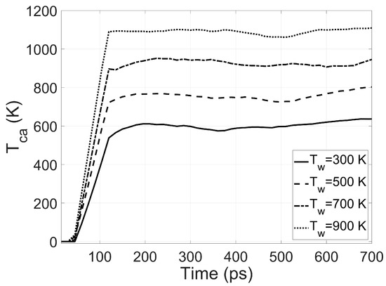
Figure 6.
Temperature at the cutting area (Tca) vs. time for various values of the workpiece temperature (Tw).
The dependence of the average temperature at the cutting area on the workpiece temperature is illustrated in Figure 7, where the average of Tca was estimated over three MD simulations in order to eliminate statistical errors. Overall, the graph describes an upward trend of Tca with respect to Tw as expected. More specifically, it can be observed that Tca increases approximately but not linearly with Tw; the difference Tca–Tw reduces for higher values of Tw. This observation will be further analysed in the following paragraphs.
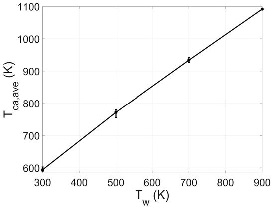
Figure 7.
Average temperature at the cutting area (Tca,ave) vs. workpiece temperature (Tw).
In order to enhance our understanding of the subsurface temperature distribution, the per-atom temperature of the workpiece atoms was visualised in Figure 8 for various initial workpiece temperature values, namely (a) 300 K, (b) 500 K, (c) 700 K, and (d) 900 K. In Figure 8, only half of the workpiece atoms are visible (cross section at zmid), while the tool atoms have been made transparent in order to enhance clarity. It can be observed that the temperature of the boundary atoms is equal to 0 K (dark blue zone), since they are rigid and do not get time-integrated. From Figure 8, it is evident that the higher temperature area is located at the contact area between the tool and the workpiece as expected. In Figure 8d, it can be seen that the temperature of the workpiece atoms reaches 1300 K. This fact is significant, since these atoms reach a temperature close to the melting point of copper and thermal softening becomes dominant. As a result, chip thickness increases for higher initial workpiece temperature values, as shown in Figure 8. At this point, it has to be noted that the fact that the height of the workpiece is only 70 Å. As a matter of fact, the cutting region is quite close to the thermostat and fixed atom layers of the workpiece, as shown in Figure 8; this might lead to an underestimation of the temperature values at the cutting area (Tca).
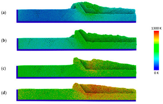
Figure 8.
Workpiece temperature distribution for (a) Tw = 300 K, (b) Tw = 500 K, (c) Tw = 700 K, and (d) Tw = 900 K.
Finally, in order to understand the reason behind the non-linear relationship between Tca and Tw, as illustrated in Figure 7, we analysed the behaviour of the surface temperature in a specific region (R) of the workpiece copper for various workpiece initial temperatures, such as 300 K, 500 K, 700 K, and 900 K. The location of the region R is illustrated in Figure 9. This region was defined by the area between x = 0 Å to x = 100 Å. It has to be noted that region R did not include the rigid atoms of the workpiece in the thermostat and rigid region in order to prevent miscalculation of temperature.
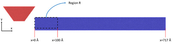
Figure 9.
Location of region R.
Figure 10a illustrates the evolution of the average temperature of the workpiece atoms lying in region R (TR). It can be observed that the trends of the temperature curves are similar, but not identical. In the beginning, TR increases gradually until it reaches a specific value and subsequently decreases. The increase of TR is due to the approach of the cutting tool, which elevates the local temperature. TR subsequently decreases, while the induced heat is dissipated as the tool moves away of the region. The most significant difference between the TR curves is their slopes. In order to investigate the non-linear relationship between the temperature at the cutting region and the subsurface temperature, the difference between the temperature of region R and the workpiece temperature (TR − Tw) has been plotted in Figure 10b as a function of time. It is clear that as the workpiece subsurface temperature increases the slope of TR − Tw becomes smoother, i.e., the response of TR is slower. Therefore, it can be concluded that there is a delay in the cooling process of this material for higher Tw values. The slower response of TR for higher workpiece temperatures occurs due to the decrease of the local thermal conductivity for higher temperature values. Therefore, due to the lower thermal conductivity, there is a decrease in the heat dissipation rate, which slows down the response of TR. This is the reason for the gradual reduction of the difference Tca,ave − Tw for higher workpiece temperature, as illustrated in Figure 7. This phenomenon has been observed for the first time using MD simulations, according to the authors’ best knowledge.
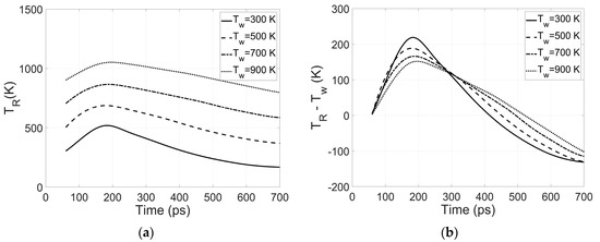
Figure 10.
(a) TR and (b) TR − Tw vs. time for various workpiece temperatures.
3.4. Equivalent Von Mises Stresses
In this section, the results on the equivalent Von Mises stresses (EVMS) distribution over the simulation domain will be presented. The equivalent Von Mises stress is given by:
where σVM is the equivalent Von Mises stress, σxx, σyy, and σzz are the normal stresses and σxy, σyz, and σzx the shear stresses, respectively. Figure 11 represents the Equivalent Von Mises stress (EVMS) distribution and the common neighbour analysis (CNA) of the workpiece for two extreme initial workpiece temperature svalues considered, i.e., Tw = 300 K and Tw = 900 K in order to highlight the effects workpiece temperature on the stress distribution. It can be observed that Figure 11a shows that there is high-stress concentration at the shear zone in contrast to Figure 11c. This is another observation related to the thermal softening of copper. Moreover, for elevated workpiece temperature, copper loses its mechanical strength, and the Von Mises stresses are more uniformly distributed across the workpiece. Moreover, by comparing EVMS and CNA in Figure 11, it can also be observed that there is high stress concentration at the vicinity of lattice dislocations, corresponding to hexagonal closed-packed (HCP) atoms, as expected. It should also be noted that high stress concentration is associated with dislocation generation and propagation.
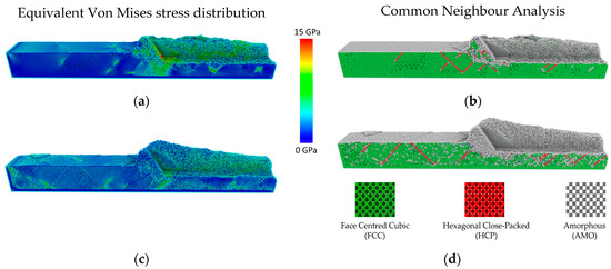
Figure 11.
Evolution of Von Mises distribution and common neighbour analysis for two workpiece temperature values: (a,b) Tw = 300 K and (c,d) Tw = 900 K.
4. Conclusions
In this study, the effects of the workpiece temperature on nanocutting phenomena have been investigated using molecular dynamics simulations. The process parameters investigated were: (a) cutting forces, (b) friction coefficient, (c) temperature at the cutting area, and (d) Von Mises stresses distribution. It has been found that the temperature on the workpiece during the nanocutting process significantly affects the behaviour of the material with respect to thermal softening and local thermal conductivity. The main conclusions drawn from this study are listed below:
- Cutting forces, both tangential and normal, decrease for higher workpiece temperatures due to the thermal softening of the workpiece material. In other words, the workpiece gradually loses its mechanical strength as the workpiece temperature increases.
- The friction coefficient remains approximately constant fluctuating around the value of 1.7, which is pretty common in MD studies. It appears that the average of friction coefficient is not dependent on the workpiece temperature.
- The workpiece temperature affects the local thermal conductivity of copper. Therefore, slower heat dissipation can be observed for higher workpiece temperatures.
- It has been found that the Von Mises stress distribution is affected by workpiece temperature. More specifically, higher stress concentration was observed at the shear zone for lower workpiece temperatures. On the contrary, stress distribution is more uniform across the workpiece for higher values of subsurface temperature. This is an immediate consequence of the thermal softening of the workpiece material. Finally, high stress areas were identified in the vicinity of lattice dislocations.
Author Contributions
Conceptualization, M.P.; methodology, M.P.; software, M.P. and F.R.H.; validation, M.P. and F.R.H.; formal analysis, M.P. and F.R.H.; investigation, M.P. and F.R.H.; resources, K.S.; data curation, M.P. and F.R.H.; writing—original draft preparation, F.R.H.; writing—review and editing, M.P., F.R.H. and K.S.; visualization, M.P. and F.R.H.; supervision, M.P. and K.S.; project administration, M.P. and K.S.; All authors have read and agreed to the published version of the manuscript.
Funding
This research received no external funding.
Conflicts of Interest
The authors declare no conflict of interest.
References
- Ahmed, W.; Jackson, M.J.; Jackson, M.J. Emerging Nanotechnologies for Manufacturing; William Andrew Publishing: Norwich, NY, USA, 2009. [Google Scholar]
- White House. National Nanotechnology Initiative: Leading to the Next Industrial Revolution; The White House, Office of the Press Secretary: Washington, DC, USA, 2000. [Google Scholar]
- McGeough, J.A. Micromachining of Engineering Materials. In Micromachining of Engineering Materials; Marcel Dekker: New York, NY, USA, 2002; p. 397. ISBN 0824706447. [Google Scholar]
- Stephenson, D.J.; Veselovac, D.; Manley, S.; Corbett, J. Ultra-precision grinding of hard steels. Precis. Eng. 2001. [Google Scholar] [CrossRef]
- Ikawa, N.; Donaldson, R.R.; Komanduri, R.; König, W.; Aachen, T.H.; McKeown, P.A.; Moriwaki, T.; Stowers, I.F. Ultraprecision Metal Cutting—The Past, the Present and the Future. CIRP Ann. Manuf. Technol. 1991. [Google Scholar] [CrossRef]
- Salonitis, K.; Chondros, T.; Chryssolouris, G. Grinding wheel effect in the grind-hardening process. Int. J. Adv. Manuf. Technol. 2008, 38, 48–58. [Google Scholar] [CrossRef]
- Feng, J.; Chen, P.; Ni, J. Prediction of grinding force in microgrinding of ceramic materials by cohesive zone-based finite element method. Int. J. Adv. Manuf. Technol. 2013, 68, 1039–1053. [Google Scholar] [CrossRef]
- Setti, D.; Arrabiyeh, P.A.; Kirsch, B.; Heintz, M.; Aurich, J.C. Analytical and experimental investigations on the mechanisms of surface generation in micro grinding. Int. J. Mach. Tools Manuf. 2020, 149, 103489. [Google Scholar] [CrossRef]
- Bora, T.; Dousse, A.; Sharma, K.; Sarma, K.; Baev, A.; Louis Hornyak, G.; Dasgupta, G. Modeling nanomaterial physical properties: Theory and simulation. Int. J. Smart Nano Mater. 2018. [Google Scholar] [CrossRef]
- Frangi, A. World Scientific (Firm). In Advances in Multiphysics Simulation and Experimental Testing of MEMS; Imperial College Press: London, UK, 2008; ISBN 9781860948633. [Google Scholar]
- Fang, F.; Xu, F.; Lai, M. Size effect in material removal by cutting at nano scale. Int. J. Adv. Manuf. Technol. 2015, 80, 591–598. [Google Scholar] [CrossRef]
- Arif, M.; Rahman, M.; San, W.Y. A study on the effect of tool-edge radius on critical machining characteristics in ultra-precision milling of tungsten carbide. Int. J. Adv. Manuf. Technol. 2013, 67, 1257–1265. [Google Scholar] [CrossRef]
- Komanduri, R.; Chandrasekaran, N.; Raff, L.M. Effect of tool geometry in nanometric cutting: A molecular dynamics simulation approach. Wear 1998, 219, 84–97. [Google Scholar] [CrossRef]
- Yasbolaghi, R.; Khoei, A.R. Micro-structural aspects of fatigue crack propagation in atomistic-scale via the molecular dynamics analysis. Eng. Fract. Mech. 2020, 226, 106848. [Google Scholar] [CrossRef]
- Rostami, S.; Zarringhalam, M.; Alizadeh, A.; Toghraie, D.; Goldanlou, A.S. Molecular dynamic simulation of Argon boiling flow inside smooth and rough microchannels by considering the effects of cubic barriers. J. Mol. Liq. 2020, 113130. [Google Scholar] [CrossRef]
- Wang, J.; Zhang, X.; Fang, F. Molecular dynamics study on nanometric cutting of ion implanted silicon. Comput. Mater. Sci. 2016, 117, 240–250. [Google Scholar] [CrossRef]
- Xiao, G.; To, S.; Zhang, G. Molecular dynamics modelling of brittle-ductile cutting mode transition: Case study on silicon carbide. Int. J. Mach. Tools Manuf. 2015, 88, 214–222. [Google Scholar] [CrossRef]
- Hoover, W.G.; Hoover, C.G.; Stowers, I.F.; Siekhaus, W.J. Interface Tribology Via Nonequilibrium Molecular Dynamics. Mater. Res. Symposium. Proc. 1988, 140, 119. [Google Scholar] [CrossRef]
- Inamura, T.; Suzuki, H.; Takezawa, N. Cutting Experiments in a Computer Using Atomic Models of a Copper Crystal and a Diamond Tool. J. Jpn. Soc. Precis. Eng. 1990, 56, 1480–1486. [Google Scholar] [CrossRef]
- Xie, W.; Fang, F. Effect of tool edge radius on material removal mechanism in atomic and close-to-atomic scale cutting. Appl. Surf. Sci. 2020, 504, 144451. [Google Scholar] [CrossRef]
- Xie, W.; Fang, F. Mechanism of atomic and close-to-atomic scale cutting of monocrystalline copper. Appl. Surf. Sci. 2020, 503, 144239. [Google Scholar] [CrossRef]
- Rentsch, R.; Inasaki, I. Molecular Dynamics Simulation for Abrasive Processes. CIRP Ann. Manuf. Technol. 1994, 43, 327–330. [Google Scholar] [CrossRef]
- Rentsch, R.; Inasaki, I. Investigation of Surface Integrity by Molecular Dynamics Simulation. CIRP Ann. Manuf. Technol. 1995, 44, 295–298. [Google Scholar] [CrossRef]
- Papanikolaou, M.; Salonitis, K. Fractal roughness effects on nanoscale grinding. Appl. Surf. Sci. 2019, 467–468, 309–319. [Google Scholar] [CrossRef]
- Papanikolaou, M.; Salonitis, K. Contact stiffness effects on nanoscale high-speed grinding: A molecular dynamics approach. Appl. Surf. Sci. 2019, 493, 212–224. [Google Scholar] [CrossRef]
- Rowe, W.B. Principles of Modern Grinding Technology; Elsevier Inc.: Amsterdam, The Netherlands, 2013; ISBN 9780323242714. [Google Scholar]
- Jaeger, C.J. Moving Sources of Heat and the Temperature of Sliding Contacts. J. Proc. R. Soc. New South Wales 1942, 76, 202. [Google Scholar]
- Outwater, J.O.; Shaw, C.S. Surface temperatures in grinding.pdf. Trans. ASME 1952, 74, 73–86. [Google Scholar]
- Werner, P.G.; Younis, M.A.; Schlingensiepen, R. Creep feed—an effective method to reduce work surface temperatures in high-efficiency grinding processes. In Proceedings of the Manufacturing Engineering Transactions, Rolla, MO, USA, 18–21 May 1980. [Google Scholar]
- Rowe, W.B.; Black, S.C.E.; Mills, B.; Qi, H.S.; Morgan, M.N. Experimental Investigation of Heat Transfer in Grinding. CIRP Ann. Manuf. Technol. 1995, 44, 329–332. [Google Scholar] [CrossRef]
- Rowe, W.B.; Black, S.C.E.; Mills, B.; Morgan, M.N.; Qi, H.S. Grinding temperatures and energy partitioning. Proc. R. Soc. A Math. Phys. Eng. Sci. 1997. [Google Scholar] [CrossRef]
- Romero, P.A.; Anciaux, G.; Molinari, A.; Molinari, J.F. Insights into the thermo-mechanics of orthogonal nanometric machining. Comput. Mater. Sci. 2013, 72, 116–126. [Google Scholar] [CrossRef]
- Li, J.; Fang, Q.; Liu, Y.; Zhang, L. A molecular dynamics investigation into the mechanisms of subsurface damage and material removal of monocrystalline copper subjected to nanoscale high speed grinding. Appl. Surf. Sci. 2014, 303, 331–343. [Google Scholar] [CrossRef]
- LAMMPS Molecular Dynamics Simulator. Available online: https://lammps.sandia.gov/ (accessed on 12 November 2019).
- Stukowski, A. Visualization and analysis of atomistic simulation data with OVITO-the Open Visualization Tool. Model. Simul. Mater. Sci. Eng. 2010, 18. [Google Scholar] [CrossRef]
- Lai, M.; Zhang, X.D.; Fang, F.Z. Study on critical rake angle in nanometric cutting. Appl. Phys. A Mater. Sci. Process. 2012, 108, 809–818. [Google Scholar] [CrossRef]
- Tong, Z.; Liang, Y.; Jiang, X.; Luo, X. An atomistic investigation on the mechanism of machining nanostructures when using single tip and multi-tip diamond tools. Appl. Surf. Sci. 2014, 290, 458–465. [Google Scholar] [CrossRef]
- Karkalos, N.E.; Markopoulos, A.P.; Kundrák, J. Molecular Dynamics Model of Nano-metric Peripheral Grinding. Procedia CIRP 2017, 58, 281–286. [Google Scholar] [CrossRef]
- Cheong, W.C.D.; Zhang, L.C. Molecular dynamics simulation of phase transformations in silicon monocrystals due to nano-indentation. Nanotechnology 2000, 11, 173–180. [Google Scholar] [CrossRef]
- Foiles, S.M.; Baskes, M.I.; Daw, M.S. Embedded-atom-method functions for the fcc metals Cu, Ag, Au, Ni, Pd, Pt, and their alloys. Phys. Rev. B 1986, 33, 7983–7991. [Google Scholar] [CrossRef] [PubMed]
- Tersoff, J. Modeling solid-state chemistry: Interatomic potentials for multicomponent systems. Phys. Rev. B 1989, 39, 5566–5568. [Google Scholar] [CrossRef] [PubMed]
- Yan, Y.D.; Sun, T.; Dong, S.; Luo, X.C.; Liang, Y.C. Molecular dynamics simulation of processing using AFM pin tool. Appl. Surf. Sci. 2006, 252, 7523–7531. [Google Scholar] [CrossRef]
- Johnson, R.; Swikert, M.; Bisson, E. Friction at High Sliding Velocities; Flight Propulsion Research Lab: Cleveland, OH, USA, 1947. [Google Scholar]
- Lin, B.; Yu, S.Y.; Wang, S.X. An experimental study on molecular dynamics simulation in nanometer grinding. J. Mater. Process. Technol. 2003, 138, 484–488. [Google Scholar] [CrossRef]
- Anderson, D.; Warkentin, A.; Bauer, R. Experimental and numerical investigations of single abrasive-grain cutting. Int. J. Mach. Tools Manuf. 2011, 51, 898–910. [Google Scholar] [CrossRef]
- Li, M.; Zinkle, S.J. Physical and Mechanical Properties of Copper and Copper Alloys. In Comprehensive Nuclear Materials; Elsevier Ltd.: Amsterdam, The Netherlands, 2012; Volume 4, pp. 667–690. ISBN 9780080560335. [Google Scholar]
- Li, G.; Thomas, B.G.; Stubbins, J.F. Modeling creep and fatigue of copper alloys. Metall. Mater. Trans. A Phys. Metall. Mater. Sci. 2000. [Google Scholar] [CrossRef]
- Li, M.; Zinkle, S.J. 4.20—Physical and Mechanical Properties of Copper and Copper Alloys; Elsevier: Amsterdam, The Netherlands, 2012; Volume 4. [Google Scholar]
- Shimizu, J.; Zhou, L.; Eda, H. Simulation and experimental analysis of super high-speed grinding of ductile material. J. Mater. Process. Technol. 2002, 129, 19–24. [Google Scholar] [CrossRef]
- Li, J.; Fang, Q.; Zhang, L.; Liu, Y. The effect of rough surface on nanoscale high speed grinding by a molecular dynamics simulation. Comput. Mater. Sci. 2015, 98, 252–262. [Google Scholar] [CrossRef]
- Malkin, S.; Hwang, T.W. Grinding Mechanisms for Ceramics. CIRP Ann. Manuf. Technol. 1996, 45, 569–580. [Google Scholar] [CrossRef]


© 2020 by the authors. Licensee MDPI, Basel, Switzerland. This article is an open access article distributed under the terms and conditions of the Creative Commons Attribution (CC BY) license (http://creativecommons.org/licenses/by/4.0/).