On the Evaluation of Energy Dissipation at the Beginning of Fatigue

Abstract

The slope method is a popular energy dissipation estimation method, which ignores the influence of heat exchange. Within the framework of the zero-dimensional thermal diffusion model, this paper presents a calculation method for evaluating the energy dissipation of materials in the initial stage of fatigue, which can be called the optimization method. Different from the slope method, this method takes the influence of thermal boundary conditions into consideration. Numerical simulation showed that the optimization method has the ability to accurately estimate energy dissipation in different experimental environments and is not sensitive to measurement noise. Compared with the popular slope method, the newly proposed optimization method has certain advantages in adaptability to different environments and flexibility in parameter selection. A case study was also carried out to study a high-cycle fatigue life of an aluminum alloy which demonstrated that results predicted by the proposed method matched the experimental data in the range of short fatigue life.

1. Introduction

The energy method is a great potential fatigue performance test, and offers an alternative perspective for fatigue research at the same time [1]. Different from the traditional statistical methods, the energy method is based on the energy dissipation caused by cyclic loading, which has been proved to be a valid means of characterizing the microstructure evolution of materials [2]. In particular, this kind of method largely economizes specimen cost and test time, and allows reliable results to be obtained for many kinds of metal materials [3,4].

Some energy methods take the temperature change caused by energy dissipation as an indicator to study fatigue, such as rapid assessment of fatigue properties [5,6,7]. However, the temperature is largely affected by the experimental environment. This susceptibility questions the credibility of the temperature-based method to a certain extent [8,9].

The temperature change of the material under fatigue loading is derived from energy dissipation [10]. Logically, energy dissipation itself should be a more reasonable indicator for fatigue research [11]. So far, some approaches have been proposed to extract the energy dissipation information from temperature measurements. Depending on the type of thermal model used to describe the temperature phenomenon of the specimen in fatigue tests, these methods can be classified as two-dimensional [10], one-dimensional [12,13], and zero-dimensional [14,15,16].

By using a zero-dimensional heat conduction model to describe the temperature change of the specimen, people can complete the calculation of energy dissipation in the initial stage of the fatigue test, which can be called the initial temperature rise method. The initial temperature rise method is probably the most widely used method for evaluating energy dissipation because this method only needs to measure the temperature at a single point, and completing the energy dissipation measurement at an early stage can greatly shorten the time required for the test.

The initial temperature rise method has been used by Amiri et al. [16,17] for the evaluation of energy dissipation in fatigue testing with fully reversed bending loads. In combination with the limit energy theory, the initial temperature rise method can be used for high-cycle fatigue life prediction of aluminum alloys [18] and magnesium alloys [19]. By repeatedly interrupting and restarting fatigue loading, the initial temperature rise method is further developed into a fatigue damage nondestructive testing technique called short-time excitation (STE) test [20]. Liakat et al. [21,22] applied STE to estimate fatigue damage and remaining life of various metals. Moreover, STE proved to be valid for predicting the remaining life of a carbon steel welded joint [23]. Just recently, Haghshenas et al. [24] pointed out that the initial temperature rise method and another zero-dimensional method have consistent results for the calculation of energy dissipation under fatigue. In addition, there are some other studies involving the initial temperature rise method [25,26].

The existing initial temperature rise method usually estimates the energy dissipation based on the slope of the temperature evolution curve, which can be called the slope method. This strategy for evaluating energy dissipation ignores the influence of heat exchange. This paper aims to study the calculation of energy dissipation at the beginning of the fatigue process. An energy dissipation calculation method was proposed within the framework of the zero-dimensional thermal diffusion model. The new method takes the influence of thermal boundary conditions into consideration, which is different from the popular slope method. As a preparatory work, we analyzed the effect of the experimental environment on the temperature evolution of materials in fatigue tests. After that, numerical simulation was performed to validate the effectiveness of the new method. A comparison was made between the new method and the popular slope method. At last, the new method was applied to the analysis of a high-cycle fatigue life of an aluminum alloy.

2. The Relationship between Energy Dissipation and Temperature

According to irreversible thermodynamics, energy dissipation causes an increase in temperature of the material under fatigue loading by converting mechanical work into internal energy [11]. Meanwhile, the temperature of materials under fatigue loading is also affected by many factors other than energy dissipation. To achieve the ultimate goal of evaluating energy dissipation from temperature data, it is necessary to first establish a temperature model to discuss all of these temperature influencing factors. A local thermal diffusion equation was proposed by Chrysochoos et al., which laid the groundwork for this field [10].

$$\rho C\dot{T}-div\left(k\overrightarrow{\mathrm{grad}}T\right)=d_i+s_{the}+s_{ic}+r_{ext}$$

(1)

where T is the temperature, ρ is the mass density, C is the specific heat, k is the material conduction tensor. The right-hand side of Equation (1) groups the different heat sources, which are in turn: the intrinsic dissipation d_i, the thermoelastic source s_the, the other internal coupling sources s_ic, and the external volume heat supply r_ext [10]. After a series of necessary assumptions, such as that the mass density and the specific heat are independent of temperature throughout the fatigue process, the heat conduction equation Equation (1) can be rewritten into the following compact form [14]:

$$\rho C\frac{\partial \theta }{\partial t}-k∆\theta =d_i+s_{the}=s$$

(2)

where θ = T − T₀ represents the temperature change, Δ is the Laplacian operator, while s symbolizes the total heat source. It can be seen from Equation (2) that the temperature evolution of the material during fatigue is mainly affected by intrinsic dissipation, thermoelastic effect and heat transfer.

Uniform distribution of stresses in equal-section specimens will result in a uniform heat source field. Meanwhile, linear heat loss can be identified at the boundaries of the specimen when the temperature difference is not greater than 100 K. For the above two conditions, Equation (2) can be further simplified to a zero-dimensional (unit body) thermal model [14].

$$\rho C\frac{d\theta }{dt}+\rho C\frac{\theta }{\tau }=d_i+s_{the}$$

(3)

The second term on the left side of Equation (3) summarizes the influence of heat exchange (thermal boundary conditions), where τ is a time constant that describes the linear relationship between temperature change and total heat exchange.

As rightly stated by Boulanger et al. [14], the temperature fluctuation caused by thermoelastic effect vanishes at the end of each complete loading cycle. Therefore, when talking about the average of several complete cycles, the thermoelastic energy can be eliminated, and the energy dissipation is the only thermal effect that needs to be considered during the fatigue process. The final form of the thermal model can be obtained:

$$\rho C\frac{d\theta }{dt}+\rho C\frac{\theta }{\tau }=d_i$$

(4)

The simplified heat diffusion equation above is first proposed by Boulanger et al. and then widely adopted in other studies [18,24]. Benefiting from Equation (4), the temperature evolution of the material under fatigue can be analyzed by measuring the temperature at the center of the specimen. In the discussion that follows, the model of Boulanger will be the basis model for describing the temperature evolution of materials under fatigue.

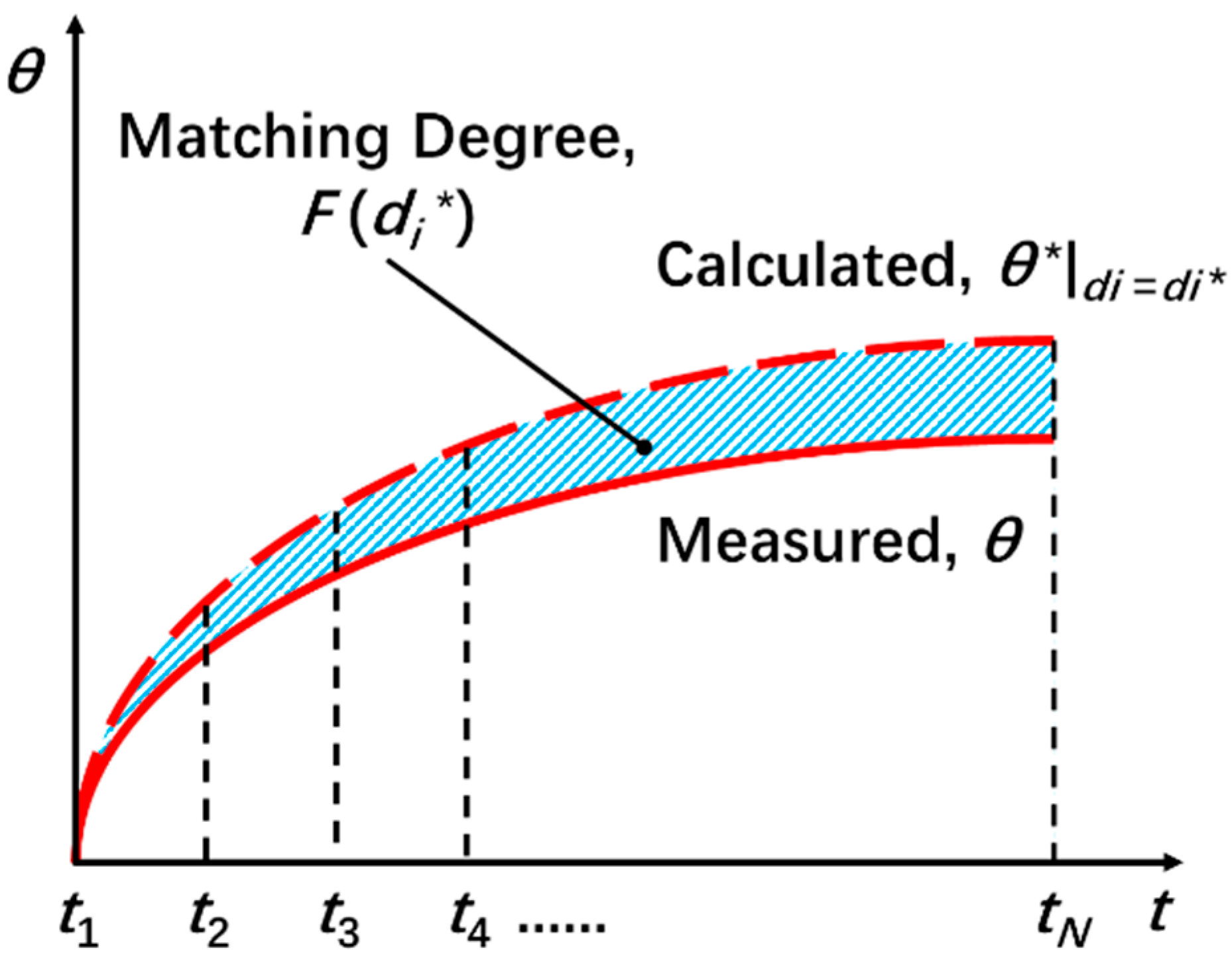
3. The Optimization Method Considering Thermal Boundary Conditions

Thermal boundary conditions are constant in a defined experimental environment, so the heat exchange time constant τ remains unchanged in the fatigue test [14,15,27]. Similarly, the material parameters ρ and C are also constant [14]. The left-hand side of Equation (4) can be thought of as an operator that represents the correspondence between temperature change θ and energy dissipation d_i. The constant parameters (ρ, C and τ) constrain the relationship represented by the operator. That is to say, the relationship between temperature change and energy dissipation is fixed.

Based on this invariant correspondence, we propose to adopt an optimization method for calculating energy dissipation directly from the thermal model representing temperature evolution under fatigue, as shown in Figure 1. First, the material parameters and the heat exchange constant in Equation (4) are set according to independent experiments. The operator representing the correspondence is then determined. Second, different values of energy dissipation rate are attempted to obtain a corresponding temperature evolution curve ${{\theta }^{*}|}_{d_i=d_i{}^{*}}$. At the same time, the degree of matching between each of the candidate temperature curves and the actual temperature measurement θ_measured is calculated separately based on a consistent criterion. At last, the trial temperature curve with the highest matching is found, and its corresponding energy dissipation is determined as the final result of the evaluation. In this way, the determination of energy dissipation is transformed into an optimization problem that seeks the minimum value of the matching function (objective function) with d_i as the independent variable. The final objective function F(d_i^*) for optimization is as shown in Equation (5).

$$F\left(d_i{}^{*}\right)=\sqrt{\frac{1}{t_n}{\displaystyle \sum }_0^{t_n}{\left[{\theta }_{measured}-{{\theta }^{*}|}_{d_i=d_i{}^{*}}\right]}^2}$$

(5)

where d_i^* is the energy dissipation rate tried during the optimization process, t_n is the length of the temperature data used to calculate the energy dissipation, and θ_measured is experimentally measured temperature data.

4. Numerical Simulation of Temperature Evolution during Fatigue

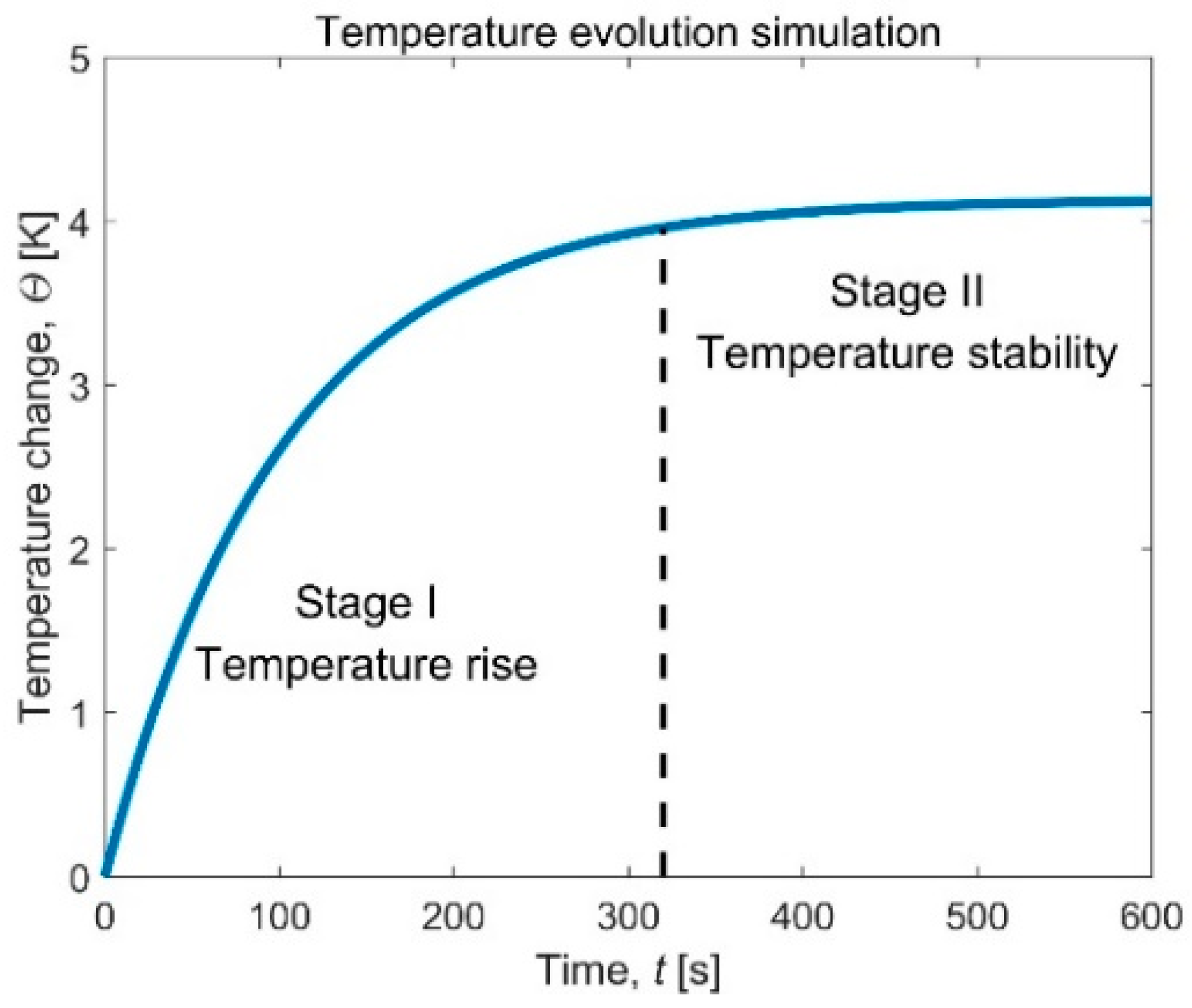
4.1. Temperature Evolution with Constant Energy Dissipation

Prepared for follow-up discussions, numerical simulation was performed to analyze the temperature evolution of the material under fatigue loading. The numerical simulation was conducted by using a self-programmed MATLAB code. Assuming a load frequency of 1 Hz, and the time step for simulation is set to 1 s. Since the time step is no longer than the cycle of the load, only the average temperature and energy dissipation rate for one load cycle are considered here, and temperature fluctuations caused by the thermoelastic effect are ignored [11,28]. The temperature evolution of the material was simulated by using the unit body thermal model shown in Equation (4). The material parameters in the thermal model were set according to A7N01 aluminum alloy, see

Table 1. Material parameters of A7N01.

Yield Strength, σs [MPa]	Density, ρ [kg/m3]	Heat Capacity, C [J/(kg·K)]	Thermal Conductivity, λ [W/(m·K)]
327	2690	900	119

. As confirmed by Zhang et al. [18], energy dissipation remains constant throughout the fatigue process when the load is consistent. Therefore, it can be assumed that the energy dissipation rate d_i = 1 × 10⁵ W/m³ under a certain stress level. The time constant τ represents the overall heat exchange condition determined by the experimental environment. Under a relatively stable experimental condition, the heat exchange time constant remains constant. In the analysis of this paper, τ will be set to different constants to show the influence of thermal boundary conditions on the temperature evolution of the specimen. As the first step, we first analyze the situation where τ is set to 100 s.

The temperature evolution of the numerical simulation is shown in Figure 2. It can be seen that the temperature evolution curve of the material during the fatigue process is divided into two stages. In Stage I, the heat generated by the energy dissipation in the material per unit time is greater than the heat lost to the surrounding environment, so that the temperature of the material rises rapidly [5]. As the temperature of the material increases, the temperature difference between the material and the environment becomes larger and larger. At the same time, the heat lost per unit time increases with the increase in the temperature difference. Until the heat loss rate is equal to the constant energy dissipation rate, the temperature of the material no longer rises, and the evolution curve enters Stage II with a steady-state temperature [15]. The simulated temperature profile follows a typical “two-stage” evolutionary trend, which is consistent with the experimental results in much of the literature [5,7,15,27]. This consistency ensures that the profile of the numerical simulation is consistent with the real temperature evolution of the material during fatigue before the occurrence of macroscopic cracks. It is reasonable to carry out further work based on these simulated temperature results.

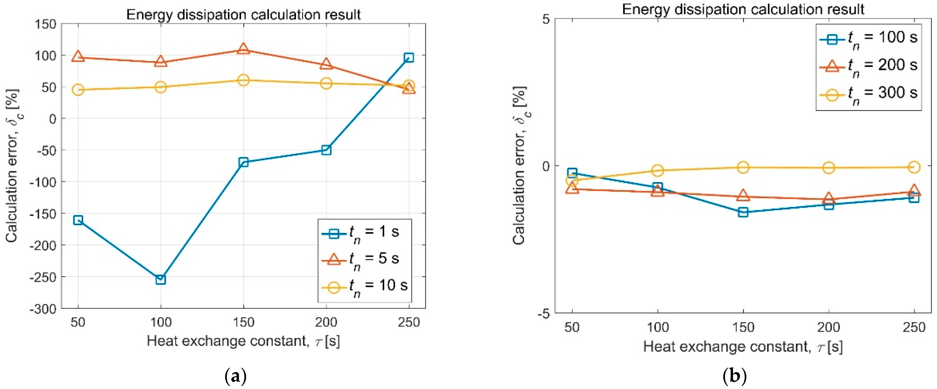
4.2. Influence of Thermal Boundary Conditions

The heat exchange conditions of the specimen in the fatigue test depend on the combination of many factors of the experimental environment, such as fatigue test equipment, ambient temperature, material and size of the specimen [10,14]. The experimental environment has a great influence on temperature, but it is difficult to be controlled by experimental means.

The time constant represents the overall heat exchange condition determined by the experimental environment. To analyze the effect of the experimental environment on temperature evolution during fatigue, the several heat exchange time constants τ with different values were, respectively, used to calculate the temperature evolution curve. The comparison of temperature evolution in different experimental environments is given in Figure 3 (the black dotted line). An array of random numbers uniformly distributed in the interval (−0.1, 0.1) is superimposed on the exact calculation result to simulate the real temperature measurement. Finally, the simulated temperature evolution fluctuates to a certain degree, as shown in Figure 3.

In general, each temperature profile has the same trend as in Figure 2. Discussion about the temperature evolution trend does not need to be repeated here. The temperature evolution curve with measurement noise is generally similar to the mere temperature calculation, but with significant irregular fluctuations.

Time constants with different values were utilized to indicate the effects of differences in the experimental environment. On the other hand, the other parameters of the thermal model remained fixed in each calculation. It means that the thermal boundary conditions determined by the experimental environment are the only variables. The simulation results for different time constants correspond to the experiments performed in different environments, with the same material (same material parameters) and the same load (same energy dissipation). With an increased time constant τ, the material has a greater degree of temperature rise during the temperature stabilization stage. It is because the larger time constant τ, the harder it is to lose the heat in the fatigue specimen into the surrounding environment. A steady temperature means that the slope of the temperature evolution curve is zero.

$$\frac{d\theta }{dt}=0$$

(6)

Equation (6) is brought into Equation (4), resulting in

$${\theta }_{steady}=\frac{d_i}{\rho C}\tau$$

(7)

where θ_steady is the temperature rise in the steady stage. Energy dissipation d_i, density ρ and specific heat C are consistent for different temperature curves. Therefore, according to Equation (7), the steady-state temperature θ_steady will linearly increase along with the heat exchange time constant τ.

5. Validation of the Optimization Method Based on Numerical Simulation

In this section, the effectiveness of the optimization method will be verified, in which the results of the numerical simulation are used in preference to the actual temperature measurement. The advantage of this is that it is easy to figure out whether the optimization method makes an accurate assessment of the energy dissipation by comparing the results calculated from the temperature data with the preset accurate values.

5.1. Result of the Optimization Method

Taking the simulation results as known temperature information, the energy dissipation was calculated by the optimization method. The material parameters and the heat exchange time constant were also known conditions in energy dissipation evaluation since they can be determined in advance by independent testing. The calculation error δ_c of the method with respect to the exact value was evaluated according to Equation (8).

$${\delta }_c=\frac{d_{evaluated}-d_{exact}}{d_{exact}}\times 100\%$$

(8)

where d_evaluated is the evaluation result of energy dissipation, and d_exact is the exact value previously set (1 × 10⁵ W/m³).

Figure 4 shows the energy dissipation calculation by the optimization method based on different length (t_n) of temperature measurement simulations. When t_n is small (t_n = 1, 5, 10 s), the result of the calculation is highly unstable, which is the case as shown in Figure 4a. A smaller t_n means that only limited temperature data is utilized for the calculation of energy dissipation. Slight fluctuations caused by measurement noise will lead to sharp oscillations in the final result. When t_n is big enough (t_n = 100, 200, 300 s), the calculation error between the result of the optimization method and the exact value is all less than ±3%, as shown in Figure 4b. More temperature data can be used to calculate energy dissipation as t_n increases. This means that more effective information can be used. In contrast, the magnitude of the measurement noise is permanent, which depends on the measurement approach. Random measurement noise cancels each other during the calculation. When t_n is greater than a certain degree, the estimation of the energy dissipation tends to be stable and accurate with the elimination of the influence of the measurement noise, as shown in Figure 5.

It can be found that using more temperature data is beneficial to obtain better results for the optimization method. This feature of the optimization method helps to ensure the accuracy of its calculation of energy dissipation, because more temperature data can be obtained by simply increasing the time of measuring the temperature.

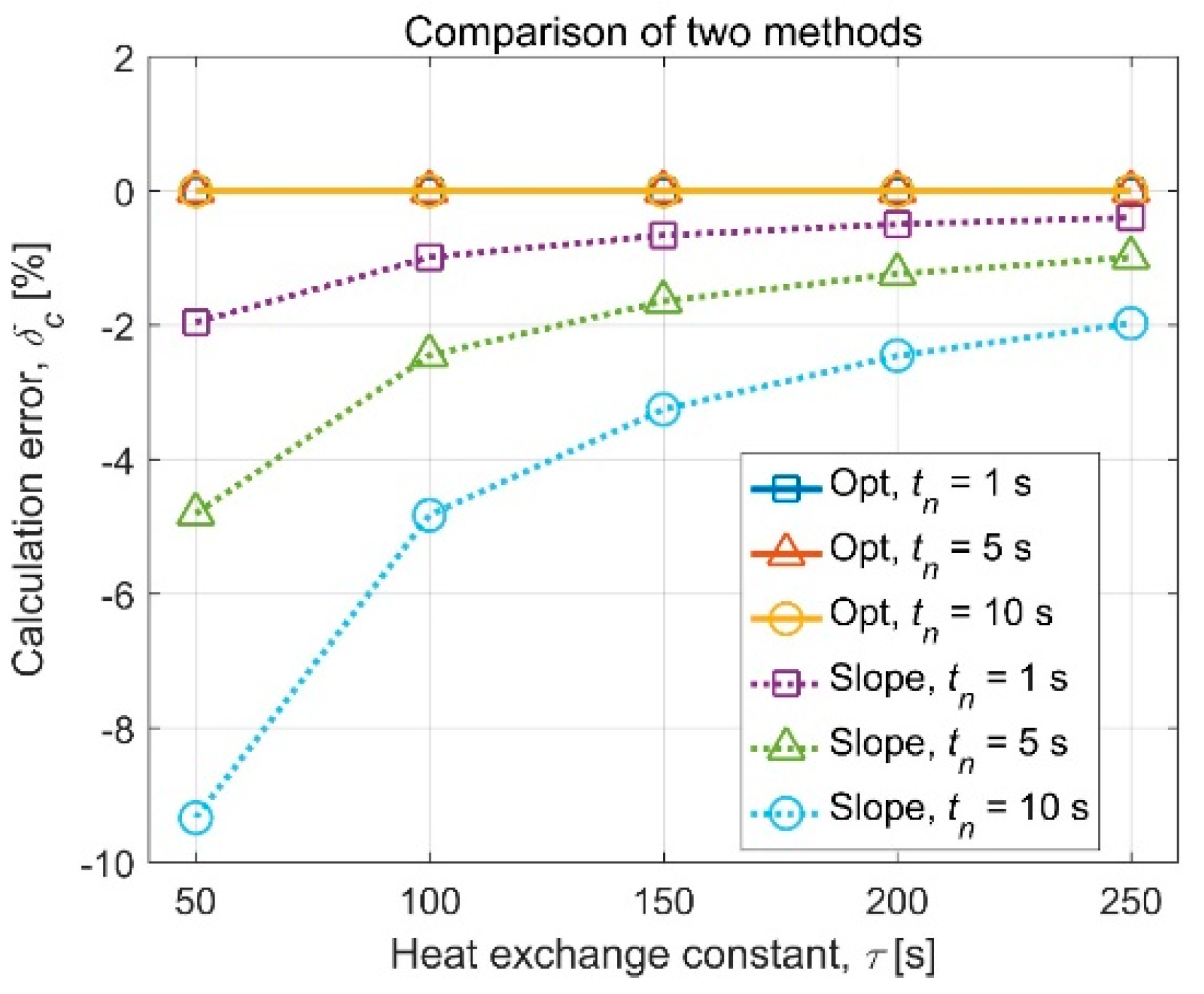
5.2. Comparison with the Slope Method

For comparison in the subsequent sections of this paper, we need to review the popular slope method [18,20]. The experimental environment can be considered as adiabatic at the very beginning of the fatigue loading, because the time is too short to allow the specimen to exchange heat with the external environment [16]. The second term on the left-hand side of in Equation (4) that represents all the heat loss can be ignored, and we receive a special form of the thermal model that only holds when t equals zero.

$$\rho C{\frac{d\theta }{dt}|}_{t=0}=d_i$$

(9)

According to the customary nomenclature, let

$$R_{\theta }={\frac{d\theta }{dt}|}_{t=0}$$

(10)

The energy dissipation under fatigue can be calculated based on the initial slope of the temperature evolution curve R_θ, as shown in Figure 6, which is the so-called slope method.

$$d_i=\rho C{R}_{\theta }$$

(11)

The actual temperature data is discrete and not smooth due to the thermoelastic effect and the measurement noise. In practice, a linear fit through a certain length [0, t_n] of the recorded temperature data is utilized to determine R_θ, as shown in Figure 7 [19]. To satisfy the premise of Equation (9) that t = 0, a small t_n is usually taken [20].

It can be easily seen from the principle that the most essential difference between the optimization method and the slope method lies in the treatment of thermal boundary conditions. In the optimization method, the actual measured thermal boundary conditions are used. In the slope method, the thermal boundary conditions are assumed to be adiabatic. Therefore, the accuracy of the slope method is largely restricted by the rationality of the adiabatic assumption. Only under adiabatic conditions, all energy dissipation is utilized to increase the temperature of the material. In this case, the assessment of the slope method for energy dissipation is accurate. It requires the time constant τ to be infinite [29]. However, the actual experiment cannot be an ideal adiabatic situation, and the specimen inevitably exchanges heat with the outside world. It means that τ must be finite. The larger time constant makes the thermal boundary conditions closer to adiabatic, and the slope method results are more accurate. Figure 8 shows the calculation results of the slope method for energy dissipation under different thermal boundary conditions. As mentioned before, the time constant τ characterizes the ability of the material to exchange heat with the external environment. The larger the τ, the harder it is to lose heat. As shown in Figure 8, the result of a larger heat exchange time constant τ is better than that of a smaller one.

On the other hand, it can be found from Figure 8 that the smaller the t_n, the more accurate the results of the slope method. This trend results from the requirement of the slope method for t_n to approach zero [30]. A larger t_n means that there is more time for the heat in the material to escape into the external environment and more heat to be lost. In this case, the amount of heat lost is considerable, and the effects of heat loss should not be ignored. The heat loss causes a decrease in the temperature rise rate of the material, which is reflected as a decrease in the slope of the temperature evolution curve. However, the slope method still approximates the rise in material temperature as a result of energy dissipation only and converts the lost heat into the final result. Therefore, the calculation of energy dissipation continuously underestimated as t_n increases.

As a comparison, the results of the optimization method are all in good agreement with the preset exact value. In any case, the optimization method has better calculation results than the slope method. The optimization method performs well in different τ, indicating that it is an energy dissipation evaluation method that is not affected by the experimental environment. Moreover, unlike that the t_n must be quite limited in the slope method, the optimization method has flexible requirements for the length of the temperature data used for calculation.

The fundamental advantage of the optimization method over the slope method is the direct use of the thermal boundary conditions obtained through experimental measurements. Less simplification leads to more accurate final assessment results. The key to accurate energy dissipation assessment by the slope method is to minimize heat loss to the outside world. However, in actual experiments, there is always some heat lost, which makes the evaluation of the slope method approximate.

6. Application: Fatigue Life Analysis

It has been proved that the optimization method is an effective energy dissipation evaluation approach, which is competent for the actual situation that contains measurement noise. In this section, the optimization method was applied to evaluate the energy dissipation of the A7N01 and its butt joints under high cycle fatigue loads. Subsequently, a fatigue life model based on the above energy dissipation assessment was established and compared with the traditional S-N model.

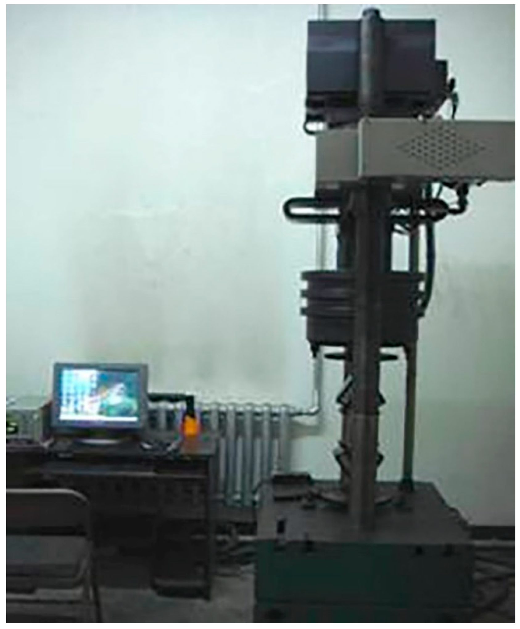
6.1. Experimental Materials and Procedures

A7N01 is a kind of aluminum alloy used in the main structure of high-speed trains, whose material parameters are shown in Table 1. The butt joint was prepared by manual gas tungsten arc welding (GTAW) using a 6 mm thick A7N01 plate, and the filler material was selected to be ER5356 with a diameter of 1.6 mm (produced by SAF-PRO). The welding process was conducted according to the following parameters: current 200 A, voltage 23–25 V, welding speed 1.67 mm/s, and gas flow 15 L/min. The chemical compositions of A7N01 and ER5356 are given in

Table 2. Chemical compositions of A7N01 alloy and wires ER5356 (wt.%).

Materials	Si	Fe	Cu	Mu	Mg	Cr	Zn	Ti	Al
A7N01	0.35	0.40	0.20	0.15	1.20	0.20	4.60	-	Bal.
ER5356	0.057	0.12	0.011	<0.13	4.9	0.065	0.13	0.11	Bal.

. The yield strength of the A7N01 and the joints was previously tested by static tensile testing, 327 MPa and 238 MPa, respectively.

The stress-controlled fatigue test was carried out using a PLG-100C electromagnetic resonance fatigue machine, as shown in Figure 9. A uniaxial sinusoidal load with a constant stress amplitude was used for the test. The load frequency is 128 Hz, and the stress ratio is R = 0 (the ratio of the minimum stress to the maximum stress). The stress level is set to be less than the yield strength (140, 150, 160, 170 MPa for the base and 130, 140, 150, 160 MPa for the welded joints). The dimensions of the fatigue specimen are given in Figure 10. Fatigue cracks will lead to a reduction in load frequency and load stress. When any of the load frequency and the load stress is reduced by 10%, the fatigue test is terminated due to the automatic protection of the testing machine, and it is considered that fatigue failure has occurred.

Temperature measurements on the center of the specimen were performed using a self-designed temperature measurement system during the fatigue test. The measurement system has an accuracy of ±0.1 °C and a sampling frequency of 2 Hz. More details about the temperature measurement system can be found in Reference [18]. The temperature sensor is firmly fixed to the surface of the specimen. In addition, insulation measures are applied to impede the loss of heat through the convection and the heat transfer between the specimen and the clamp of fatigue tester. Based on the measured temperature data, the optimization process for calculating the energy dissipation is performed using the MATLAB program in an automated way.

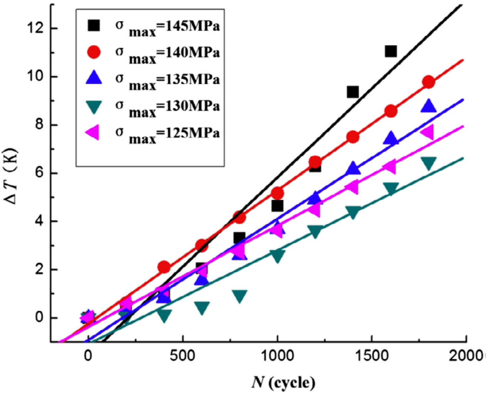
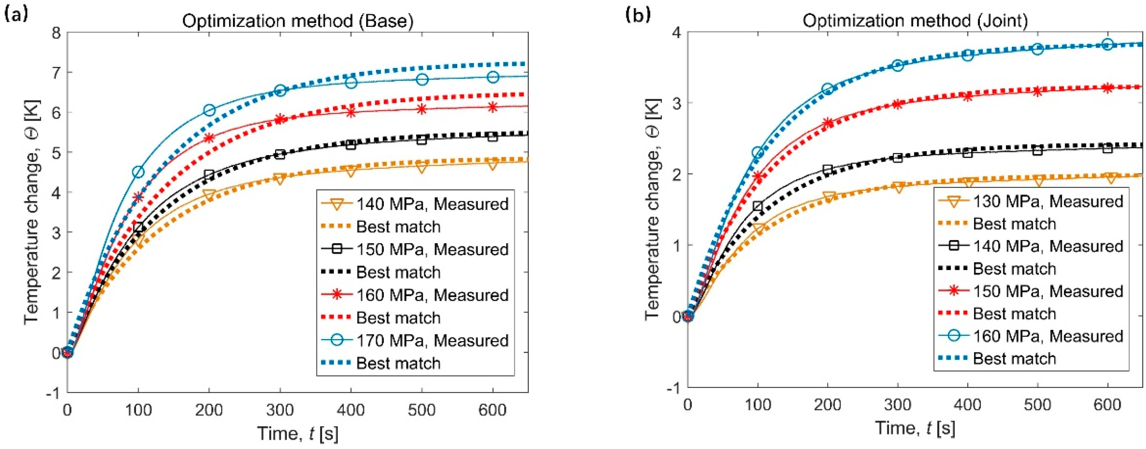
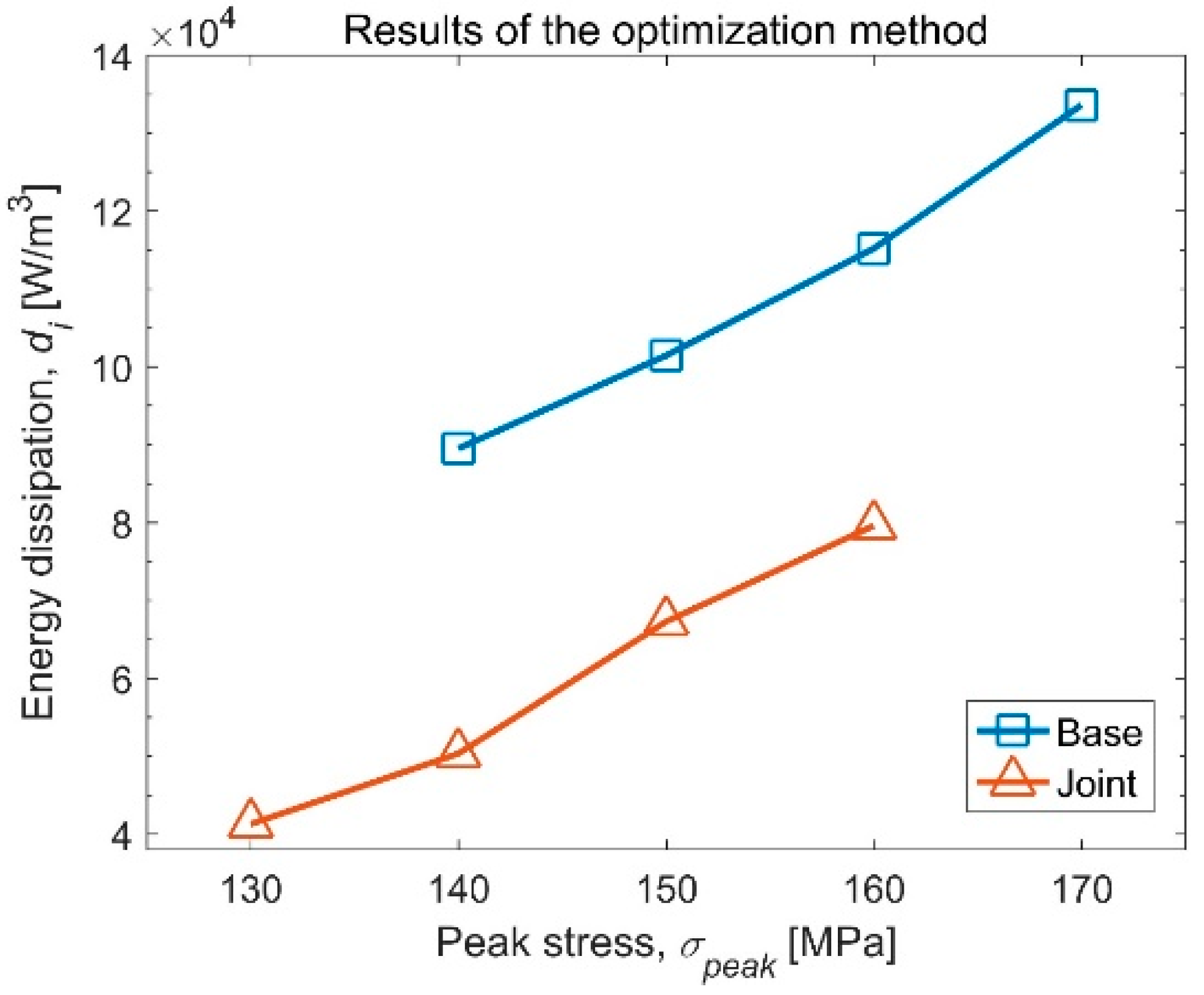
6.2. Results and Discussion

Figure 11 represents a measurement of the temperature evolution of A7N01 aluminum alloy and its welded joints under high cycle fatigue. θ is the temperature change at the center of the specimen, which is equal to the difference between the center temperature T of the test piece and the initial temperature T₀, θ = T − T₀. Since the sampling rate of the temperature measuring device is much smaller than the frequency of the load, temperature fluctuations caused by the thermoelastic effect cannot be faithfully recorded. It is more appropriate to consider the results in Figure 11 as the average temperature of multiple load cycles. Ignoring these thermoelastic temperature fluctuations does not interfere with the calculation of energy dissipation because the effect of energy dissipation is mainly reflected in the change of the average temperature [31,32]. After a period of temperature rise, each temperature evolution curve gradually enters a relatively stable stage. It means that, in the fatigue test, the heat loss from the A7N01 aluminum alloy and its joint to the outside finally reaches the dynamic balance with the internal heat generation (energy dissipation).

Next, the newly proposed optimization method is employed to calculate the energy dissipation based on the temperature data in Figure 11. According to previous numerical simulation experiments, the use of more temperature data helps to overcome the effects of measurement noise and obtain a better evaluation of energy dissipation. Here, we extend the length of the temperature data used for calculation t_n to 600 s to ensure that the evaluation of energy dissipation is accurate. The heat exchange time constant is determined in advance by an independent test. τ = 131.6 s for the A7N01 base specimen and τ = 116.4 s the butt joint specimen. The best matching curve is displayed by the dotted line in Figure 11, and the corresponding energy dissipation calculation result is given in Figure 12. It is clear that the energy dissipation per unit time goes up with the increasing load levels, which is true for A7N01 aluminum alloys and their welded joints. This relationship between the energy dissipation rate and the applied load in this work follows the general rule found in many existing studies. A detailed explanation can be found in Reference [11], and only a brief description is given here. In general, the majority of the mechanical work used to cause microscopic plastic deformation is converted into heat. Higher applied loads result in greater amount of plastic deformation. More mechanical work is converted into heat in unit time. These heats converted from mechanical work are energy dissipation. Therefore, the higher the load level, the greater the energy dissipation rate. In addition, the larger energy dissipation rate caused by the higher stress level is also intuitively reflected in the higher stable temperature θ_steady. Once more, a description of the specimen temperature in the equilibrium stage, Equation (7), is quoted. For tests at different stress levels, the heat exchange time constant τ is consistent because the experimental conditions affecting heat loss are the same. The same experimental material maintains that the material parameters ρ and C are also constant. It is obvious that the steady temperature θ_steady will increase as the energy dissipation d_i increases.

Many investigations have reported that the energy dissipation is intimately related to fatigue performance [33]. Among them, the limit energy model is a widely accepted one. The limit energy model believes that the total amount of energy dissipation before fatigue failure is a constant for the same material under different stress levels [18,32,34], as shown in Equation (12).

$$\mathsf{\Phi }=\underset{0}{\overset{N_f}{{\displaystyle \int }}}\frac{d_i}{f_n}dN=constant$$

(12)

where d_i is the energy dissipation per unit time, f_n is the load frequency, N_f is the fatigue life, and Φ is the total amount of energy dissipation before fatigue failure. If the load is constant, the energy dissipation of the material will not change over time [18,31]. Equation (12) can be written as follows:

$$N_f·\frac{d_i}{f_n}=\mathsf{\Phi }$$

(13)

The limit energy model illustrates the relationship between energy dissipation and fatigue life. In the previous studies, it has been confirmed that Equation (13) has the ability to predict fatigue life for various metals [18,19,31]. This time, the optimization method replaces the conventional slope method, and its energy dissipation evaluation results were used to analyze the fatigue life according to the limit energy model. The Φ value was derived from the average value of Φ_i that was calculated according to Equation (13) at different stress levels. The value of Φ is 4.12 × 10⁸ and 2.79 × 10⁸ J/m³ for A7N01 base and the welded joints, respectively. Figure 13a shows the experimental results and predicted fatigue life by the limit energy model.

Table 3. Comparison between results of fatigue test and the limit energy model (A7N01 base).

σpeak (MPa)	di (W/m3)	Nexp	Φi (J/m3)	Φ (J/m3)	Npre	δp (%)
140	8.95 × 104	582,528	4.07 × 108	4.12 × 108	589,791	1.25
150	1.01 × 105	499,585	3.96 × 108		520,401	4.17
160	1.15 × 105	501,696	4.51 × 108		458,319	−8.65
170	1.34 × 105	378,432	3.95 × 108		395,158	4.42

and

Table 4. Comparison between results of fatigue test and the limit energy model (Welded joints).

σpeak (MPa)	di (W/m3)	Nexp	Φi (J/m3)	Φ (J/m3)	Npre	δp (%)
130	4.13 × 104	1,358,528	4.38 × 108	2.79 × 108	866,184	−36.24
140	5.03 × 104	626,177	2.46 × 108	-	710,410	13.45
150	6.73 × 104	457,023	2.40 × 108	-	531,458	16.29
160	7.96 × 104	310,080	1.93 × 108	-	449,247	44.88

exhibit the comparison between the experimental fatigue life and the theoretical model life at different peak stress σ_peak. The prediction error δ_p could be defined as,

$${\delta }_p=\frac{N_{pre}-N_{exp}}{N_{exp}}\times 100\%$$

(14)

where N_exp means the experimental life and N_pre means the predicted life estimated by the energy model. Meanwhile, the prediction results of the traditional S-N model are also given in Figure 13b.

As shown in Table 3, the prediction error of the limit energy model is less than 10% at all given stress levels, which is a satisfactory prediction for high cycle fatigue. It should be noted that all the given stress levels belong to the range of short fatigue life. The effectiveness of the new method for long fatigue life needs further experimental verification. The author will carry out this work in the future. It is also worth noting that the limit energy model has only one parameter, Φ, but the S-N model has two parameters [35]. In general, theoretical models with more parameters should have a better description of the experimental data. However, the limit energy model provides better predictions with fewer model parameters. In Figure 14a, the limit energy model predicts fatigue life better than the traditional S-N model under three of all four stress levels. Additionally, the average value of |δ_p| (absolute value of prediction error) of the limit energy model is 4.62%, while that of the S-N model is 5.82%. It may mean that the energy dissipation-based fatigue model is more in line with the physical nature of fatigue than statistical models. For practical applications, models with fewer parameters require less experimental data and are more economical. Fatigue studies based on energy dissipation are of potential, but more research is needed to finally confirm the advantages of the limit energy model.

For the butt joint of the A7N01, neither model gives the same accurate prediction results as the base metal. The prediction error of the energy model is up to 44.88%, as shown in Table 4, and the prediction error of the traditional S-N model is also over 30%. The reason may be that the joint inevitably contains some defects caused by the welding process, thus the dispersion of the fatigue properties of the joint is inherently greater than that of the base metal [18]. Comparing the two models, the limit energy model predicts the fatigue life of the joints worse than the S-N model, as shown in Figure 14b, which is different from the case of A7N01 base. The zero-dimensional heat conduction model used in this paper is based on the assumption of uniform internal heat source distribution. The non-uniformity of the welding seam causes uneven internal heat source distribution. To a certain extent, this affects the calculation of energy dissipation at the local location where fatigue damage occurs in the joint specimen [9,14]. A more complex temperature model is needed to cope with the unevenness of the welded joint.

7. Conclusions

Within the framework of the zero-dimensional thermal diffusion model, this paper presents a calculation method for evaluating the energy dissipation of materials in the initial stage of fatigue, which can be called the optimization method. Different from the popular slope method, this method takes the influence of thermal boundary conditions into consideration. Numerical simulation showed that the optimization method has the ability to accurately estimate energy dissipation in different experimental environments and is not sensitive to measurement noise. Compared with the popular slope method, the newly proposed optimization method has certain advantages in adaptability to different environments and flexibility in parameter selection. A case study was also carried out to study a high-cycle fatigue life of an aluminum alloy which demonstrated that results predicted by the proposed method matched the experimental data in the range of short fatigue life.

References

1. Khonsari, M.M.; Amiri, M. Introduction to Thermodynamics of Mechanical Fatigue; CRC Press: New York, NY, USA, 2013. [Google Scholar]
2. Connesson, N.; Maquin, F.; Pierron, F. Dissipated Energy Measurements as a Marker of Microstructural Evolution: 316L and DP600. Acta Mater. 2011, 59, 4100–4115. [Google Scholar] [CrossRef]
3. Zhang, H.X.; Wu, G.H.; Yan, Z.F.; Guo, S.F.; Chen, P.D.; Wang, W.X. An Experimental Analysis of Fatigue Behavior of AZ31B Magnesium Alloy Welded Joint Based on Infrared Thermography. Mater. Des. 2014, 55, 785–791. [Google Scholar] [CrossRef]
4. Crupi, V. An Unifying Approach to Assess the Structural Strength. Int. J. Fatigue 2008, 30, 1150–1159. [Google Scholar] [CrossRef]
5. Luong, M.P. Fatigue Limit Evaluation of Metals Using an Infrared Thermographic Technique. Mech. Mater. 1998, 28, 155–163. [Google Scholar] [CrossRef]
6. La Rosa, G.; Risitano, A. Thermographic Methodology for Rapid Determination of the Fatigue Limit of Materials and Mechanical Components. Int. J. Fatigue 2000, 22, 65–73. [Google Scholar] [CrossRef]
7. Fargione, G.; Geraci, A.; La Rosa, G.; Risitano, A. Rapid Determination of the Fatigue Curve by the Thermographic Method. Int. J. Fatigue 2002, 24, 11–19. [Google Scholar] [CrossRef]
8. Bouache, T.; Pron, H.; Caron, D. Identification of the Heat Losses at the Jaws of a Tensile Testing Machine. Exp. Mech. 2016, 56, 287–295. [Google Scholar] [CrossRef]
9. Facchinetti, M.; Florin, P.; Doudard, C.; Calloch, S. Identification of Self-Heating Phenomena under Cyclic Loadings Using Full-Field Thermal and Kinematic Measurements: Application to High-Cycle Fatigue of Seam Weld Joints. Exp. Mech. 2015, 55, 681–698. [Google Scholar] [CrossRef]
10. Chrysochoos, A.; Louche, H. An Infrared Image Processing to Analyse the Calorific Effects Accompanying Strain Localisation. Int. J. Eng. Sci. 2000, 38, 1759–1788. [Google Scholar] [CrossRef]
11. Guo, S.; Zhou, Y.; Zhang, H.; Yan, Z.; Wang, W.; Sun, K.; Li, Y. Thermographic Analysis of the Fatigue Heating Process for AZ31B Magnesium Alloy. Mater. Des. 2015, 65, 1172–1180. [Google Scholar] [CrossRef]
12. Guo, Q.; Guo, X.; Fan, J.; Syed, R.; Wu, C. An Energy Method for Rapid Evaluation of High-Cycle Fatigue Parameters Based on Intrinsic Dissipation. Int. J. Fatigue 2015, 80, 136–144. [Google Scholar] [CrossRef]
13. Guo, Q.; Guo, X. Research on High-Cycle Fatigue Behavior of FV520B Stainless Steel Based on Intrinsic Dissipation. Mater. Des. 2016, 90, 248–255. [Google Scholar] [CrossRef]
14. Boulanger, T.; Chrysochoos, A.; Mabru, C.; Galtier, A. Calorimetric Analysis of Dissipative and Thermoelastic Effects Associated with the Fatigue Behavior of Steels. Int. J. Fatigue 2004, 26, 221–229. [Google Scholar] [CrossRef]
15. Meneghetti, G. Analysis of the Fatigue Strength of a Stainless Steel Based on the Energy Dissipation. Int. J. Fatigue 2007, 29, 81–94. [Google Scholar] [CrossRef]
16. Amiri, M.; Khonsari, M.M. Rapid Determination of Fatigue Failure Based on Temperature Evolution: Fully Reversed Bending Load. Int. J. Fatigue 2010, 32, 382–389. [Google Scholar] [CrossRef]
17. Amiri, M.; Khonsari, M.M. Life Prediction of Metals Undergoing Fatigue Load Based on Temperature Evolution. Mater. Sci. Eng. A 2010, 527, 1555–1559. [Google Scholar] [CrossRef]
18. Zhang, L.; Liu, X.S.; Wu, S.H.; Ma, Z.Q.; Fang, H.Y. Rapid Determination of Fatigue Life Based on Temperature Evolution. Int. J. Fatigue 2013, 54, 1–6. [Google Scholar] [CrossRef]
19. Liu, X.Q.; Zhang, H.X.; Yan, Z.F.; Wang, W.X.; Zhou, Y.G.; Zhang, Q.M. Fatigue Life Prediction of AZ31B Magnesium Alloy and its Welding Joint through Infrared Thermography. Theor. Appl. Fract. Mech. 2013, 67–68, 46–52. [Google Scholar]
20. Amiri, M.; Khonsari, M.M. Nondestructive Estimation of Remaining Fatigue Life: Thermography Technique. J. Fail. Anal. Prev. 2012, 12, 683–688. [Google Scholar] [CrossRef]
21. Liakat, M.; Naderi, M.; Khonsari, M.M.; Kabir, O.M. Nondestructive Testing and Prediction of Remaining Fatigue Life of Metals. J. Nondestruct. Eval. 2014, 33, 309–316. [Google Scholar] [CrossRef]
22. Liakat, M.; Khonsari, M.M. An Experimental Approach to Estimate Damage and Remaining Life of Metals under Uniaxial Fatigue Loading. Mater. Des. 2014, 57, 289–297. [Google Scholar] [CrossRef]
23. Williams, P.; Liakat, M.; Khonsari, M.M.; Kabir, O.M. A Thermographic Method for Remaining Fatigue Life Prediction of Welded Joints. Mater. Des. 2013, 51, 916–923. [Google Scholar] [CrossRef] [Green Version]
24. Haghshenas, A.; Khonsari, M.M. Non-Destructive Testing and Fatigue Life Prediction at Different Environmental Temperatures. Infrared Phys. Technol. 2019, 96, 291–297. [Google Scholar] [CrossRef]
25. Mehdizadeh, M.; Khonsari, M.M. On the Application of Fracture Fatigue Entropy to Variable Frequency and Loading Amplitude. Theor. Appl. Fract. Mech. 2018, 98, 30–37. [Google Scholar] [CrossRef]
26. Mehdizadeh, M.; Khonsari, M.M. On the Role of Internal Friction in Low-And High-Cycle Fatigue. Int. J. Fatigue 2018, 114, 159–166. [Google Scholar] [CrossRef]
27. Mareau, C.; Favier, V.; Weber, B.; Galtier, A. Influence of the Free Surface and the Mean Stress on the Heat Dissipation in Steels under cyclic loading. Int. J. Fatigue 2009, 31, 1407–1412. [Google Scholar] [CrossRef]
28. Wang, X.G.; Feng, E.S.; Jiang, C. A Microplasticity Evaluation Method in Very High Cycle Fatigue. Int. J. Fatigue 2017, 94, 6–15. [Google Scholar] [CrossRef] [Green Version]
29. Delpueyo, D.; Balandraud, X.; Grédiac, M.; Stanciu, S.; Cimpoesu, N. A Specific Device for Enhanced Measurement of Mechanical Dissipation in Specimens Subjected to Long-Term Tensile Tests in Fatigue. Strain 2018, 54, e12252. [Google Scholar] [CrossRef]
30. De Finis, R.; Palumbo, D.; Da Silva, M.M.; Galietti, U. Is the Temperature Plateau of a Self-Heating Test a Robust Parameter to Investigate the Fatigue Limit of Steels with Thermography? Fatigue Fract. Eng. Mater. Struct. 2018, 41, 917–934. [Google Scholar] [CrossRef]
31. Fan, J.; Guo, X.; Wu, C. A New Application of the Infrared Thermography for Fatigue Evaluation and Damage Assessment. Int. J. Fatigue 2012, 44, 1–7. [Google Scholar] [CrossRef]
32. Fan, J.; Zhao, Y.; Guo, X. A Unifying Energy Approach for High Cycle Fatigue Behavior Evaluation. Mech. Mater. 2018, 120, 15–25. [Google Scholar] [CrossRef]
33. Guo, Q.; Zaïri, F.; Guo, X. An Intrinsic Dissipation Model for High-Cycle Fatigue Life Prediction. Int. J. Mech. Sci. 2018, 140, 163–171. [Google Scholar] [CrossRef]
34. Fan, J.L.; Guo, X.L.; Wu, C.W.; Zhao, Y.G. Research on Fatigue Behavior Evaluation and Fatigue Fracture Mechanisms of Cruciform Welded Joints. Mater. Sci. Eng. A 2011, 528, 8417–8427. [Google Scholar] [CrossRef]
35. Suresh, S. Fatigue of Materials; Cambridge University Press: Cambridge, UK, 1998. [Google Scholar]
Figure 1. Schematic diagram of the optimization method.
Metals 11 01512 g001
Figure 2. Numerical simulation of temperature evolution during fatigue.
Metals 11 01512 g002
Figure 3. Comparison of temperature evolution with different time constants τ.
Metals 11 01512 g003
Figure 4. Calculation result of the optimization method: (a) tn = 1, 5, 10 s; (b) tn = 100, 200, 300 s.
Metals 11 01512 g004
Figure 5. Calculation of energy dissipation based on temperature measurement with varied lengths tn using optimization method (τ = 100 s).
Metals 11 01512 g005
Figure 6. Schematic diagram of the slope method.
Metals 11 01512 g006
Figure 7. Linear fit for calculating Rθ in the slope method [19].
Metals 11 01512 g007
Figure 8. Comparison of energy dissipation calculation between the optimization method and the slope method (without measurement noise).
Metals 11 01512 g008
Figure 9. PLG-100C electromagnetic resonance fatigue machine.
Metals 11 01512 g009
Figure 10. Dimensions of the fatigue specimen.
Metals 11 01512 g010
Figure 11. Temperature evolution of (a) A7N01 aluminum alloy and (b) its welded joints under high cycle fatigue.
Metals 11 01512 g011
Figure 12. Evaluation results of the optimization method for actual experiments.
Metals 11 01512 g012
Figure 13. Experimental fatigue life and prediction of theoretical models: (a) the limit energy model; (b) the S-N model.
Metals 11 01512 g013
Figure 14. Comparison of two life prediction models: (a) base metal; (b) welded joint.
Metals 11 01512 g014