
High-Entropy Alloys Properties Prediction Model by Using Artificial Neural Network Algorithm


Abstract
:1. Introduction
2. Methodology
2.1. HEAs Data Information
2.2. Data Preprocessing and Model Evaluation
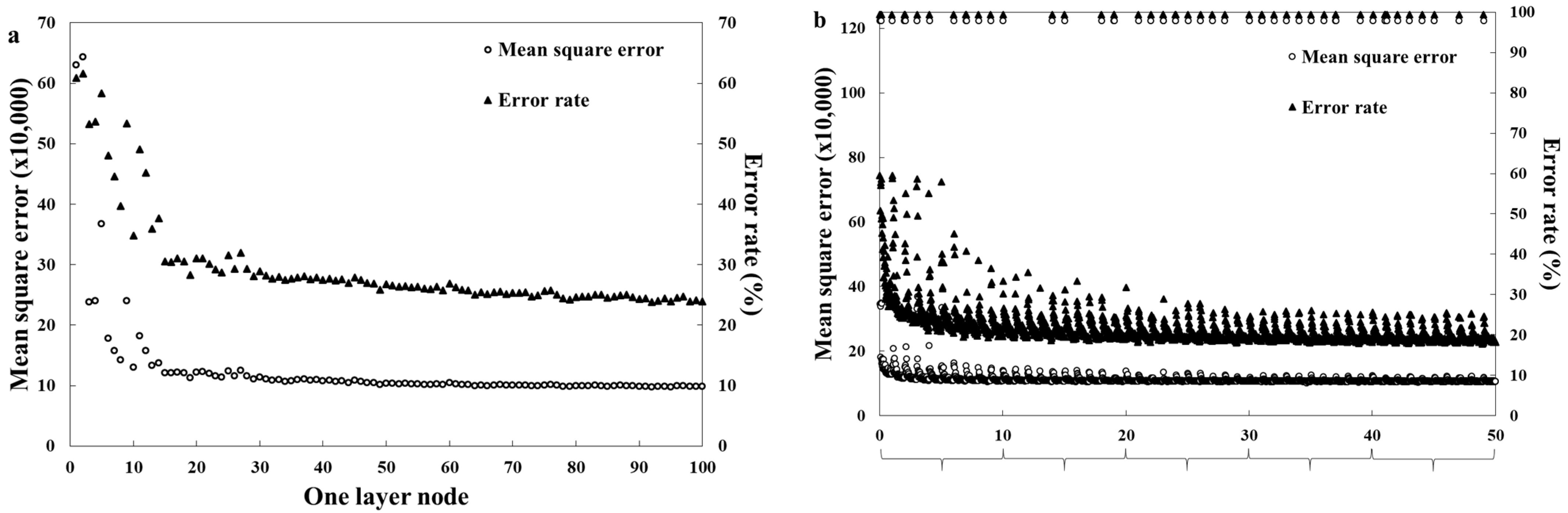
Optimization Process for ANN Prediction Model
2.3. Optimization Process for Lasso Linear Regression Prediction Model
3. Results and Discussion
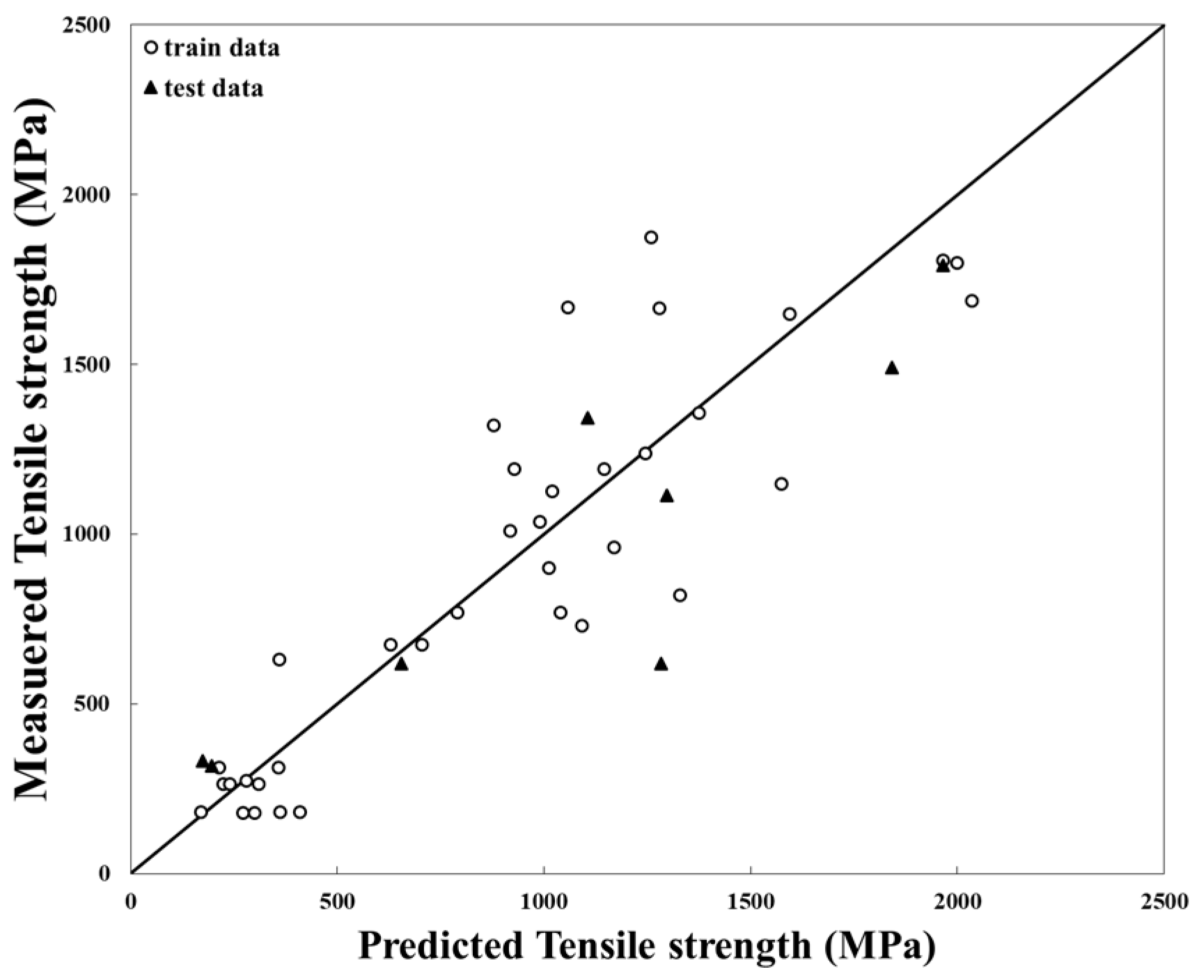
3.1. Evaluation Predicting Accuracy of ANN Models
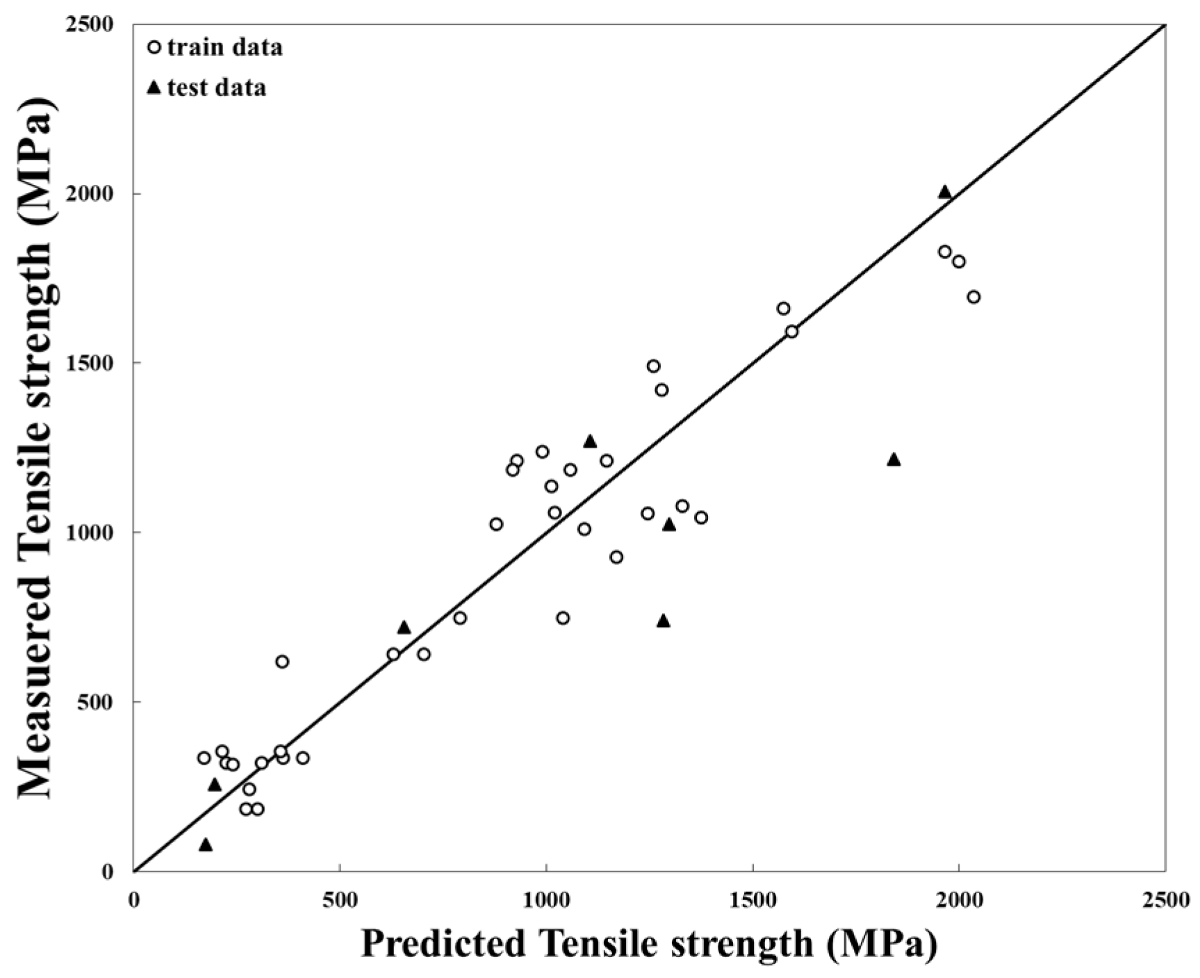
3.2. Evaluation Predicting Accuracy of Lasso Linear Models
3.3. Effect of Process Input Data on Transition Metals and Refractory Metals
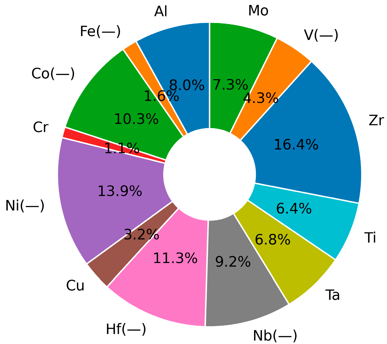
3.4. Assessment of the Influence of Elements in Alloys
4. Conclusions
- The ANN prediction model showed high accuracy only when learning the post-process data together; the tensile strength showed an error rate of 19.7%, and the microstructure was consistent in all test data. Elongation prediction showed a high error rate of 40.2%.
- In the case of the lasso linear regression, the error rate of the model trained with post-processing data was 31.1%, and the error rate of the lasso model trained only on the mole fraction was 26.1%, showing low accuracy. The linear regression model did not sufficiently reflect the complex causal relationships in the data as the variable increased.
- When post-process data were trained with the element mole fraction, the model error rate decreased from 15.9% to 14% in the refractory metal group, and the error rate of the transition metal group decreased from 52% to 27% in the transition metal group. In contrast, the lasso model showed the opposite trend.
- In the ANN model, Al, Cr, Cu, Nb, Ta, Ti, Zr, Mo, and W increased the strength as these components increased, and Co, Fe, Ni, Mn, Hf, and V decreased the tensile strength. In the lasso model, the same results were obtained except for Nb. In addition, in the post-process, cold rolling and forging improved the tensile strength.
Author Contributions
Funding
Institutional Review Board Statement
Informed Consent Statement
Data Availability Statement
Acknowledgments
Conflicts of Interest
References
- Yeh, J.W. Alloy design strategies and future trends in high-entropy alloys. JOM 2013, 65, 1759–1771. [Google Scholar] [CrossRef]
- Singh, S.; Wanderka, N.; Kiefer, K.; Siemensmeyer, K.; Banhart, J. Effect of decomposition of the Cr-Fe-Co rich phase of AlCoCrCuFeNi high entropy alloy on magnetic properties. Ultramicroscopy 2011, 111, 619–622. [Google Scholar] [CrossRef]
- Gao, M.C.; Zhang, B.; Guo, S.M.; Qiao, J.W.; Hawk, J.A. High-entropy alloys in hexagonal close-packed structure. Metall. Mater. Trans. A 2016, 47, 3322–3332. [Google Scholar] [CrossRef]
- Zhang, C.; Zhang, F.; Chen, S.; Cao, W. Computational thermo.dynamics aided high-entropy alloy design. JOM 2012, 64, 839–845. [Google Scholar] [CrossRef]
- Domìnguez, L.A.; Goodall, R.; Todd, I. Prediction and validation of quaternary high entropy alloys using statistical approaches. Mater. Sci. Technol. 2015, 31, 1201–1206. [Google Scholar]
- Senkov, O.N.; Miller, J.D.; Miracle, D.B.; Woodward, C. Accelerated exploration of multi-principal element alloys for structural applications. Calphad 2015, 50, 32–48. [Google Scholar] [CrossRef]
- Tazuddin; Gurao, N.P.; Biswas, K. In the quest of single phase multi-component multiprincipal high entropy alloys. J. Alloy. Compd. 2017, 697, 434–442. [Google Scholar] [CrossRef]
- Xie, L.; Brault, P.; Thomann, A.L.; Bauchire, J.M. AlCoCrCuFeNi high entropy alloy cluster growth and annealing on silicon: A classical molecular dynamics simulation study. Appl. Surf. Sci. 2013, 285, 810–816. [Google Scholar] [CrossRef] [Green Version]
- Senkov, O.N.; Woodward, C.F. Microstructure and properties of a refractory NbCrMo0.5Ta0.5TiZr alloy. Mater. Sci. Eng. A 2011, 529, 311–320. [Google Scholar] [CrossRef]
- Osintsev, K.; Konovalov, S.; Gromov, V.; Panchenko, I.; Chen, X. Phase composition prediction of Al-Co-Cr-Fe-Ni high entropy alloy system based on thermodynamic and electronic properties calculations. Mater. Today Proc. 2021, 46, 961–965. [Google Scholar] [CrossRef]
- Manzoor, A.; Aidhy, D.S. Predicting vibrational entropy of fcc solids uniquely from bond chemistry using machine learning. Materialia 2020, 46, 961–965. [Google Scholar] [CrossRef]
- Zhang, Y.; Wen, C.; Wang, C.; Antonov, S.; Xue, D.; Bai, Y.; Su, Y. Phase prediction in high entropy alloys with a rational selection of materials descriptors and machine learning models. Acta Mater. 2019, 185, 528–539. [Google Scholar] [CrossRef]
- Pei, Z.; Yin, J.; Hawk, J.A.; Alman, D.E.; Gao, M.C. Machine-learning informed prediction of high-entropy solid solution formation: Beyond the Hume-Rothery rules. Comput. Mater. 2020, 6, 50. [Google Scholar] [CrossRef]
- Daoud, H.M.; Manzoni, A.; Volkl, R.; Wanderka, N.; Glatzel, U. Microstructure and tensile behavior of Al8Co17Cr17Cu8Fe17Ni33 (at.%) high-entropy alloy. JOM 2013, 65, 1805–1814. [Google Scholar] [CrossRef]
- Wang, F.J.; Zhang, Y.; Chen, G.L.; Davies, H.A. Tensile and compressive mechanical behavior of a CoCrCuFeNiAl0.5 high entropy alloy. Int. J. Mod. Phys. B 2009, 23, 1254–1259. [Google Scholar] [CrossRef]
- Stepanov, N.D.; Shaysultanov, D.G.; Salishchev, G.A.; Tikhonovsky, M.A. Structure and mechanical properties of a light-weight AlNbTiV high entropy alloy. Mater. Lett. 2015, 142, 153–155. [Google Scholar] [CrossRef]
- Senkov, O.N.; Scott, J.M.; Senkova, S.V.; Meisenkothen, F.; Miracle, D.B.; Woodward, C.F. Microstructure and elevated temperature properties of a refractory TaNbHfZrTi alloy. J. Mater. Sci. 2012, 47, 4062–4074. [Google Scholar] [CrossRef]
- Yang, X.; Zhang, Y.; Liaw, P.K. Microstructure and compressive properties of NbTiVTaAlx high entropy alloys. Procedia Eng. 2012, 36, 292–298. [Google Scholar] [CrossRef] [Green Version]
- Wu, Z.; Bei, H.; Pharr, G.M.; George, E.P. Temperature dependence of the mechanical properties of equiatomic solid solution alloys with face-centered cubic crystal structures. Acta Mater. 2014, 81, 428–441. [Google Scholar] [CrossRef]
- Kuznetsov, A.V.; Shaysultanov, D.G.; Stepanov, N.D.; Salishchev, G.A.; Senkov, O.N. Tensile properties of an AlCrCuNiFeCo high-entropy alloy in ascast and wrought conditions. Mater. Sci. Eng. A 2012, 533, 107–118. [Google Scholar] [CrossRef]
- Shun, T.T.; Du, Y.C. Microstructure and tensile behaviors of FCC Al0.3CoCrFeNi high entropy alloy. J. Alloy. Compd. 2009, 479, 157–160. [Google Scholar] [CrossRef]
- Senkov, O.N.; Wilks, G.B.; Scott, J.M.; Miracle, D.B. Mechanical properties of Nb25Mo25Ta25W25 and V20Nb20Mo20Ta20W20 refractory high entropy alloys. Intermetallics 2011, 19, 698–706. [Google Scholar] [CrossRef]
- Ng, C.; Guo, S.; Luan, J.; Wang, Q.; Lu, J.; Shi, S.; Liu, C.T. Phase stability and tensile properties of Co-free Al0.5CrCuFeNi2 high-entropy alloys. J. Alloy. Compd. 2014, 584, 530–537. [Google Scholar] [CrossRef]
- Fazakas, E.; Zadorozhnyy, V.; Varga, L.K.; Inoue, A.; Louzguine-Luzgin, D.V.; Tian, F.; Vitos, L. Experimental and theoretical study of Ti20Zr20Hf20Nb20X20 (X ¼ V or Cr) refractory high-entropy alloys. Int. J. Refract. Met. Hard Mater. 2014, 47, 131–138. [Google Scholar] [CrossRef]
- Senkov, O.N.; Senkova, S.V.; Miracle, D.B.; Woodward, C. Mechanical properties of low-density, refractory multi-principal element alloys of the Cr–Nb–Ti–V–Zr system. Mater. Sci. Eng. A 2013, 565, 51–62. [Google Scholar] [CrossRef]
- Otto, F.; Dlouhy, A.; Somsen, C.; Bei, H.; Eggler, G.; George, E.P. The influences of temperature and microstructure on the tensile properties of a CoCrFeMnNi high-entropy alloy. Acta Mater. 2013, 61, 5743–5755. [Google Scholar] [CrossRef] [Green Version]
- Senkov, O.N.; Woodward, C.; Miracle, D.B. Microstructure and properties of aluminum-containing refractory high-entropy alloys. JOM 2014, 66, 2030–2042. [Google Scholar] [CrossRef]
- Senkovab, O.N.; Semiatina, S.L. Microstructure and properties of a refractory high-entropy alloy after cold working. J. Alloy. Compd. 2015, 649, 1110–1123. [Google Scholar] [CrossRef]
- Galiab, A.; Georgeab, E.P. Tensile properties of high- and medium-entropy alloys. Intermetallics 2013, 39, 74–78. [Google Scholar]
- Senkov, O.N.; Senkova, S.V.; Woodward, C. Effect of aluminum on the microstructure and properties of two refractory high entropy alloys. Acta Mater. 2014, 68, 214–228. [Google Scholar] [CrossRef]
- Guo, N.N.; Wang, L.; Luo, L.S.; Li, X.Z.; Su, Y.Q.; Guo, J.J.; Fu, H.Z. Microstructure and mechanical properties of refractory MoNbHfZrTi high-entropy alloy. Mater. Des. 2015, 81, 87–94. [Google Scholar] [CrossRef]
- Gludovatz, B.; Hohenwarter, A.; Catoor, D.; Chang, E.H.; George, E.P.; Ritchie, R.O. A fracture-resistant high-entropy alloy for cryogenic applications. Science 2014, 345, 1153–1158. [Google Scholar] [CrossRef] [PubMed] [Green Version]
- Wu, Y.D.; Cai, Y.H.; Wang, T.; Si, J.J.; Zhu, J.; Wang, Y.D.; Hui, X.D. A refractory Hf25Nb25Ti25Zr25 high-entropy alloy with excellent structural stability and tensile properties. Mater. Lett. 2014, 130, 277–280. [Google Scholar] [CrossRef]
- Yang, X.; Zhang, Y. Prediction of high-entropy stabilized solid-solution in multicomponent alloys. Mater. Chem. Phys. 2012, 132, 233–238. [Google Scholar] [CrossRef]
- Hemphilla, M.A.; Yuanb, T.; Wanga, G.Y.; Yehc, J.W.; Tsaic, C.W.; Chuanga, A.; Liawa, P.K. Fatigue behavior of Al0.5CoCrCuFeNi high entropy alloys. Acta Mater. 2012, 60, 5723–5734. [Google Scholar] [CrossRef]
- Tsai, C.W.; Tsai, M.H.; Yeh, J.W.; Yang, C.C. Effect of temperature on mechanical properties of Al0.5CoCrCuFeNi wrought alloy. J. Alloy. Compd. 2010, 49, 160–165. [Google Scholar] [CrossRef]
- Diederik, P.K.; Jimmy, L.B. ADAM: A Method For Stochastic Optimization. arXiv 2014, arXiv:1412.6980. [Google Scholar]
- Wang, W.R.; Wang, W.L.; Wang, S.C.; Tsai, Y.C.; Lai, C.H.; Yeh, J.W. Effects of Al addition on the microstructure and mechanical property of AlxCoCrFeNi high-entropy alloys. Intermetallics 2012, 26, 44–51. [Google Scholar] [CrossRef]
- Joseph, J.; Hodgsona, P.; Jarvisb, T.; Wub, X.; Stanfordc, N.; Fabijanica, D.K. Effect of hot isostatic pressing on the microstructure and mechanical properties of additive manufactured AlxCoCrFeNi high entropy alloys. Mater. Sci. Eng. A 2018, 733, 59–70. [Google Scholar] [CrossRef]


| No., [Ref] | Alloy | Elements Mole Fraction (at %) | Properties of Alloy | ||||||||||||||||||
| Al | Co | Cr | Fe | Ni | Cu | Mn | Hf | Nb | Ta | Ti | Zr | V | Mo | W | σy *(MPa) | Phase | ε **(%) | ||||
| 1, [9]*** | NbCrMo0.5Ta0.5TiZr | 0 | 0 | 20 | 0 | 0 | 0 | 0 | 0 | 20 | 10 | 20 | 20 | 0 | 10 | 0 | 1595 | FCC | 5 | ||
| 2, [14] | Al0.5CoCrCu0.5FeNi2 | 8.3 | 16.7 | 16.7 | 16.7 | 33.3 | 8.3 | 0 | 0 | 0 | 0 | 0 | 0 | 0 | 0 | 0 | 215 | BCC | 39 | ||
| 3, [15] | Al0.5CoCrCuFeNi | 9.1 | 18.2 | 18.2 | 18.2 | 18.2 | 18.2 | 0 | 0 | 0 | 0 | 0 | 0 | 0 | 0 | 0 | 360 | BCC | 19 | ||
| 4, [16] | AlNbTiV | 25 | 0 | 0 | 0 | 0 | 0 | 0 | 0 | 25 | 0 | 25 | 0 | 25 | 0 | 0 | 1020 | FCC | 5 | ||
| 5, [9] | NbCrMo0.5Ta0.5TiZr | 0 | 0 | 20 | 0 | 0 | 0 | 0 | 0 | 20 | 10 | 20 | 20 | 0 | 10 | 0 | 1595 | FCC | 5 | ||
| 6, [18] | Al0.5NbTaTiV | 11.1 | 0 | 0 | 0 | 0 | 0 | 0 | 0 | 22.2 | 22.2 | 22.2 | 0 | 22.2 | 0 | 0 | 1012 | FCC | 50 | ||
| 7, [19] | CoCrFeNi | 0 | 25 | 25 | 25 | 25 | 0 | 0 | 0 | 0 | 0 | 0 | 0 | 0 | 0 | 0 | 273 | BCC | 38 | ||
| 8, [20] | AlCoCrCuFeNi | 16.7 | 16.7 | 16.7 | 16.7 | 16.7 | 16.7 | 0 | 0 | 0 | 0 | 0 | 0 | 0 | 0 | 0 | 1040 | BCC + FCC | 1 | ||
| 9, [21] | Al0.3CoCrFeNi | 7.0 | 23.3 | 23.3 | 23.3 | 23.3 | 0 | 0 | 0 | 0 | 0 | 0 | 0 | 0 | 0 | 0 | 224 | BCC | 48 | ||
| 10, [22] | MoNbTaVW | 0 | 0 | 0 | 0 | 0 | 0 | 0 | 0 | 20 | 20 | 0 | 0 | 20 | 20 | 20 | 1246 | FCC | 1.7 | ||
| 11, [23] | Al0.5CrCuFeNi2 | 9.1 | 0 | 18.2 | 18.2 | 36.4 | 18.2 | 0 | 0 | 0 | 0 | 0 | 0 | 0 | 0 | 0 | 704 | BCC + FCC | 5.6 | ||
| 12, [24] | CrHfNbTiZr | 0 | 0 | 20 | 0 | 0 | 0 | 0 | 20 | 20 | 0 | 20 | 20 | 0 | 0 | 0 | 1375 | FCC | 2.8 | ||
| 13, [21] | Al0.3CoCrFeNi | 7.0 | 23.3 | 23.3 | 23.3 | 23.3 | 0 | 0 | 0 | 0 | 0 | 0 | 0 | 0 | 0 | 0 | 310 | BCC | 44 | ||
| 14, [25] | NbTiVZr | 0 | 0 | 0 | 0 | 0 | 0 | 0 | 0 | 20 | 0 | 20 | 20 | 40 | 0 | 0 | 918 | FCC | 50 | ||
| 15, [26] | CrCrFeMnNi | 0 | 20 | 20 | 20 | 20 | 0 | 20 | 0 | 0 | 0 | 0 | 0 | 0 | 0 | 0 | 171 | BCC | 57 | ||
| 16, [27] | Al0.3NbTaTi1.4Zr1.3 | 6 | 0 | 0 | 0 | 0 | 0 | 0 | 0 | 20 | 20 | 28 | 26 | 0 | 0 | 0 | 1965 | FCC | 5 | ||
| 17, [21] | Al0.3CoCrFeNi | 7.0 | 23.3 | 23.3 | 23.5 | 23.5 | 0 | 0 | 0 | 0 | 0 | 0 | 0 | 0 | 0 | 0 | 240 | BCC | 45 | ||
| 18, [19] | CoCrMnNi | 0 | 25 | 25 | 0 | 25 | 0 | 25 | 0 | 0 | 0 | 0 | 0 | 0 | 0 | 0 | 280 | BCC | 43 | ||
| 19, [18] | AlNbTaTiV | 20 | 0 | 0 | 0 | 0 | 0 | 0 | 0 | 20 | 20 | 20 | 0 | 20 | 0 | 0 | 991 | FCC | 50 | ||
| 20, [24] | HfNbTiVZr | 0 | 0 | 0 | 0 | 0 | 0 | 0 | 20 | 20 | 0 | 20 | 20 | 20 | 0 | 0 | 1170 | FCC | 30 | ||
| 21, [28] | HfNbTaTiZr | 0 | 0 | 0 | 0 | 0 | 0 | 0 | 20 | 20 | 20 | 20 | 20 | 0 | 0 | 0 | 1145 | FCC | 9.7 | ||
| 22, [26] | CrCrFeMnNi | 0 | 20 | 20 | 20 | 20 | 0 | 20 | 0 | 0 | 0 | 0 | 0 | 0 | 0 | 0 | 362 | BCC | 51 | ||
| 23, [25] | CrNbTiZr | 0 | 0 | 25 | 0 | 0 | 0 | 0 | 0 | 25 | 0 | 25 | 25 | 0 | 0 | 0 | 1260 | FCC | 6 | ||
| 24, [29] | CoCrFeNi | 0 | 25 | 25 | 25 | 25 | 0 | 0 | 0 | 0 | 0 | 0 | 0 | 0 | 0 | 0 | 300 | BCC | 42 | ||
| 25, [30] | AlMo0.5NbTa0.5TiZr | 20 | 0 | 0 | 0 | 0 | 0 | 0 | 0 | 20 | 10 | 20 | 20 | 0 | 10 | 0 | 2000 | FCC | 1 | ||
| 26, [31] | HfMoNbTiZr | 0 | 0 | 0 | 0 | 0 | 0 | 0 | 20 | 0 | 20 | 20 | 20 | 0 | 20 | 0 | 1575 | FCC | 9 | ||
| 27, [32] | CrCrFeMnNi | 0 | 20 | 20 | 20 | 20 | 0 | 20 | 0 | 0 | 0 | 0 | 0 | 0 | 0 | 0 | 410 | BCC | 57 | ||
| 28, [20] | AlCoCrCuFeNi | 16.7 | 16.7 | 16.7 | 16.7 | 16.7 | 16.7 | 0 | 0 | 0 | 0 | 0 | 0 | 0 | 0 | 0 | 790 | BCC + FCC | 0.2 | ||
| 29, [23] | Al0.5CrCuFeNi2 | 9.1 | 0 | 18.2 | 18.2 | 16.4 | 18.2 | 0 | 0 | 0 | 0 | 0 | 0 | 0 | 0 | 0 | 630 | BCC + FCC | 4.2 | ||
| 30, [27] | Al0.5NbTa0.8Ti1.5 V0.2Zr | 10 | 0 | 0 | 0 | 0 | 0 | 0 | 0 | 20 | 16 | 30 | 20 | 4 | 0 | 0 | 2035 | FCC | 4.5 | ||
| 31, [18] | Al0.25NbTaTiV | 5.9 | 0 | 0 | 0 | 0 | 0 | 0 | 0 | 23.5 | 23.5 | 23.5 | 0 | 23.5 | 0 | 0 | 1330 | FCC | 50 | ||
| 32, [14] | Al0.5CoCrCu0.5FeNi2 | 8.3 | 16.7 | 16.7 | 16.7 | 33.3 | 8.3 | 0 | 0 | 0 | 0 | 0 | 0 | 0 | 0 | 0 | 357 | BCC | 9 | ||
| 33, [33] | HfNbTiZr | 0 | 0 | 0 | 0 | 0 | 0 | 0 | 25 | 25 | 0 | 25 | 25 | 0 | 0 | 0 | 879 | FCC | 14.9 | ||
| 34, [22] | MoNbTaW | 0 | 0 | 0 | 0 | 0 | 0 | 0 | 0 | 25 | 25 | 0 | 0 | 0 | 25 | 25 | 1058 | FCC | 2.6 | ||
| 35, [34] | NbTaTiV | 0 | 0 | 0 | 0 | 0 | 0 | 0 | 0 | 25 | 25 | 25 | 0 | 25 | 0 | 0 | 1092 | FCC | 50 | ||
| 36, [27] | AlNb1.5Ta0.5Ti1.5Zr0.5 | 20 | 0 | 0 | 0 | 0 | 0 | 0 | 0 | 30 | 10 | 30 | 10 | 0 | 0 | 0 | 1280 | FCC | 3.5 | ||
| 1t****, [35] | Al0.5CoCrCuFeNi | 9.1 | 18.2 | 18.2 | 18.2 | 18.2 | 18.2 | 0 | 0 | 0 | 0 | 0 | 0 | 0 | 0 | 0 | 1284 | BCC | 7.6 | ||
| 2t, [26] | CrCrFeMnNi | 0 | 20 | 20 | 20 | 20 | 0 | 20 | 0 | 0 | 0 | 0 | 0 | 0 | 0 | 0 | 197 | BCC | 60 | ||
| 3t, [27] | Al0.3NbTa0.8Ti1.4V0.2Zr1.3 | 6 | 0 | 0 | 0 | 0 | 0 | 0 | 0 | 20 | 16 | 28 | 26 | 4 | 0 | 0 | 1965 | FCC | 5 | ||
| 4t, [25] | CrNbTiVZr | 0 | 0 | 20 | 0 | 0 | 0 | 0 | 0 | 20 | 0 | 20 | 20 | 20 | 0 | 0 | 1298 | FCC | 3 | ||
| 5t, [19] | CoFeMnNi | 0 | 25 | 0 | 25 | 25 | 0 | 25 | 0 | 0 | 0 | 0 | 0 | 0 | 0 | 0 | 175 | BCC | 41 | ||
| 6t, [25] | NbTiVZr | 0 | 0 | 0 | 0 | 0 | 0 | 0 | 0 | 25 | 0 | 25 | 25 | 25 | 0 | 0 | 1105 | FCC | 50 | ||
| 7t, [30] | Al0.4Hf0.6NbTaTiZr | 8 | 0 | 0 | 0 | 0 | 0 | 0 | 12 | 20 | 20 | 20 | 20 | 0 | 0 | 0 | 1841 | FCC | 10 | ||
| 8t, [36] | Al0.5CoCrCuFeNi | 9.1 | 18.2 | 18.2 | 18.2 | 18.2 | 18.2 | 0 | 0 | 0 | 0 | 0 | 0 | 0 | 0 | 0 | 655 | BCC | 29 | ||
| No., [Ref] | Post-Process Input Data | ||||||||||||||||||||
| Heat Treatment 1 | Cooling | CR | HR | Heat Treatment 2 | Forge | HIP | Heat Treatment 3 | ||||||||||||||
| Temp (°C) | h | WQ | SC | CR (%) | Temp (°C) | HR (%) | Temp (°C) | h | Forge | Temp (°C) | Press (MPa) | h | Temp (°C) | h | |||||||
| 1, [9] | 0 | 0 | 0 | 0 | 0 | 0 | 0 | 0 | 0 | 0 | 1450 | 207 | 2 | 1200 | 24 | ||||||
| 2, [14] | 1150 | 5 | 1 | 0 | 0 | 0 | 0 | 0 | 0 | 0 | 0 | 0 | 0 | 0 | 0 | ||||||
| 3, [15] | 0 | 0 | 0 | 0 | 0 | 0 | 0 | 0 | 0 | 0 | 0 | 0 | 0 | 0 | 0 | ||||||
| 4, [16] | 1200 | 24 | 0 | 0 | 0 | 0 | 0 | 0 | 0 | 0 | 0 | 0 | 0 | 0 | 0 | ||||||
| 5, [9] | 0 | 0 | 0 | 0 | 0 | 0 | 0 | 0 | 0 | 0 | 1200 | 207 | 2 | 1200 | 24 | ||||||
| 6, [18] | 0 | 0 | 0 | 0 | 0 | 0 | 0 | 0 | 0 | 0 | 0 | 0 | 0 | 0 | 0 | ||||||
| 7, [19] | 1200 | 24 | 0 | 0 | 92 | 0 | 0 | 1000 | 1 | 0 | 0 | 0 | 0 | 0 | 0 | ||||||
| 8, [20] | 960 | 50 | 0 | 0 | 0 | 0 | 0 | 0 | 0 | 1 | 0 | 0 | 0 | 0 | 0 | ||||||
| 9, [21] | 0 | 0 | 0 | 0 | 0 | 0 | 0 | 0 | 0 | 0 | 0 | 0 | 0 | 0 | 0 | ||||||
| 10, [22] | 0 | 0 | 0 | 0 | 0 | 0 | 0 | 0 | 0 | 0 | 0 | 0 | 0 | 0 | 0 | ||||||
| 11, [23] | 0 | 0 | 0 | 0 | 43 | 0 | 0 | 900 | 24 | 0 | 0 | 0 | 0 | 0 | 0 | ||||||
| 12, [24] | 0 | 0 | 0 | 0 | 0 | 0 | 0 | 0 | 0 | 0 | 0 | 0 | 0 | 0 | 0 | ||||||
| 13, [21] | 700 | 72 | 0 | 0 | 0 | 0 | 0 | 0 | 0 | 0 | 0 | 0 | 0 | 0 | 0 | ||||||
| 14, [25] | 0 | 0 | 0 | 0 | 0 | 0 | 0 | 0 | 0 | 0 | 1200 | 207 | 2 | 1200 | 24 | ||||||
| 15, [26] | 1200 | 48 | 0 | 0 | 87 | 0 | 0 | 1150 | 1 | 0 | 0 | 0 | 0 | 0 | 0 | ||||||
| 16, [27] | 0 | 0 | 0 | 0 | 0 | 0 | 0 | 0 | 0 | 0 | 1200 | 207 | 2 | 1200 | 24 | ||||||
| 17, [21] | 900 | 72 | 0 | 0 | 0 | 0 | 0 | 0 | 0 | 0 | 0 | 0 | 0 | 0 | 0 | ||||||
| 18, [19] | 1100 | 24 | 0 | 0 | 90 | 0 | 0 | 1000 | 1 | 0 | 0 | 0 | 0 | 0 | 0 | ||||||
| 19, [18] | 0 | 0 | 0 | 0 | 0 | 0 | 0 | 0 | 0 | 0 | 0 | 0 | 0 | 0 | 0 | ||||||
| 20, [24] | 0 | 0 | 0 | 0 | 0 | 0 | 0 | 0 | 0 | 0 | 0 | 0 | 0 | 0 | 0 | ||||||
| 21, [28] | 0 | 0 | 0 | 0 | 90 | 0 | 0 | 1000 | 2 | 0 | 1200 | 207 | 2 | 1200 | 24 | ||||||
| 22, [26] | 1200 | 48 | 0 | 0 | 87 | 0 | 0 | 800 | 1 | 0 | 0 | 0 | 0 | 0 | 0 | ||||||
| 23, [25] | 0 | 0 | 0 | 0 | 0 | 0 | 0 | 0 | 0 | 0 | 1200 | 207 | 2 | 1200 | 24 | ||||||
| 24, [29] | 1000 | 24 | 0 | 0 | 0 | 1000 | 92 | 900 | 1 | 0 | 0 | 0 | 0 | 0 | 0 | ||||||
| 25, [30] | 0 | 0 | 0 | 0 | 0 | 0 | 0 | 0 | 0 | 0 | 1400 | 207 | 2 | 1400 | 24 | ||||||
| 26, [31] | 1100 | 10 | 0 | 1 | 0 | 0 | 0 | 0 | 0 | 0 | 0 | 0 | 0 | 0 | 0 | ||||||
| 27, [32] | 0 | 0 | 0 | 0 | 60 | 0 | 0 | 800 | 1 | 1 | 0 | 0 | 0 | 0 | 0 | ||||||
| 28, [20] | 0 | 0 | 0 | 0 | 0 | 0 | 0 | 0 | 0 | 0 | 0 | 0 | 0 | 0 | 0 | ||||||
| 29, [23] | 0 | 0 | 0 | 0 | 43 | 0 | 0 | 700 | 24 | 0 | 0 | 0 | 0 | 0 | 0 | ||||||
| 30, [27] | 0 | 0 | 0 | 0 | 0 | 0 | 0 | 0 | 0 | 0 | 1200 | 207 | 2 | 1200 | 24 | ||||||
| 31, [18] | 0 | 0 | 0 | 0 | 0 | 0 | 0 | 0 | 0 | 0 | 0 | 0 | 0 | 0 | 0 | ||||||
| 32, [14] | 0 | 0 | 0 | 0 | 0 | 0 | 0 | 0 | 0 | 0 | 0 | 0 | 0 | 0 | 0 | ||||||
| 33, [33] | 1300 | 6 | 0 | 0 | 0 | 0 | 0 | 0 | 0 | 0 | 0 | 0 | 0 | 0 | 0 | ||||||
| 34, [22] | 0 | 0 | 0 | 0 | 0 | 0 | 0 | 0 | 0 | 0 | 0 | 0 | 0 | 0 | 0 | ||||||
| 35, [34] | 0 | 0 | 0 | 0 | 0 | 0 | 0 | 0 | 0 | 0 | 0 | 0 | 0 | 0 | 0 | ||||||
| 36, [27] | 0 | 0 | 0 | 0 | 0 | 0 | 0 | 0 | 0 | 0 | 1400 | 207 | 2 | 1400 | 24 | ||||||
| 1t, [35] | 1000 | 6 | 0 | 0 | 84 | 0 | 0 | 900 | 5 | 0 | 0 | 0 | 0 | 0 | 0 | ||||||
| 2t, [26] | 1200 | 48 | 0 | 0 | 87 | 0 | 0 | 1000 | 1 | 0 | 0 | 0 | 0 | 0 | 0 | ||||||
| 3t, [27] | 0 | 0 | 0 | 0 | 0 | 0 | 0 | 0 | 0 | 0 | 1200 | 207 | 2 | 1200 | 24 | ||||||
| 4t, [25] | 0 | 0 | 0 | 0 | 0 | 0 | 0 | 0 | 0 | 0 | 1200 | 207 | 2 | 1200 | 24 | ||||||
| 5t, [19] | 1100 | 24 | 0 | 0 | 90 | 0 | 0 | 1000 | 1 | 0 | 0 | 0 | 0 | 0 | 0 | ||||||
| 6t, [25] | 0 | 0 | 0 | 0 | 0 | 0 | 0 | 0 | 0 | 0 | 1200 | 207 | 2 | 1200 | 24 | ||||||
| 7t, [30] | 0 | 0 | 0 | 0 | 0 | 0 | 0 | 0 | 0 | 0 | 1200 | 207 | 2 | 1200 | 24 | ||||||
| 8t, [36] | 1000 | 6 | 0 | 0 | 80 | 0 | 0 | 900 | 5 | 0 | 0 | 0 | 0 | 0 | 0 | ||||||
| Layer | Parameter | |
|---|---|---|
| Input data | Post-process | 15 conditions |
| Mole fraction | 15 elements | |
| Hidden layer 1 | Node | 3 |
| Activation function | ReLU | |
| Optimizer | Adam | |
| Hidden layer 2 | Node | 47 |
| Activation function | ReLU | |
| Optimizer | Adam | |
| Output layer | Node | 1 |
| Activation function | Regression, Softmax (phase) | |
| Optimizer | Adam | |
| Results | Yield strength | |
| Microstructure phase | ||
| Elongation | ||
| Input Data | 1 Test Data | 2 Test Data | 3 Test Data | 4 Test Data | 5 Test Data | 6 Test Data | 7 Test Data | 8 Test Data |
|---|---|---|---|---|---|---|---|---|
| Observed Phase | (1, 0) * | (1, 0) | (0, 1) ** | (0, 1) | (1, 0) | (0, 1) | (0, 1) | (1, 0) |
| Predicted Phase | (1, 0) | (1, 0) | (0, 1) | (0, 1) | (1, 0) | (0, 1) | (0, 1) | (1, 0) |
| Accord/ Discord | Accord | Accord | Accord | Accord | Accord | Accord | Accord | Accord |
| No., [Ref] | HEA Group | * (MPa) | ANN Model Trained from Post-Process and Mole Fraction | ANN Model Trained from Mole Fraction | ||||
|---|---|---|---|---|---|---|---|---|
| ** (MPa) | Error (MPa) | Error Rate (%) | ** (MPa) | Error (MPa) | Error Rate (%) | |||
| 1, [35] | Transition | 1284 | 735 | 549 | 42.8 | 617 | 667 | 52.0 |
| 2, [25] | Transition | 197 | 244 | 47 | 24.0 | 317 | 120 | 60.9 |
| 3, [26] | Refractory | 1965 | 1651 | 314 | 16.0 | 1791 | 174 | 8.8 |
| 4, [24] | Refractory | 1298 | 1141 | 157 | 12.1 | 1114 | 184 | 14.1 |
| 5, [18] | Transition | 175 | 148 | 27 | 15.5 | 331 | 156 | 89.1 |
| 6, [24] | Refractory | 1105 | 1231 | 126 | 11.4 | 1343 | 238 | 21.5 |
| 7, [30] | Refractory | 1841 | 1537 | 304 | 16.5 | 1489 | 352 | 19.1 |
| 8, [36] | Transition | 655 | 536 | 119 | 18.2 | 617 | 38 | 5.8 |
| No., [Ref] | HEA Group | * (MPa) | Lasso 1st Model Trained from Post-Process and Mole Fraction | Lasso 1st Model Trained from Mole Fraction | ||||
|---|---|---|---|---|---|---|---|---|
| ** (MPa) | Error (MPa) | Error Rate (%) | ** (MPa) | Error (MPa) | Error Rate (%) | |||
| 1, [35] | Transition | 1284 | 773 | 511 | 39.8 | 742 | 542 | 42.2 |
| 2, [25] | Transition | 197 | 256 | 59 | 30.0 | 257 | 60 | 30.6 |
| 3, [26] | Refractory | 1965 | 2024 | 59 | 3.0 | 2007 | 41.5 | 2.1 |
| 4, [24] | Refractory | 1298 | 1056 | 242 | 18.6 | 1026 | 273 | 21.0 |
| 5, [18] | Transition | 175 | 0 | 175 | 100.0 | 81 | 94 | 53.8 |
| 6, [24] | Refractory | 1105 | 1213 | 108 | 9.7 | 1271 | 166 | 15.0 |
| 7, [30] | Refractory | 1841 | 1223 | 618 | 33.6 | 1217 | 624 | 33.9 |
| 8, [36] | Transition | 655 | 750 | 95 | 14.5 | 722 | 67 | 10.2 |
| No., [Ref] | Alloy | Yield Strength Increase per 1 Increase in Input Data | |||||||||||||||
| Al | Co | Cr | Fe | Ni | Cu | Mn | Hf | Nb | Ta | Ti | Zr | V | Mo | W | |||
| 1, [9] * | NbCrMo0.5Ta0.5TiZr | 245 | −83 | 195 | −193 | −107 | 119 | −166 | −346 | 348 | 153 | 609 | 810 | −331 | 338 | 658 | |
| 2, [14] | Al0.5CoCrCu0.5FeNi2 | 155 | −5 | 111 | −107 | −17 | 99 | −113 | −167 | 242 | 68 | 405 | 598 | −161 | 199 | 451 | |
| 3, [15] | Al0.5CoCrCuFeNi | 231 | −26 | 179 | −134 | −43 | 109 | −92 | −220 | 332 | 137 | 596 | 796 | −228 | 323 | 644 | |
| 4, [16] | AlNbTiV | 236 | −89 | 186 | −199 | −113 | 111 | −171 | −352 | 339 | 144 | 600 | 801 | −337 | 329 | 649 | |
| 5, [9] | NbCrMo0.5Ta0.5TiZr | 414 | 90 | 362 | −2 | 85 | 286 | 35 | −138 | 515 | 320 | 779 | 979 | −136 | 506 | 828 | |
| 6, [18] | Al0.5NbTaTiV | 255 | −70 | 205 | −181 | −94 | 130 | −152 | −333 | 358 | 163 | 619 | 819 | −319 | 348 | 667 | |
| 7, [19] | CoCrFeNi | 175 | −32 | 162 | −134 | −43 | 104 | −146 | −211 | 267 | 100 | 494 | 694 | −204 | 261 | 544 | |
| 8, [20] | AlCoCrCuFeNi | 238 | −87 | 188 | −197 | −111 | 113 | −170 | −350 | 341 | 146 | 602 | 803 | −335 | 331 | 651 | |
| 9, [21] | Al0.3CoCrFeNi | 199 | −9 | 164 | −111 | −22 | 104 | −81 | −166 | 299 | 113 | 564 | 764 | −159 | 291 | 613 | |
| 10, [22] | MoNbTaVW | 235 | −90 | 185 | −201 | −114 | 110 | −172 | −353 | 338 | 143 | 599 | 799 | −339 | 328 | 647 | |
| 11, [23] | Al0.5CrCuFeNi2 | 237 | −78 | 187 | −198 | −115 | 111 | −175 | −319 | 339 | 144 | 601 | 802 | −312 | 330 | 650 | |
| 12, [24] | CrHfNbTiZr | 260 | −65 | 211 | −175 | −88 | 135 | −147 | −327 | 364 | 169 | 624 | 825 | −313 | 353 | 673 | |
| 13, [21] | Al0.3CoCrFeNi | 213 | −45 | 161 | −147 | −57 | 86 | −125 | −240 | 314 | 119 | 578 | 778 | −236 | 305 | 626 | |
| 14, [25] | NbTiVZr | 254 | −43 | 202 | −136 | −48 | 127 | −98 | −272 | 355 | 160 | 619 | 819 | −270 | 346 | 668 | |
| 15, [26] | CrCrFeMnNi | 200 | −3 | 186 | −99 | −15 | 117 | −76 | −143 | 305 | 135 | 543 | 743 | −141 | 299 | 594 | |
| 16, [27] | Al0.3NbTaTi1.4Zr1.3 | 62 | −265 | 13 | −375 | −289 | −62 | −348 | −528 | 166 | −29 | 426 | 627 | −513 | 155 | 475 | |
| 17, [21] | Al0.3CoCrFeNi | 258 | 14 | 206 | −88 | 3 | 130 | −70 | −177 | 359 | 164 | 622 | 823 | −172 | 350 | 671 | |
| 18, [19] | CoCrMnNi | 188 | −41 | 174 | −151 | −59 | 105 | −112 | −222 | 293 | 123 | 522 | 722 | −214 | 287 | 573 | |
| 19, [18] | AlNbTaTiV | 297 | −28 | 247 | −139 | −52 | 172 | −110 | −291 | 400 | 205 | 660 | 861 | −277 | 389 | 709 | |
| 20, [24] | HfNbTiVZr | 148 | −177 | 98 | −288 | −201 | 23 | −260 | −441 | 251 | 56 | 512 | 712 | −426 | 241 | 560 | |
| 21, [28] | HfNbTaTiZr | 344 | 14 | 292 | −96 | −10 | 216 | −69 | −249 | 445 | 250 | 708 | 909 | −234 | 436 | 757 | |
| 22, [26] | CoCrFeMnNi | 11 | −187 | −3 | −286 | −198 | −72 | −263 | −332 | 116 | −54 | 359 | 559 | −331 | 110 | 409 | |
| 23, [25] | CrNbTiZr | 747 | 419 | 698 | 309 | 395 | 622 | 336 | 156 | 850 | 655 | 1111 | 1312 | 171 | 840 | 1160 | |
| 24, [29] | CoCrFeNi | 52 | −119 | 29 | −199 | −116 | −15 | −181 | −249 | 152 | −21 | 395 | 595 | −236 | 143 | 445 | |
| 25, [30] | AlMo0.5NbTa0.5TiZr | −127 | −454 | −177 | −564 | −478 | −252 | −537 | −717 | −24 | −219 | 237 | 437 | −702 | −34 | 285 | |
| 26, [31] | HfMoNbTiZr | −38 | −363 | −88 | −474 | −387 | −163 | −445 | −626 | 65 | −130 | 326 | 526 | −612 | 55 | 374 | |
| 27, [32] | CrMnFeCoNi | 524 | 199 | 472 | 84 | 170 | 396 | 111 | −53 | 625 | 430 | 887 | 1088 | −54 | 616 | 936 | |
| 28, [20] | AlCoCrCuFeNi | −125 | −410 | −176 | −521 | −428 | −252 | −478 | −613 | −24 | −219 | 239 | 440 | −627 | −32 | 288 | |
| 29, [23] | Al0.5CrCuFeNi2 | 315 | −3 | 264 | −122 | −38 | 189 | −97 | −246 | 417 | 222 | 679 | 879 | −237 | 408 | 727 | |
| 30, [27] | Al0.5NbTa0.8Ti1.5V0.2Zr | −172 | −499 | −221 | −609 | −523 | −296 | −582 | −762 | −68 | −263 | 192 | 393 | −747 | −79 | 241 | |
| 31, [18] | Al0.25NbTaTiV | −75 | −400 | −125 | −510 | −424 | −200 | −483 | −663 | 28 | −167 | 289 | 489 | −648 | 18 | 337 | |
| 32, [14] | Al0.5CoCrCu0.5FeNi2 | 125 | −95 | 81 | −197 | −106 | 24 | −157 | −270 | 226 | 31 | 490 | 690 | −277 | 217 | 539 | |
| 33, [33] | HfNbTiZr | 713 | 388 | 664 | 278 | 364 | 589 | 305 | 125 | 817 | 622 | 1077 | 1278 | 140 | 806 | 1126 | |
| 34, [22] | MoNbTaW | 872 | 547 | 822 | 437 | 523 | 747 | 465 | 284 | 975 | 780 | 1236 | 1436 | 299 | 965 | 1284 | |
| 35, [34] | NbTaTiV | 150 | −175 | 101 | −285 | −199 | 25 | −258 | −438 | 254 | 59 | 514 | 715 | −423 | 243 | 563 | |
| 36, [27] | AlNb1.5Ta0.5Ti1.5Zr0.5 | 466 | 139 | 417 | 29 | 115 | 342 | 56 | −118 | 570 | 375 | 830 | 1031 | −109 | 559 | 879 | |
| 1t**, [35] | Al0.5CoCrCuFeNi | −618 | −847 | −640 | −968 | −878 | −705 | −965 | −1071 | −518 | −691 | −254 | −54 | −1075 | −526 | −206 | |
| 2t, [26] | CrCrFeMnNi | 175 | −26 | 161 | −124 | −38 | 92 | −100 | −169 | 279 | 110 | 520 | 720 | −167 | 274 | 571 | |
| 3t, [27] | Al0.3NbTa0.8Ti1.4V0.2Zr1.3 | 5 | −322 | −44 | −432 | −346 | −119 | −405 | −585 | 109 | −86 | 369 | 570 | −570 | 98 | 418 | |
| 4t, [25] | CrNbTiVZr | 193 | −137 | 141 | −247 | −161 | 65 | −220 | −400 | 294 | 99 | 557 | 758 | −385 | 285 | 606 | |
| 5t, [19] | CoFeMnNi | −2 | −144 | −46 | −157 | −124 | −54 | −146 | −157 | 97 | −74 | 258 | 439 | −157 | 54 | 318 | |
| 6t, [25] | NbTiVZr | 505 | 176 | 454 | 66 | 152 | 379 | 95 | −78 | 607 | 412 | 869 | 1070 | −72 | 598 | 918 | |
| 7t, [30] | Al0.4Hf0.6NbTaTiZr | −308 | −638 | −360 | −749 | −662 | −436 | −716 | −889 | −208 | −403 | 55 | 256 | −886 | −216 | 104 | |
| 8t, [36] | Al0.5CoCrCuFeNi | 4 | −225 | −18 | −346 | −256 | −83 | −341 | −447 | 105 | −69 | 368 | 569 | −453 | 96 | 417 | |
| Positive effect ratio (%) | 82 | 20 | 75 | 14 | 18 | 70 | 16 | 7 | 89 | 70 | 98 | 98 | 7 | 89 | 98 | ||
| No., [Ref] | Post−Process Input Data | ||||||||||||||||
| Heat Treatment 1 | Cooling | CR | HR | Heat Treatment 2 | Forge | HIP | Heat Treatment 3 | ||||||||||
| Temp (°C) | h | WQ | SC | CR (%) | Temp (°C) | HR (%) | Temp (°C) | h | Forge | Temp (°C) | Press (MPa) | h | Temp (°C) | h | |||
| 1, [9] | −142 | 190 | −104 | 9 | 153 | 56 | 8 | −12 | 301 | 609 | −39 | −38 | −77 | −56 | −1595 | ||
| 2, [14] | −63 | 86 | −2 | 5 | 115 | 51 | −8 | −25 | 195 | 398 | −20 | −40 | −55 | 6 | −215 | ||
| 3, [15] | −90 | 175 | −29 | 15 | 151 | 55 | 10 | −8 | 285 | 595 | −30 | −41 | −50 | −9 | −360 | ||
| 4, [16] | −148 | 181 | −110 | 1 | 144 | 48 | 2 | −20 | 292 | 600 | −47 | −45 | −83 | −62 | −1020 | ||
| 5, [9] | 31 | 358 | 73 | 175 | 320 | 223 | 175 | 155 | 468 | 778 | 133 | 129 | 112 | 136 | −929 | ||
| 6, [18] | −129 | 199 | −91 | 19 | 162 | 67 | 20 | −2 | 311 | 618 | −28 | −26 | −64 | −43 | −1012 | ||
| 7, [19] | −90 | 123 | −29 | 4 | 156 | 29 | −4 | 2 | 249 | 493 | −47 | −59 | −82 | −21 | −273 | ||
| 8, [20] | −146 | 183 | −108 | 3 | 146 | 50 | 4 | −18 | 294 | 602 | −45 | −43 | −81 | −60 | −1040 | ||
| 9, [21] | −69 | 143 | −8 | 16 | 137 | 54 | 6 | −18 | 253 | 563 | −26 | −34 | −46 | 0 | −224 | ||
| 10, [22] | −149 | 179 | −111 | −1 | 142 | 47 | 0 | −22 | 291 | 598 | −48 | −46 | −84 | −63 | −1246 | ||
| 11, [23] | −141 | 182 | −86 | 0 | 144 | 48 | 0 | −21 | 293 | 601 | −48 | −47 | −86 | −64 | −704 | ||
| 12, [24] | −124 | 205 | −85 | 25 | 168 | 73 | 26 | 4 | 316 | 624 | −22 | −21 | −58 | −38 | −1375 | ||
| 13, [21] | −103 | 158 | −42 | −12 | 124 | 38 | −18 | −31 | 268 | 577 | −46 | −60 | −68 | −34 | −310 | ||
| 14, [25] | −103 | 198 | −60 | 16 | 160 | 85 | 16 | −5 | 308 | 619 | −1 | −13 | −21 | 3 | −918 | ||
| 15, [26] | −62 | 145 | −1 | 23 | 163 | 57 | 18 | 9 | 265 | 543 | −19 | −31 | −35 | 7 | −171 | ||
| 16, [27] | −323 | 7 | −285 | −173 | −30 | −125 | −173 | −194 | 118 | 426 | −221 | −220 | −259 | −238 | −1965 | ||
| 17, [21] | −44 | 202 | 17 | 37 | 177 | 88 | 31 | 23 | 312 | 622 | 8 | −10 | −18 | 25 | −240 | ||
| 18, [19] | −106 | 133 | −45 | 12 | 148 | 32 | 6 | −11 | 253 | 522 | −49 | −56 | −68 | −24 | −280 | ||
| 19, [18] | −87 | 241 | −49 | 61 | 204 | 109 | 62 | 40 | 353 | 660 | 14 | 15 | −22 | −1 | −991 | ||
| 20, [24] | −236 | 92 | −198 | −87 | 55 | −40 | −87 | −108 | 204 | 511 | −135 | −133 | −172 | −150 | −1170 | ||
| 21, [28] | −45 | 288 | −7 | 105 | 250 | 153 | 105 | 85 | 398 | 708 | 58 | 59 | 20 | 41 | −1145 | ||
| 22, [26] | −245 | −44 | −184 | −163 | −29 | −124 | −171 | −183 | 76 | 358 | −202 | −212 | −220 | −176 | −362 | ||
| 23, [25] | 361 | 692 | 399 | 511 | 655 | 559 | 511 | 490 | 803 | 1111 | 463 | 464 | 425 | 447 | −1260 | ||
| 24, [29] | −159 | −12 | −117 | −104 | 13 | −64 | −94 | −127 | 109 | 394 | −128 | −132 | −136 | −109 | −300 | ||
| 25, [30] | −513 | −183 | −475 | −363 | −220 | −315 | −363 | −384 | −71 | 236 | −410 | −409 | −448 | −427 | −2000 | ||
| 26, [31] | −422 | −94 | −384 | −274 | −131 | −226 | −273 | −295 | 18 | 325 | −321 | −319 | −357 | −336 | −1575 | ||
| 27, [32] | 135 | 468 | 178 | 285 | 430 | 333 | 285 | 264 | 578 | 887 | 238 | 239 | 199 | 221 | −410 | ||
| 28, [20] | −481 | −180 | −420 | −358 | −218 | −310 | −363 | −381 | −70 | 239 | −395 | −408 | −415 | −391 | −790 | ||
| 29, [23] | −65 | 260 | −12 | 78 | 222 | 126 | 78 | 57 | 371 | 678 | 30 | 31 | −8 | 14 | −630 | ||
| 30, [27] | −557 | −227 | −519 | −407 | −264 | −359 | −407 | −428 | −115 | 192 | −455 | −454 | −493 | −472 | −2035 | ||
| 31, [18] | −459 | −130 | −421 | −310 | −168 | −263 | −309 | −331 | −19 | 289 | −358 | −356 | −394 | −373 | −1330 | ||
| 32, [14] | −153 | 69 | −92 | −65 | 54 | −26 | −74 | −104 | 179 | 489 | −108 | −115 | −126 | −83 | −357 | ||
| 33, [33] | 329 | 658 | 368 | 478 | 621 | 526 | 479 | 457 | 769 | 1077 | 431 | 432 | 394 | 415 | −879 | ||
| 34, [22] | 488 | 817 | 526 | 637 | 779 | 684 | 638 | 616 | 928 | 1236 | 589 | 591 | 553 | 574 | −1058 | ||
| 35, [34] | −234 | 95 | −195 | −85 | 58 | −37 | −84 | −106 | 206 | 514 | −132 | −131 | −169 | −148 | −1092 | ||
| 36, [27] | 80 | 411 | 119 | 231 | 374 | 279 | 230 | 210 | 523 | 830 | 183 | 184 | 145 | 167 | −1280 | ||
| 1t, [35] | −905 | −674 | −849 | −803 | −653 | −780 | −809 | −807 | −560 | −255 | −862 | −868 | −914 | −856 | −1284 | ||
| 2t, [26] | −85 | 120 | −24 | −2 | 137 | 35 | −7 | −17 | 240 | 520 | −41 | −53 | −58 | −16 | −197 | ||
| 3t, [27] | −380 | −50 | −342 | −230 | −87 | −182 | −230 | −251 | 62 | 369 | −278 | −277 | −316 | −295 | −1965 | ||
| 4t, [25] | −196 | 137 | −158 | −45 | 99 | 3 | −46 | −66 | 247 | 557 | −93 | −92 | −132 | −110 | −1298 | ||
| 5t, [19] | −146 | −71 | −142 | −130 | −41 | −101 | −127 | −132 | 38 | 244 | −131 | −127 | −133 | −138 | −175 | ||
| 6t, [25] | 117 | 450 | 156 | 268 | 412 | 316 | 267 | 247 | 560 | 869 | 220 | 221 | 182 | 203 | −1105 | ||
| 7t, [30] | −697 | −364 | −659 | −547 | −403 | −499 | −547 | −568 | −254 | 55 | −595 | −594 | −633 | −611 | −1841 | ||
| 8t, [36] | −283 | −51 | −227 | −181 | −31 | −158 | −186 | −185 | 62 | 368 | −239 | −246 | −292 | −234 | −655 | ||
| Ratio (%) | 16 | 73 | 18 | 55 | 73 | 64 | 50 | 32 | 86 | 98 | 25 | 23 | 18 | 32 | 0 | ||
Publisher’s Note: MDPI stays neutral with regard to jurisdictional claims in published maps and institutional affiliations. |
© 2021 by the authors. Licensee MDPI, Basel, Switzerland. This article is an open access article distributed under the terms and conditions of the Creative Commons Attribution (CC BY) license (https://creativecommons.org/licenses/by/4.0/).
Share and Cite
Choi, S.; Yi, S.; Kim, J.; Shin, B.; Hyun, S. High-Entropy Alloys Properties Prediction Model by Using Artificial Neural Network Algorithm. Metals 2021, 11, 1559. https://doi.org/10.3390/met11101559
Choi S, Yi S, Kim J, Shin B, Hyun S. High-Entropy Alloys Properties Prediction Model by Using Artificial Neural Network Algorithm. Metals. 2021; 11(10):1559. https://doi.org/10.3390/met11101559
Chicago/Turabian StyleChoi, Sanggyu, Sung Yi, Junghan Kim, Byungsue Shin, and Soongkeun Hyun. 2021. "High-Entropy Alloys Properties Prediction Model by Using Artificial Neural Network Algorithm" Metals 11, no. 10: 1559. https://doi.org/10.3390/met11101559
APA StyleChoi, S., Yi, S., Kim, J., Shin, B., & Hyun, S. (2021). High-Entropy Alloys Properties Prediction Model by Using Artificial Neural Network Algorithm. Metals, 11(10), 1559. https://doi.org/10.3390/met11101559