
Practical Aspects of the Design and Use of the Artificial Neural Networks in Materials Engineering


Abstract
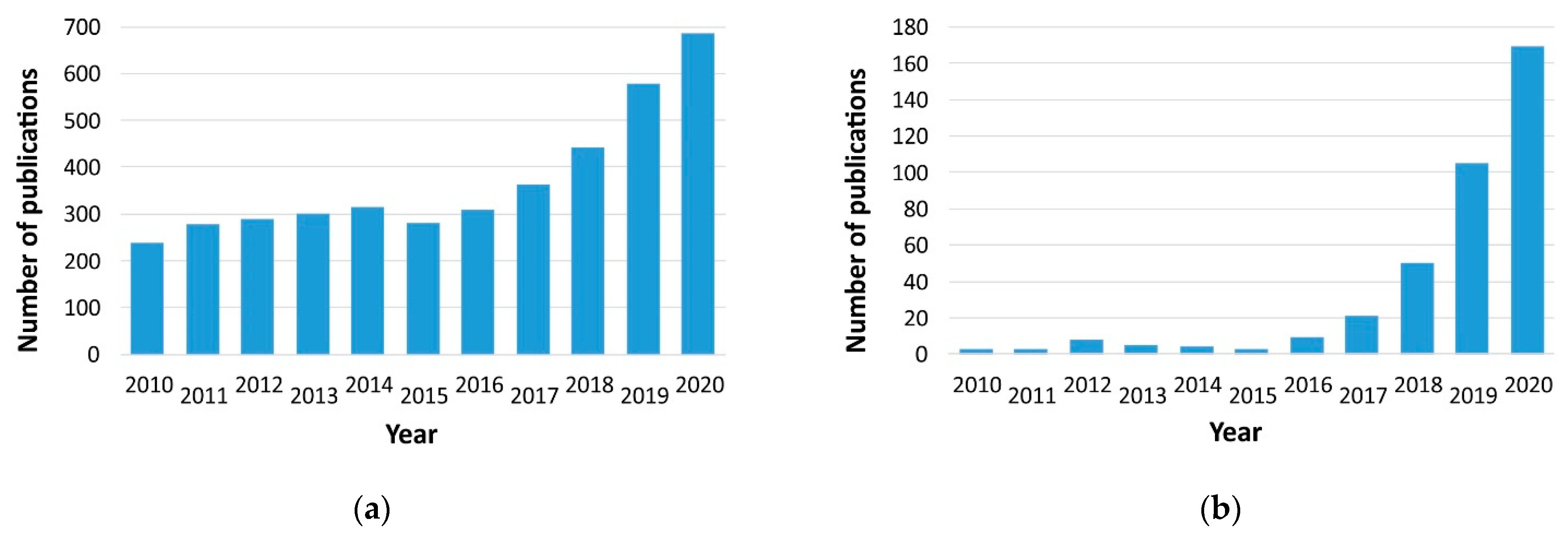
:1. Introduction
2. Neural Networks Design
2.1. Data Set and Neural Network Topology
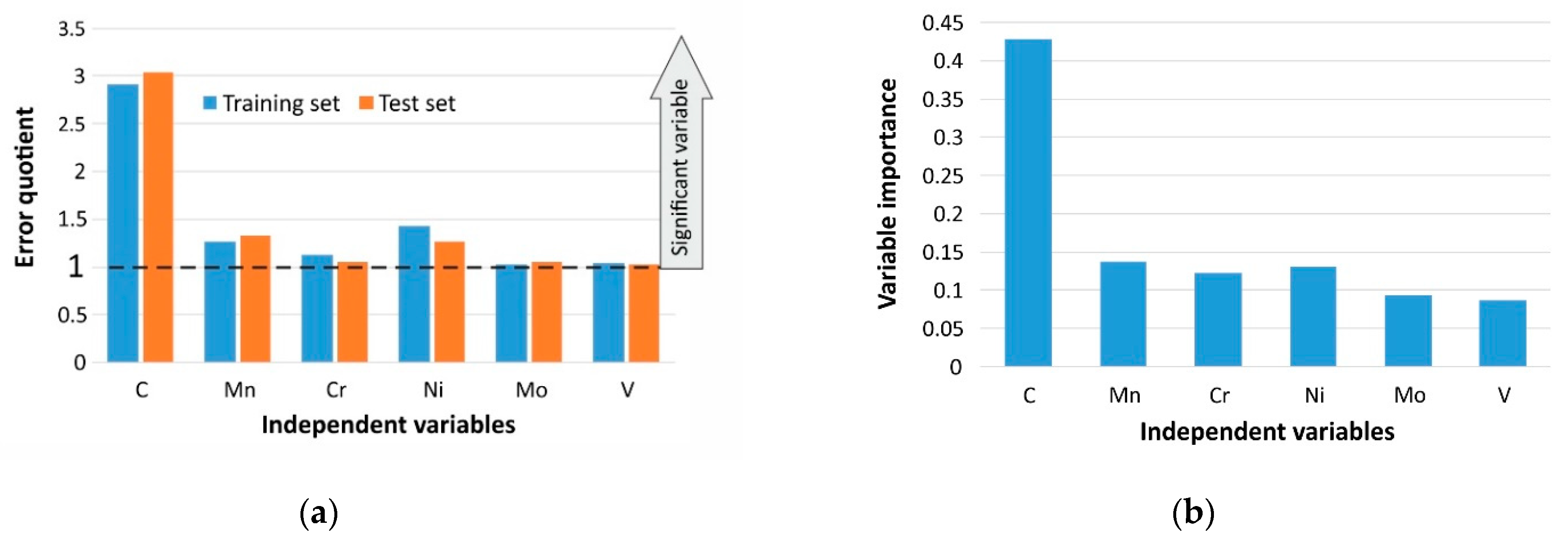
2.2. Independent Variables and Assessment of Their Significance
2.3. Dependent Variables in the Neural Model
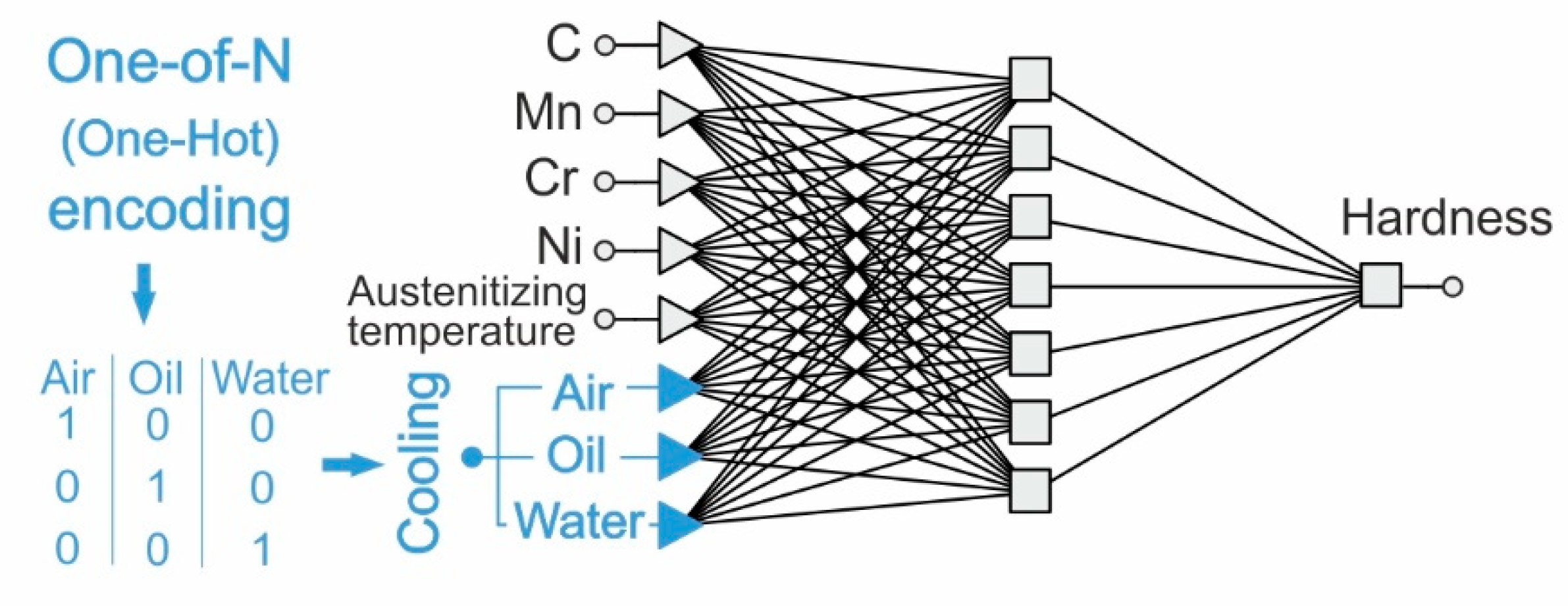
2.4. Qualitative Variables in the Neural Model
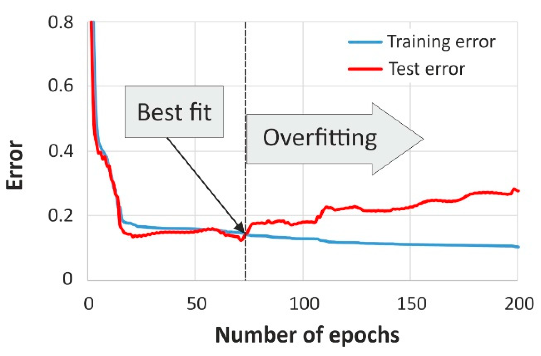
2.5. Model Selection and Overfitting Problem
3. Simulation Using Artificial Neural Network
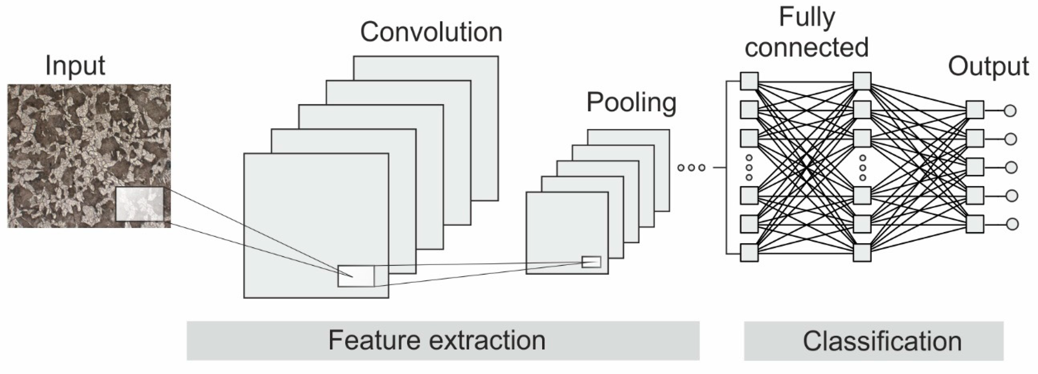
4. Deep Neural Networks
5. Artificial Neural Networks in Hybrid Systems
6. Summary
Author Contributions
Funding
Institutional Review Board Statement
Informed Consent Statement
Conflicts of Interest
References
- Rajan, K. Materials informatics. Mater. Today 2005, 8, 38–45. [Google Scholar] [CrossRef]
- Sha, W.; Guo, Y.; Yuan, Q.; Tang, S.; Zhang, X.; Lu, S.; Guo, X.; Cao, Y.C.; Cheng, S. Artificial Intelligence to Power the Future of Materials Science and Engineering. Adv. Intell. Syst. 2020, 2, 1900143. [Google Scholar] [CrossRef] [Green Version]
- Bhadeshia, H.K.D.H. Mathematical Models in Materials Science. Mater. Sci. Technol. 2008, 24, 128–136. [Google Scholar] [CrossRef]
- Liu, Y.; Zhao, T.; Ju, W.; Shi, S. Materials discovery and design using machine learning. J. Mater. 2017, 3, 159–177. [Google Scholar] [CrossRef]
- Mueller, T.; Kusne, A.G.; Ramprasad, R. Machine Learning in Materials Science: Recent Progress and Emerging Applications. Rev. Comp. Chem. 2016, 29, 186–273. [Google Scholar] [CrossRef]
- Wei, J.; Chu, X.; Sun, X.Y.; Xu, K.; Deng, H.X.; Chen, J.; Wei, Z.; Lei, M. Machine learning in materials science. InfoMat 2019, 1, 338–358. [Google Scholar] [CrossRef]
- Chakraborti, N. Genetic algorithms in materials design and processing. Int. Mater. Rev. 2004, 49, 246–260. [Google Scholar] [CrossRef]
- Datta, S. Materials Design Using Computational Intelligence Techniques; CRC Press: Boca Raton, FL, USA, 2016. [Google Scholar]
- Datta, S.; Chattopadhyay, P.P. Soft computing techniques in advancement of structural metals. Int. Mater. Rev. 2013, 58, 475–504. [Google Scholar] [CrossRef]
- Sitek, W.; Dobrzański, L.A. Application of genetic methods in materials’ design. J. Mater. Process. Technol. 2005, 164–165, 1607–1611. [Google Scholar] [CrossRef]
- Anderson, J.A. An Introduction to Neural Networks; MIT Press: Cambridge, MA, USA, 1995. [Google Scholar]
- Hassoun, M.H. Fundamentals of Artificial Neural Networks; MIT Press: Cambridge, MA, USA, 1995. [Google Scholar]
- Bishop, C.M. Neural Networks for Pattern Recognition, 1st ed.; Oxford University Press: Oxford, UK, 1995. [Google Scholar]
- Bhadeshia, H.K.D.H. Neural Networks and Information in Materials Science. Stat. Anal. Data Min. 2009, 1, 296–304. [Google Scholar] [CrossRef]
- Bhadeshia, H.K.D.H. Neural Networks in Materials Science. ISIJ Int. 1999, 39, 966–979. [Google Scholar] [CrossRef]
- Sha, W.; Edwards, K.L. The use of artificial neural networks in materials science based research. Mater. Des. 2007, 28, 1747–1752. [Google Scholar] [CrossRef]
- Bhadeshia, H.K.D.H.; Dimitriu, R.C.; Forsik, S.; Pak, J.H.; Ryu, J.H. Performance of neural networks in materials science. Mater. Sci. Technol. 2009, 25, 504–510. [Google Scholar] [CrossRef] [Green Version]
- Mukherjee, M.; Singh, S.B. Artificial Neural Network: Some Applications in Physical Metallurgy of Steels. Mater. Manuf. Process. 2009, 24, 198–208. [Google Scholar] [CrossRef]
- Dobrzański, L.A.; Trzaska, J.; Dobrzańska-Danikiewicz, A.D. Use of Neural Networks and Artificial Intelligence Tools for Modeling, Characterization, and Forecasting in Material Engineering, Comprehensive Materials Processing. In Materials Modelling and Characterization; Hashmi, S., Ed.; Elsevier Science: Amsterdam, The Netherlands, 2014; Volume 2, pp. 161–198. [Google Scholar]
- Agrawal, A.; Choudhary, A. Deep materials informatics: Applications of deep learning in materials science. MRS Commun. 2019, 9, 779–792. [Google Scholar] [CrossRef] [Green Version]
- Bock, F.E.; Aydin, R.C.; Cyron, C.J.; Huber, N.; Kalidindi, S.R.; Klusemann, B. A Review of the Application of Machine Learning and Data Mining Approaches in Continuum Materials Mechanics. Front. Mater. 2009, 6, 110. [Google Scholar] [CrossRef] [Green Version]
- Hong, Y.; Hou, B.; Jiang, H.; Zhang, J. Machine learning and artificial neural network accelerated computational discoveries in materials science. WIREs Comput. Mol. Sci. 2020, 10, e1450. [Google Scholar] [CrossRef]
- Schmidt, J.; Marques, M.R.G.; Botti, S.; Marques, M.A.L. Recent advances and applications of machine learning in solid-state materials science. Npj Comput. Mater. 2019, 5, 83. [Google Scholar] [CrossRef]
- Kalidindi, S.R.; Graef, M.D. Materials data science: Current status and future outlook. Ann. Rev. Mater. Res. 2015, 45, 171–193. [Google Scholar] [CrossRef]
- May, R.; Dandy, G.; Maier, H. Review of Input Variable Selection Methods for Artificial Neural Networks. In Artificial Neural Networks—Methodological Advances and Biomedical Applications; Suzuki, K., Ed.; InTech: Rijeka, Croatia, 2011; pp. 19–44. [Google Scholar]
- Trzaska, J. Prediction Methodology for the Anisothermal Phase Transformation Curves of the Structural and Engineering Steels; Silesian University of Technology Press: Gliwice, Poland, 2017. (In Polish) [Google Scholar]
- Trzaska, J. A new neural networks model for calculating the continuous cooling transformation diagrams. Arch. Metall. Mater. 2018, 63, 2009–2015. [Google Scholar] [CrossRef]
- Rahaman, M.; Mu, W.; Odqvist, J.; Hedstrom, P. Machine Learning to Predict the Martensite Start Temperature in Steels. Metall. Mater. Trans. A 2019, 50, 2081–2091. [Google Scholar] [CrossRef] [Green Version]
- Krajewski, S.; Nowacki, J. Dual-phase steels microstructure and properties consideration based on artificial intelligence techniques. Arch. Civ. Mech. Eng. 2014, 14, 278–286. [Google Scholar] [CrossRef]
- Merayo, D.; Rodríguez-Prieto, A.; Camacho, A.M. Prediction of Mechanical Properties by Artificial Neural Networks to Characterize the Plastic Behavior of Aluminum Alloys. Materials 2020, 13, 5227. [Google Scholar] [CrossRef] [PubMed]
- Kemp, R.; Cottrell, G.A.; Bhadeshia, H.K.D.H.; Odette, G.R.; Yamamoto, T.; Kishimoto, H. Neural-network analysis of irradiation hardening in low-activation steels. J. Nucl. Mater. 2006, 348, 311–328. [Google Scholar] [CrossRef] [Green Version]
- Yescas, M.A. Prediction of the Vickers hardness in austempered ductile irons using neural networks. Int. J. Cast Metals Res. 2003, 15, 513–521. [Google Scholar] [CrossRef]
- Sourmail, T.; Bhadeshia, H.K.D.H.; MacKay, D.J.C. Neural network model of creep strength of austenitic stainless steels. Mater. Sci. Technol. 2002, 18, 655–663. [Google Scholar] [CrossRef]
- Sitek, W. Methodology of High-Speed Steels Design Using the Artificial Intelligence Tools. J. Achiev. Mater. Manuf. Eng. 2010, 39, 115–160. [Google Scholar]
- Singh, K.; Rajput, S.K.; Mehta, Y. Modeling of the hot deformation behavior of a high phosphorus steel using artificial neural networks. Mater. Discov. 2016, 6, 1–8. [Google Scholar] [CrossRef]
- Kumar, S.; Karmakar, A.; Nath, S.K. Construction of hot deformation processing maps for 9Cr-1Mo steel through conventional and ANN approach. Mater. Today Commun. 2021, 26, 101903. [Google Scholar] [CrossRef]
- Murugesan, M.; Sajjad, M.; Jung, D.W. Hybrid Machine Learning Optimization Approach to Predict Hot Deformation Behavior of Medium Carbon Steel Material. Metals 2019, 9, 1315. [Google Scholar] [CrossRef] [Green Version]
- Reddy, N.S.; Krishnaiah, J.; Young, H.B.; Lee, J.S. Design of medium carbon steels by computational intelligence techniques. Comp. Mater. Sci. 2015, 101, 120–126. [Google Scholar] [CrossRef]
- Reddy, N.S.; Panigrahi, B.B.; Ho, C.M.; Kim, J.H.; Lee, C.S. Artificial neural network modeling on the relative importance of alloying elements and heat treatment temperature to the stability of α and β phase in titanium alloys. Comp. Mater. Sci. 2015, 107, 175–183. [Google Scholar] [CrossRef]
- Narayana, P.L.; Lee, S.W.; Park, C.H.; Yeom, J.T.; Hong, J.K.; Maurya, A.K.; Reddy, N.S. Modeling high-temperature mechanical properties of austenitic stainless steels by neural networks. Comp. Mater. Sci. 2020, 179, 109617. [Google Scholar] [CrossRef]
- Dehghani, K.; Nekahi, A. Artificial neural network to predict the effect of thermomechanical treatments on bake hardenability of low carbon steels. Mater. Des. 2010, 31, 2224–2229. [Google Scholar] [CrossRef]
- Liu, Y.; Zhu, J.; Cao, Y. Modeling effects of alloying elements and heat treatment parameters on mechanical properties of hot die steel with back-propagation artificial neural network. J. Iron Steel Res. Int. 2017, 24, 1254–1260. [Google Scholar] [CrossRef]
- Khalaj, G.; Nazariy, A.; Pouraliakbar, H. Prediction of martensite fraction of microalloyed steel by artificial neural networks. Neural Netw. World 2013, 2, 117–130. [Google Scholar] [CrossRef] [Green Version]
- Sandhya, N.; Sowmya, V.; Bandaru, C.R.; Raghu Babu, G. Prediction of Mechanical Properties of Steel using Data Science Techniques. Int. J. Recent Technol. Eng. 2019, 8, 235–241. [Google Scholar] [CrossRef]
- Olden, J.D.; Joy, M.K.; Death, R.G. An accurate comparison of methods for quantifying variable importance in artificial neural networks sing simulated data. Ecol. Model. 2004, 178, 389–397. [Google Scholar] [CrossRef]
- Wang, Y.; Wu, X.; Li, X.; Xie, Z.; Liu, R.; Liu, W.; Zhang, Y.; Xu, Y.; Liu, C. Prediction and Analysis of Tensile Properties of Austenitic Stainless Steel Using Artificial Neural Network. Metals 2020, 10, 234. [Google Scholar] [CrossRef] [Green Version]
- Cai, Z.; Ji, H.; Pei, W.; Tang, X.; Xin, L.; Lu, Y.; Li, W. An Investigation into the Dynamic Recrystallization (DRX) Behavior and Processing Map of 33Cr23Ni8Mn3N Based on an Artificial Neural Network (ANN). Materials 2020, 13, 1282. [Google Scholar] [CrossRef] [Green Version]
- Kocaman, E.; Sirin, S.; Dispinar, D. Artificial Neural Network Modeling of Grain Refinement Performance in AlSi10Mg Alloy. Inter. J. Metalcast. 2021, 15, 338–348. [Google Scholar] [CrossRef]
- Holland, J.H. Adaptation in Natural and Artificial Systems: An Introductory Analysis with Applications to Biology, Control, and Artificial Intelligence; U Michigan Press: Ann Arbor, MI, USA, 1975. [Google Scholar]
- Goldberg, D.E. Genetic Algorithms in Search, Optimization and Machine Learning, 1st ed.; Addison-Wesley Longman Publishing Co.: Boston, MA, USA, 1989. [Google Scholar]
- Honysz, R. Optimization of ferrite stainless steel mechanical properties prediction with artificial intelligence algorithms. Arch. Metall. Mater. 2020, 65, 749–753. [Google Scholar] [CrossRef]
- Powar, A.; Date, P. Modeling of microstructure and mechanical properties of heat treated components by using Artificial Neural Network. Mat. Sci. Eng. A-Struct. 2015, 628, 89–97. [Google Scholar] [CrossRef]
- Chakraborty, S.; Chattopadhyay, P.P.; Ghosh, S.K.; Datta, S. Incorporation of prior knowledge in neural network model for continuous cooling of steel using genetic algorithm. Appl. Soft. Comput. 2017, 58, 297–306. [Google Scholar] [CrossRef]
- Smoljan, B.; Smokvina Hanza, S.; Tomašić, N.; Iljkić, D. Computer simulation of microstructure transformation in heat treatment processes. J. Achiev. Mater. Manuf. Eng. 2007, 24, 275–282. [Google Scholar]
- Xia, X.; Nie, J.F.; Davies, C.H.J.; Tang, W.N.; Xu, S.W.; Birbilis, N. An artificial neural network for predicting corrosion rate and hardness of magnesium alloys. Mater. Design 2016, 90, 1034–1043. [Google Scholar] [CrossRef]
- Dutta, T.; Dey, S.; Datta, S.; Das, D. Designing dual-phase steels with improved performance using ANN and GA in tandem. Comp. Mater. Sci. 2019, 157, 6–16. [Google Scholar] [CrossRef]
- Yetim, A.F.; Codur, M.Y.; Yazici, M. Using of artificial neural network for the prediction of tribological properties of plasma nitride 316L stainless steel. Mater. Lett. 2015, 158, 170–173. [Google Scholar] [CrossRef]
- Dobrzański, J.; Sroka, M.; Zieliński, A. Methodology of classification of internal damage the steels during creep service. J. Achiev. Mater. Manuf. Eng. 2006, 18, 263–266. [Google Scholar]
- Trzaska, J.; Sitek, W.; Dobrzański, L.A. Application of neural networks for selection of steel grade with required hardenability. Int. J. Comput. Mater. Sci. Surf. Eng. 2007, 1, 336–382. [Google Scholar] [CrossRef]
- Trzaska, J. Examples of simulation of the alloying elements effect on austenite transformations during continuous cooling. Arch. Metall. Mater. 2021, 66, 331–337. [Google Scholar] [CrossRef]
- Sidhu, G.; Bhole, S.D.; Chen, D.L.; Essadiqi, E. Determination of volume fraction of bainite in low carbon steels using artificial neural networks. Comp. Mater. Sci. 2011, 50, 337–3384. [Google Scholar] [CrossRef]
- Garcia-Mateo, C.; Capdevila, C.; Garcia Caballero, F.; Garcia de Andres, C. Artificial neural network modeling for the prediction of critical transformation temperatures in steels. J. Mater. Sci. 2007, 42, 5391–5397. [Google Scholar] [CrossRef] [Green Version]
- Razavi, A.R.; Ashrafizadeh, F.; Fooladi, S. Prediction of age hardening parameters for 17-4PH stainless steel by artificial neural network and genetic algorithm. Mat. Sci. Eng. A-Struct. 2016, 675, 147–152. [Google Scholar] [CrossRef]
- Reddy, N.S.; Krishnaiah, J.; Hong, S.G.; Lee, J.S. Modeling medium carbon steels by using artificial neural networks. Mat. Sci. Eng. A-Struct. 2009, 508, 93–105. [Google Scholar] [CrossRef]
- Sun, Y.; Zeng, W.; Han, Y.; Ma, X.; Zhao, Y.; Guo, P.; Wang, G.; Dargusch, M.S. Determination of the influence of processing parameters on the mechanical properties of the Ti–6Al–4V alloy using an artificial neural network. Comp. Mater. Sci. 2012, 60, 239–244. [Google Scholar] [CrossRef]
- Bhattacharyya, T.; Singh, S.B.; Sikdar, S.; Bhattacharyya, S.; Bleck, W.; Bhattacharjee, D. Microstructural prediction through artificial neural network (ANN) for development of transformation induced plasticity (TRIP) aided steel. Mat. Sci. Eng. A-Struct. 2013, 565, 148–157. [Google Scholar] [CrossRef]
- Lin, Y.C.; Zhang, J.; Zhong, J. Application of neural networks to predict the elevated temperature flow behavior of a low alloy steel. Comp. Mater. Sci. 2008, 43, 752–758. [Google Scholar] [CrossRef]
- Lin, Y.C.; Liu, G.; Chen, M.S.; Zhong, J. Prediction of static recrystallization in a multi-pass hot deformed low-alloy steel using artificial neural network. J. Mater. Process. Technol. 2009, 209, 4611–4616. [Google Scholar] [CrossRef]
- Monajati, H.; Asefi, D.; Parsapour, A.; Abbasi, S. Analysis of the effects of processing parameters on mechanical properties and formability of cold rolled low carbon steel sheets using neural networks. Comp. Mater. Sci. 2010, 49, 876–881. [Google Scholar] [CrossRef]
- Geng, X.; Wang, H.; Xue, W.; Xiang, S.; Huang, H.; Meng, L.; Ma, G. Modeling of CCT diagrams for tool steels using different machine learning techniques. Comp. Mater. Sci. 2020, 171, 109235. [Google Scholar] [CrossRef]
- Sourmail, T.; Garcia-Mateo, C. Critical assessment of models for predicting the Ms temperature of steels. Comp. Mater. Sci. 2005, 34, 323–334. [Google Scholar] [CrossRef] [Green Version]
- Sitek, W.; Trzaska, J. Numerical Simulation of the Alloying Elements Effect on Steels’ Properties. J. Achiev. Mater. Manuf. Eng. 2011, 45, 71–78. [Google Scholar]
- Sidhu, G.; Bhole, S.D.; Chen, D.L.; Essadiqi, E. Development and experimental validation of a neural network model for prediction and analysis of the strength of bainitic steels. Mater. Des. 2012, 41, 99–107. [Google Scholar] [CrossRef]
- Goodfellow, I.; Bengio, Y.; Courville, A. Deep Learning; MIT Press: Cambridge, MA, USA, 2016. [Google Scholar]
- Azimi, S.M.; Britz, D.; Engstler, M.; Fritz, M.; Mücklich, F. Advanced Steel Microstructural Classification by Deep Learning Methods. Sci. Rep. 2018, 8, 2128. [Google Scholar] [CrossRef]
- Patterson, J.; Gibson, A. Deep Learning. A Practitioner’s Approach, 1st ed.; O’Reilly Media, Inc.: Sebastopol, MA, USA, 2017. [Google Scholar]
- Lenz, B.; Hasselbruch, H.; Mehner, A. Automated evaluation of Rockwell adhesion tests for PVD coatings using convolutional neural networks. Surf. Coat. Technol. 2020, 385, 125365. [Google Scholar] [CrossRef]
- Mulewicz, B.; Korpala, G.; Kusiak, J.; Prahl, U. Autonomous Interpretation of the Microstructure of Steels and Special Alloys. Mater. Sci. Forum 2019, 949, 24–31. [Google Scholar] [CrossRef] [Green Version]
- Wei, R.; Song, Y.; Zhang, Y. Enhanced Faster Region Convolutional Neural Networks for Steel Surface Defect Detection. ISIJ Int. 2020, 60, 539–545. [Google Scholar] [CrossRef] [Green Version]
- Lee, S.Y.; Tama, B.A.; Moon, S.J.; Lee, S. Steel Surface Defect Diagnostics Using Deep Convolutional Neural Network and Class Activation Map. Appl. Sci. 2019, 9, 5449. [Google Scholar] [CrossRef] [Green Version]
- Krizhevsky, A.; Sutskever, I.; Hinton, G. ImageNet classification with deep convolutional neural networks. Commun. ACM 2017, 60, 84–90. [Google Scholar] [CrossRef]
- Gao, Y.; Gao, L.; Li, X.; Yan, X. A semi-supervised convolutional neural network-based method for steel surface defect recognition. Robot. Comput.-Integr. Manuf. 2020, 61, 101825. [Google Scholar] [CrossRef]
- Yi, L.; Li, G.; Jiang, M. An End-to-End Steel Strip Surface Defects Recognition System Based on Convolutional Neural Networks. Steel Res. Int. 2017, 88, 1600068. [Google Scholar] [CrossRef]
- Konovalenko, I.; Maruschak, P.; Brezinová, J.; Viňáš, J.; Brezina, J. Steel Surface Defect Classification Using Deep Residual Neural Network. Metals 2020, 10, 846. [Google Scholar] [CrossRef]
- Wang, S.; Xia, X.; Ye, L.; Yang, B. Automatic Detection and Classification of Steel Surface Defect Using Deep Convolutional Neural Networks. Metals 2021, 11, 388. [Google Scholar] [CrossRef]
- He, D.; Xu, K.; Wang, D. Design of multi-scale receptive field convolutional neural network for surface inspection of hot rolled steels. Image Vision Comput. 2019, 89, 12–20. [Google Scholar] [CrossRef]
- Zhang, S.; Zhang, Q.; Gu, J.; Su, L.; Li, K.; Pecht, M. Visual inspection of steel surface defects based on domain adaptation and adaptive convolutional neural network. Mech. Syst. Signal Pract. 2021, 153, 107541. [Google Scholar] [CrossRef]
- Choudhury, A.; Pal, S.; Naskar, R.; Basumallick, A. Computer vision approach for phase identification from steel microstructure. Eng. Comput. 2019, 36, 1913–1933. [Google Scholar] [CrossRef]
- Sitek, W.; Trzaska, J. Hybrid Modelling Methods in Materials Science—Selected Examples. J. Achiev. Mater. Manuf. Eng. 2012, 54, 93–102. [Google Scholar]
- Sinha, A.; Sikdar, S.; Chattopadhyay, P.P.; Datta, S. Optimization of mechanical property and shape recovery behavior of Ti-(~49 at.%) Ni alloy using artificial neural network and genetic algorithm. Mater. Design. 2013, 46, 227–234. [Google Scholar] [CrossRef]
- Zhu, Z.; Liang, Y.; Zou, J. Modeling and Composition Design of Low-Alloy Steel’s Mechanical Properties Based on Neural Networks and Genetic Algorithms. Materials 2020, 13, 5316. [Google Scholar] [CrossRef]
- Song, R.G.; Zhang, Q.Z. Heat treatment optimization for 7175 aluminum alloy by genetic algorithm. Mater. Sci. Eng. C 2001, 17, 133–137. [Google Scholar] [CrossRef]
- Mousavi Anijdan, S.H.; Bahrami, A.; Madaah Hosseini, H.R.; Shafyei, A. Using genetic algorithm and artificial neural network analyses to design an Al–Si casting alloy of minimum porosity. Mater. Des. 2006, 27, 605–609. [Google Scholar] [CrossRef]
- Pattanayak, S.; Dey, S.; Chatterjee, S.; Chowdhury, S.G.; Datta, S. Computational intelligence based designing of microalloyed pipeline steel. Comp. Mater. Sci. 2015, 104, 60–68. [Google Scholar] [CrossRef]
- Shahani, A.R.; Setayeshi, S.; Nodamaie, S.A.; Asadi, M.A.; Rezaie, S. Prediction of influence parameters on the hot rolling process using finite element method and neural network. J. Mater. Process. Technol. 2009, 209, 1920–1935. [Google Scholar] [CrossRef]
- Guo, Z.Y.; Sun, J.N.; Du, F.S. Application of finite element method and artificial neural networks to predict the rolling force in hot rolling of Mg alloy plates. J. S. Afr. Inst. Min. Metall. 2016, 116, 43–48. [Google Scholar] [CrossRef] [Green Version]
- Sitek, W.; Trzaska, J.; Dobrzański, L.A. Modified Tartagli method for calculation of Jominy hardenability curve. Mater. Sci. Forum 2008, 575–578, 892–897. [Google Scholar] [CrossRef]
- Tartaglia, J.M.; Eldis, G.T.; Geissler, J.J. Hyperbolic secant method for predicting Jominy hardenability. Metall. Trans. 1984, 15, 1173–1183. [Google Scholar] [CrossRef]
- Trzaska, J.; Dobrzański, L.A. Modelling of CCT diagrams for engineering and constructional steels. J. Mater. Process. Technol. 2007, 192–193, 504–510. [Google Scholar] [CrossRef]

Publisher’s Note: MDPI stays neutral with regard to jurisdictional claims in published maps and institutional affiliations. |
© 2021 by the authors. Licensee MDPI, Basel, Switzerland. This article is an open access article distributed under the terms and conditions of the Creative Commons Attribution (CC BY) license (https://creativecommons.org/licenses/by/4.0/).
Share and Cite
Sitek, W.; Trzaska, J. Practical Aspects of the Design and Use of the Artificial Neural Networks in Materials Engineering. Metals 2021, 11, 1832. https://doi.org/10.3390/met11111832
Sitek W, Trzaska J. Practical Aspects of the Design and Use of the Artificial Neural Networks in Materials Engineering. Metals. 2021; 11(11):1832. https://doi.org/10.3390/met11111832
Chicago/Turabian StyleSitek, Wojciech, and Jacek Trzaska. 2021. "Practical Aspects of the Design and Use of the Artificial Neural Networks in Materials Engineering" Metals 11, no. 11: 1832. https://doi.org/10.3390/met11111832
APA StyleSitek, W., & Trzaska, J. (2021). Practical Aspects of the Design and Use of the Artificial Neural Networks in Materials Engineering. Metals, 11(11), 1832. https://doi.org/10.3390/met11111832