
How Austenitic Is a Martensitic Steel Produced by Laser Powder Bed Fusion? A Cautionary Tale


 and
and
Abstract
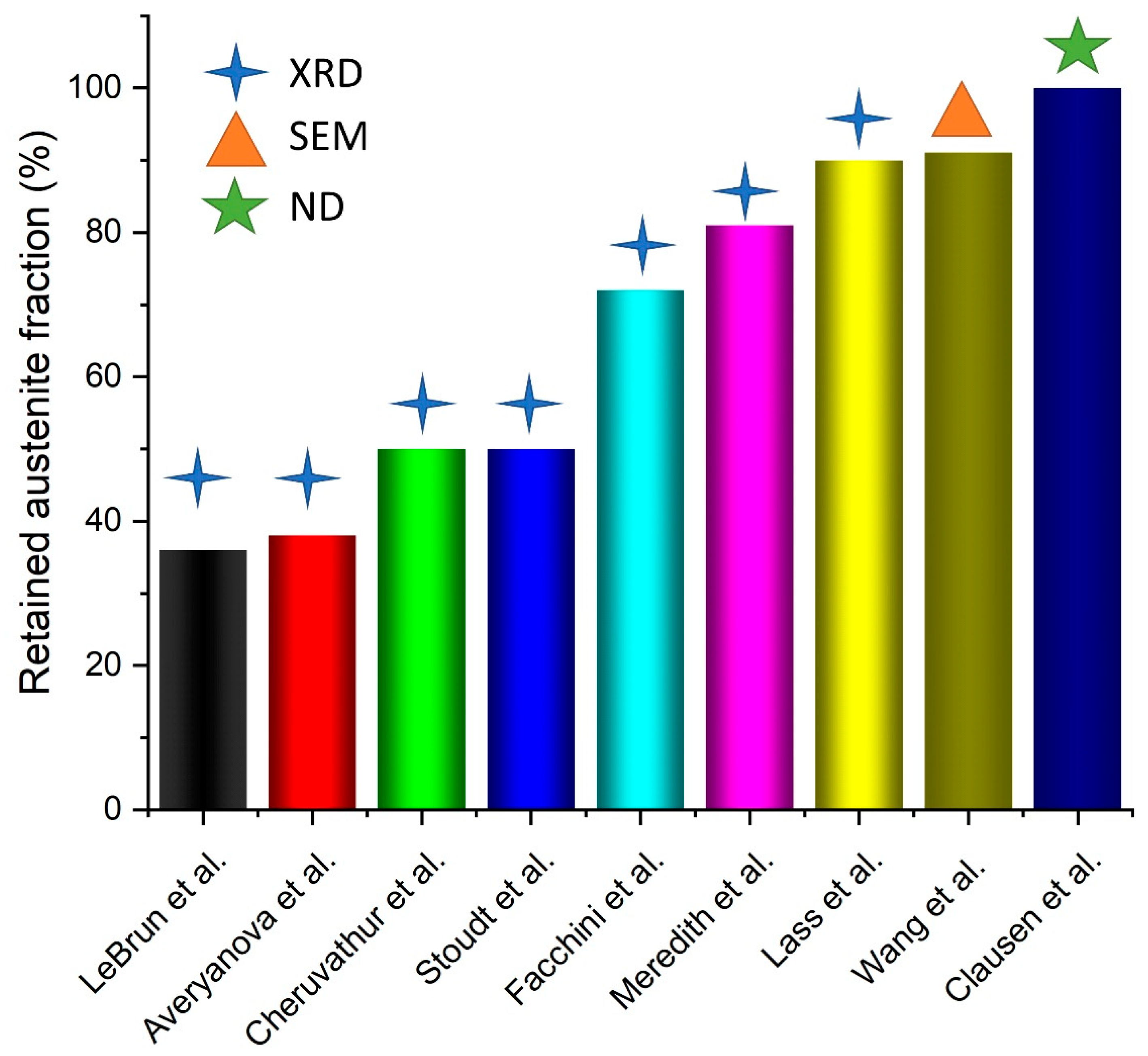
:1. Introduction
2. Materials and Methods
2.1. Materials
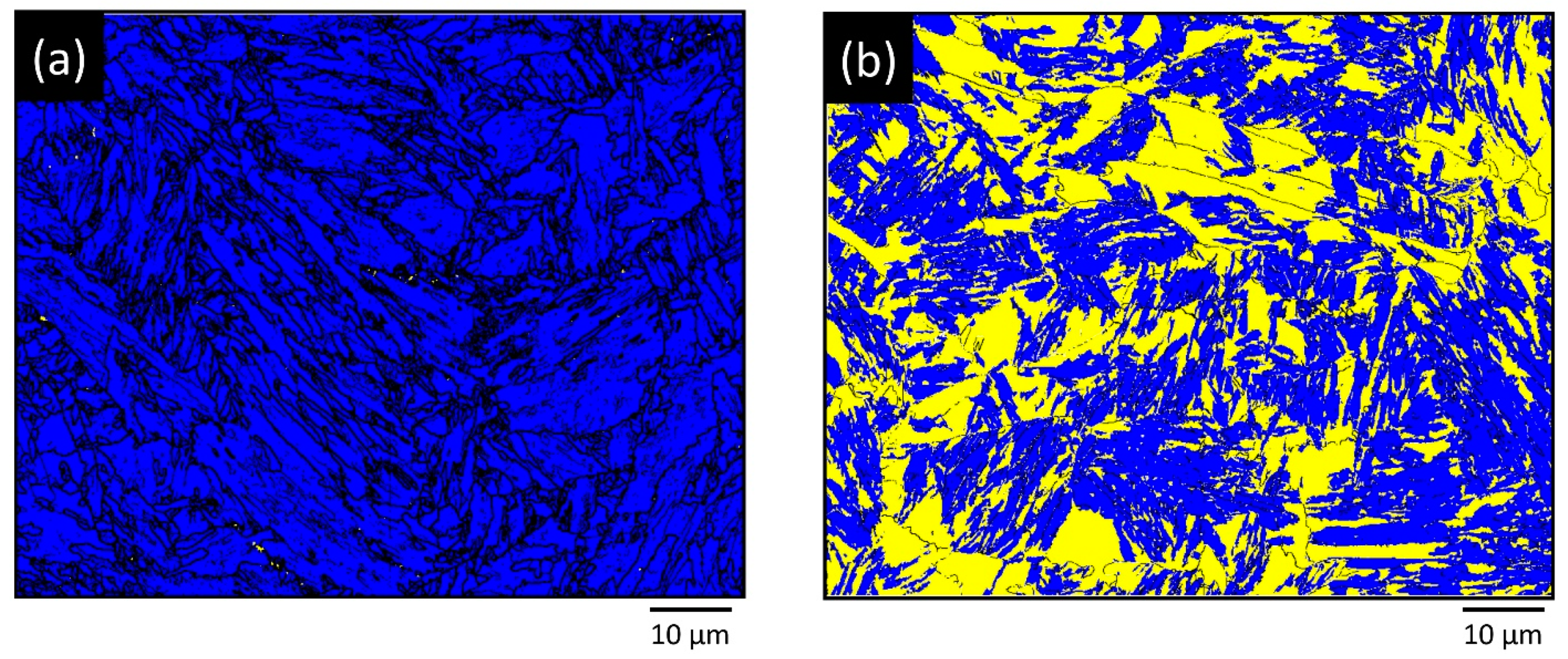
2.2. Electron Backscatter Diffraction Measurements
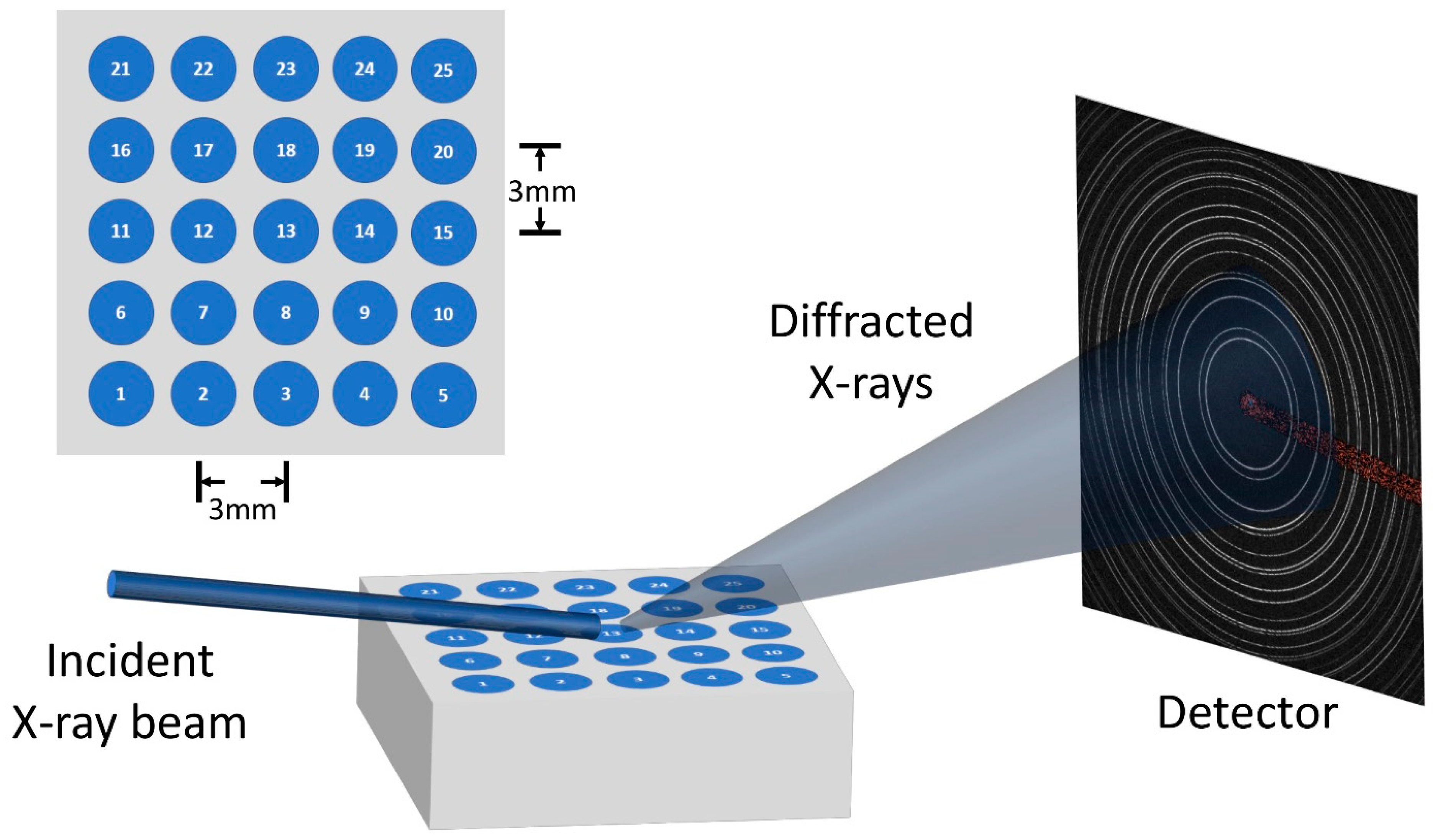
2.3. In-House X-ray Diffraction Measurement with a Cu Source
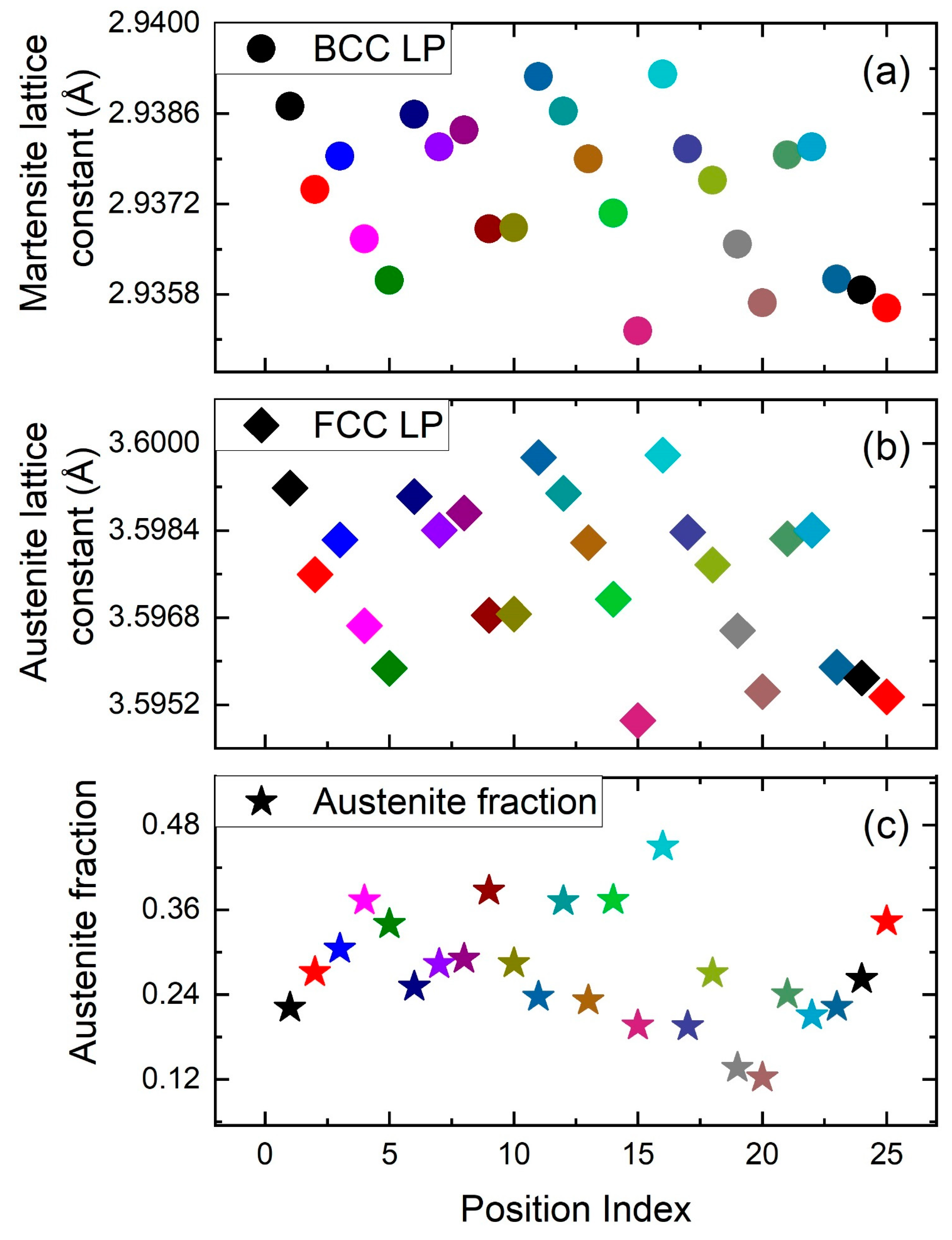
2.4. High-Energy X-ray Diffraction Measurements with a Synchrotron Source
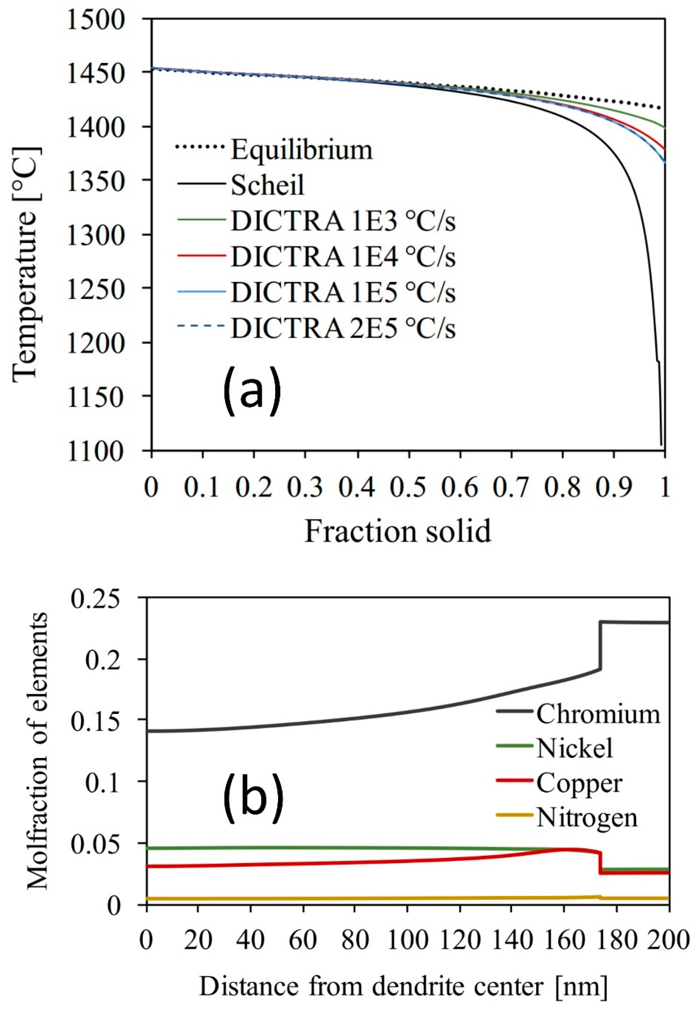
2.5. Calphad Modeling
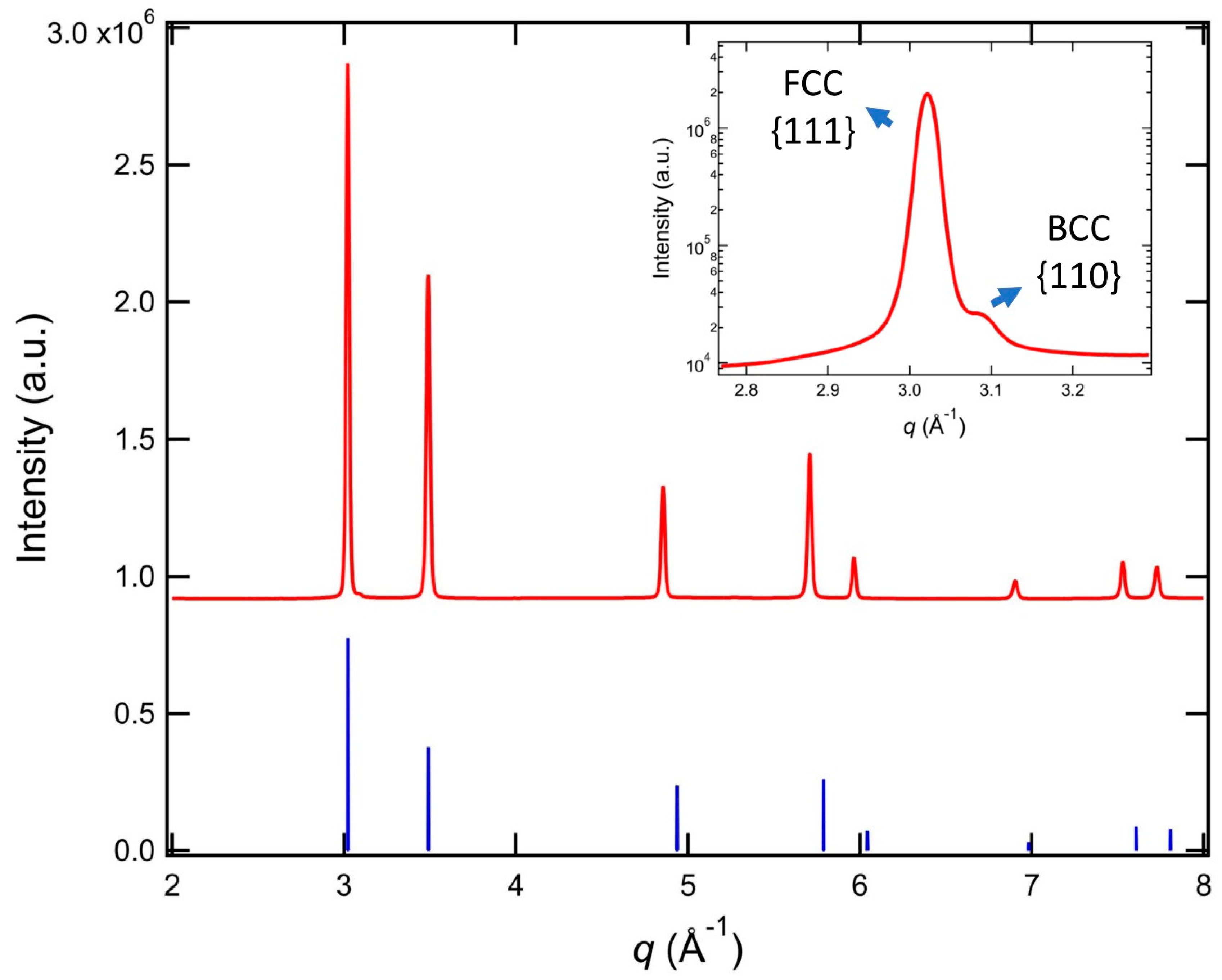
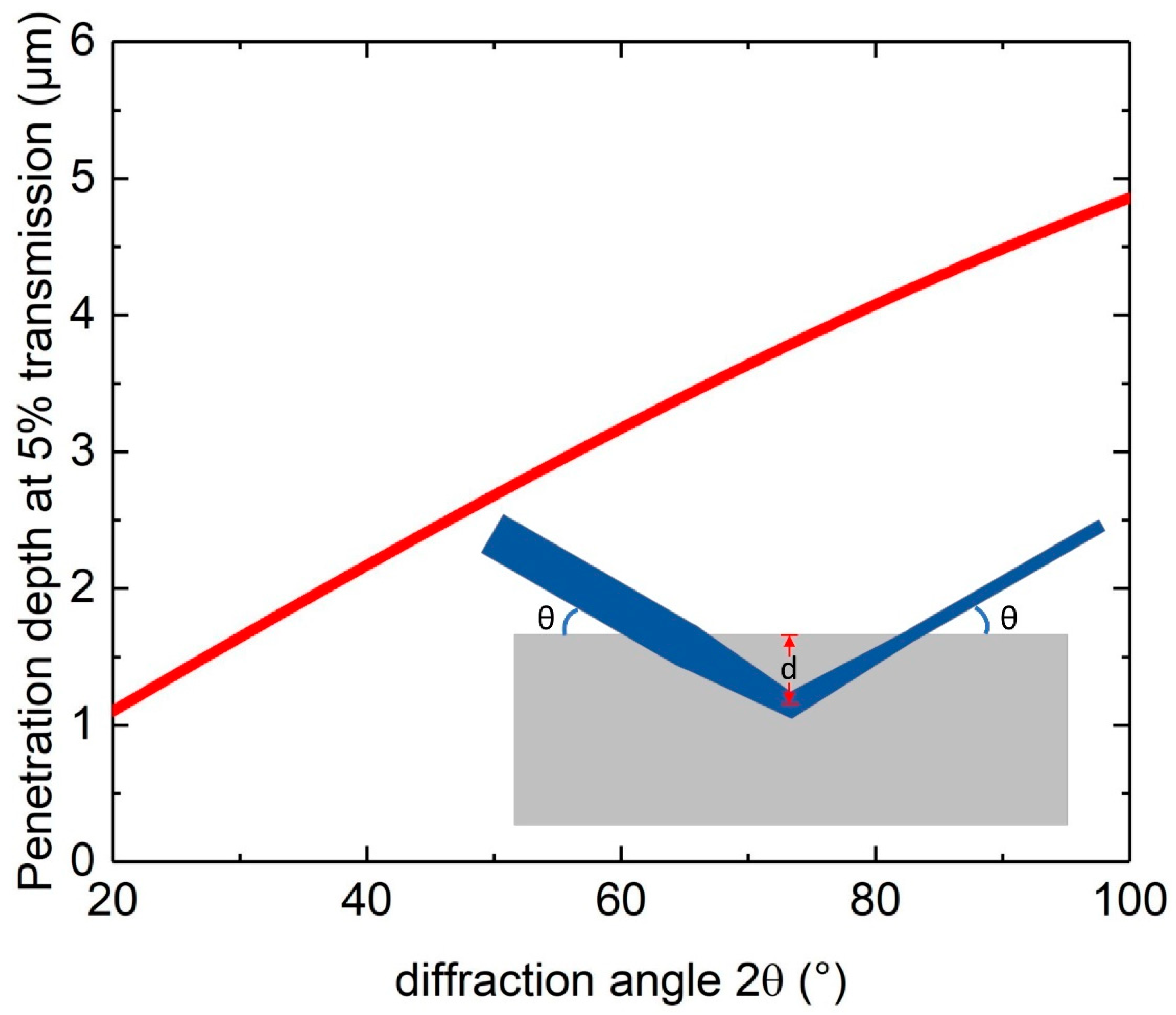
3. Results and Discussions
4. Conclusions
Author Contributions
Funding
Data Availability Statement
Acknowledgments
Conflicts of Interest
References
- Campbell, C.E.; Stoudt, M.R.; Zhang, F. Additive manufacturing of steels and stainless steels. In Additive Manufacturing Processes; Bourell, D.L., Frazier, W., Kuhn, H., Seifi, M., Eds.; ASM International: Materials Park, OH, USA, 2020. [Google Scholar]
- Tofail, S.A.; Koumoulos, E.P.; Bandyopadhyay, A.; Bose, S.; O’Donoghue, L.; Charitidis, C. Additive manufacturing: Scientific and technological challenges, market uptake and opportunities. Mater. Today 2018, 21, 22–37. [Google Scholar] [CrossRef]
- Pereira, T.; Kennedy, J.V.; Potgieter, J. A comparison of traditional manufacturing vs additive manufacturing, the best method for the job. Procedia Manuf. 2019, 30, 11–18. [Google Scholar] [CrossRef]
- Khorasani, M.; Ghasemi, A.; Rolfe, B.; Gibson, I. Additive manufacturing a powerful tool for the aerospace industry. Rapid Prototyp. J. 2021. [Google Scholar] [CrossRef]
- Okamoto, H.; Schlesinger, M.E.; Mueller, E.M. Alloy Phase Diagrams; ASM International: Materials Park, OH, USA, 2016. [Google Scholar]
- Xu, W.; Brandt, M.; Sun, S.; Elambasseril, J.; Liu, Q.; Latham, K.; Xia, K.; Qian, M. Additive manufacturing of strong and ductile Ti–6Al–4V by selective laser melting via in situ martensite decomposition. Acta Mater. 2015, 85, 74–84. [Google Scholar] [CrossRef]
- Facchini, L.; Vicente, N.; Lonardelli, I.; Magalini, E.; Robotti, P.; Molinari, A. Metastable Austenite in 17-4 Precipitation-Hardening Stainless Steel Produced by Selective Laser Melting. Adv. Eng. Mater. 2010, 12, 184–188. [Google Scholar] [CrossRef]
- Alam, M.K.; Mehdi, M.; Urbanic, R.J.; Edrisy, A. Mechanical behavior of additive manufactured AISI 420 martensitic stainless steel. Mater. Sci. Eng. A 2020, 773, 138815. [Google Scholar] [CrossRef]
- Lehnert, R.; Wagner, R.; Burkhardt, C.; Clausnitzer, P.; Weidner, A.; Wendler, M.; Volkova, O.; Biermann, H. Microstructural and mechanical characterization of high-alloy quenching and partitioning TRIP steel manufactured by electron beam melting. Mater. Sci. Eng. A 2020, 794, 139684. [Google Scholar] [CrossRef]
- Zhang, F.; Levine, L.E.; Allen, A.J.; Stoudt, M.R.; Lindwall, G.; Lass, E.A.; Williams, M.E.; Idell, Y.; Campbell, C.E. Effect of heat treatment on the microstructural evolution of a nickel-based superalloy additive-manufactured by laser powder bed fusion. Acta Mater. 2018, 152, 200–214. [Google Scholar] [CrossRef] [PubMed]
- Stoudt, M.R.; Lass, E.; Ng, D.S.; Williams, M.E.; Zhang, F.; Campbell, C.E.; Lindwall, G.; Levine, L.E. The Influence of Annealing Temperature and Time on the Formation of δ-Phase in Additively-Manufactured Inconel 625. Met. Mater. Trans. A 2018, 49, 3028–3037. [Google Scholar] [CrossRef] [Green Version]
- Raghavan, S.; Zhang, B.; Wang, P.; Sun, C.-N.; Nai, M.L.S.; Li, T.; Wei, J. Effect of different heat treatments on the microstructure and mechanical properties in selective laser melted INCONEL 718 alloy. Mater. Manuf. Process. 2016, 32, 1588–1595. [Google Scholar] [CrossRef]
- Zuback, J.; Moradifar, P.; Khayat, Z.; Alem, N.; Palmer, T. Impact of chemical composition on precipitate morphology in an additively manufactured nickel base superalloy. J. Alloys Compd. 2019, 798, 446–457. [Google Scholar] [CrossRef]
- Zhang, F.; Ilavsky, J.; Lindwall, G.; Stoudt, M.R.; Levine, L.E.; Allen, A.J. Solid-State Transformation of an Additive Manufactured Inconel 625 Alloy at 700 °C. Appl. Sci. 2021, 11, 8643. [Google Scholar] [CrossRef]
- Di Schino, A. Manufacturing and Applications of Stainless Steels. Metals 2020, 10, 327. [Google Scholar] [CrossRef] [Green Version]
- Ilavsky, J.; Jemian, P.R. Irena: Tool suite for modeling and analysis of small-angle scattering. J. Appl. Crystallogr. 2009, 42, 347–353. [Google Scholar] [CrossRef]
- Toby, B.; Von Dreele, R.B. GSAS-II: The genesis of a modern open-source all purpose crystallography software package. J. Appl. Crystallogr. 2013, 46, 544–549. [Google Scholar] [CrossRef]
- Borkiewicz, O.J.; Ruett, U.; Beyer, K.; Gallington, L. New capabilities at beamline 11-ID-B of the Advanced Photon Source. Acta Crystallogr. Sect. A Found. Adv. 2019, 75, a352. [Google Scholar] [CrossRef]
- Cline, J.; Filliben, J.; Von Dreele, R.; Winburn, R.; Stephens, P. D-90 Addressing the Amorphous Content Issue in Quantitative Phase Analysis: The Certification of NIST SRM 676A. Powder Diffr. 2009, 24, 172. [Google Scholar] [CrossRef]
- Andersson, J.-O.; Helander, T.; Höglund, L.; Shi, P.; Sundman, B. Thermo-Calc & DICTRA, computational tools for materials science. Calphad 2002, 26, 273–312. [Google Scholar] [CrossRef]
- Gulliver, G. The quantitative effect of rapid cooling upon the constitution of binary alloys. J. Inst. Met. 1913, 9, 120–157. [Google Scholar]
- Steels, T.-T. Fe-Alloys Database Version 7.0; Thermo-Calc Software: Solna, Sweden, 2012. [Google Scholar]
- Liu, S.; Shin, Y.C. Additive manufacturing of Ti6Al4V alloy: A review. Mater. Des. 2019, 164, 107552. [Google Scholar] [CrossRef]
- Popovich, V.; Borisov, E.; Sufiiarov, V.; Masaylo, D.; Alzina, L. Functionally graded Inconel 718 processed by additive manufacturing: Crystallographic texture, anisotropy of microstructure and mechanical properties. Mater. Des. 2017, 114, 441–449. [Google Scholar] [CrossRef]
- Jia, Q.; Zhang, F.; Rometsch, P.; Li, J.; Mata, J.; Weyland, M.; Bourgeois, L.; Sui, M.; Wu, X. Precipitation kinetics, microstructure evolution and mechanical behavior of a developed Al–Mn–Sc alloy fabricated by selective laser melting. Acta Mater. 2020, 193, 239–251. [Google Scholar] [CrossRef]
- Le Brun, T.; Nakamoto, T.; Horikawa, K.; Kobayashi, H. Effect of retained austenite on subsequent thermal processing and re-sultant mechanical properties of selective laser melted 17–4 ph stainless steel. Mater. Design 2015, 81, 44–53. [Google Scholar] [CrossRef]
- Averyanova, M.; Bertrand, P.; Verquin, B. Effect of initial powder properties on final microstructure and mechanical properties of parts manufactured by selective laser melting. In Proceedings of the Annals of DAAAM for 2010 & Proceedings of the 21st International DAAAM Symposium, Zadar, Croatia, 20–23 October 2010. [Google Scholar]
- Cheruvathur, S.; Lass, E.A.; Campbell, C.E. Additive Manufacturing of 17-4 PH Stainless Steel: Post-processing Heat Treatment to Achieve Uniform Reproducible Microstructure. JOM 2016, 68, 930–942. [Google Scholar] [CrossRef]
- Stoudt, M.R.; Ricker, R.E.; Lass, E.; Levine, L.E. Influence of postbuild microstructure on the electrochemical behavior of additively manufactured 17-4 ph stainless steel. JOM 2017, 69, 506–515. [Google Scholar] [CrossRef] [Green Version]
- Meredith, S.; Zuback, J.; Keist, J.; Palmer, T. Impact of composition on the heat treatment response of additively manufactured 17–4 PH grade stainless steel. Mater. Sci. Eng. A 2018, 738, 44–56. [Google Scholar] [CrossRef]
- Lass, E.A.; Zhang, F.; Campbell, C.E. Nitrogen Effects in Additively Manufactured Martensitic Stainless Steels: Conventional Thermal Processing and Comparison with Wrought. Met. Mater. Trans. A 2020, 51, 2318–2332. [Google Scholar] [CrossRef]
- Wang, X.; Liu, Y.; Shi, T.; Wang, Y. Strain rate dependence of mechanical property in a selective laser melted 17–4 PH stainless steel with different states. Mater. Sci. Eng. A 2020, 792, 139776. [Google Scholar] [CrossRef]
- Clausen, B.; Brown, D.; Carpenter, J.; Clarke, K.; Clarke, A.; Vogel, S.; Bernardin, J.; Spernjak, D.; Thompson, J. Deformation behavior of additively manufactured GP1 stainless steel. Mater. Sci. Eng. A 2017, 696, 331–340. [Google Scholar] [CrossRef] [Green Version]
- Zhang, F.; Levine, L.E.; Allen, A.J.; Young, S.W.; Williams, M.E.; Stoudt, M.R.; Moon, K.-W.; Heigel, J.C.; Ilavsky, J. Phase Fraction and Evolution of Additively Manufactured (AM) 15-5 Stainless Steel and Inconel 625 AM-Bench Artifacts. Integr. Mater. Manuf. Innov. 2019, 8, 362–377. [Google Scholar] [CrossRef]
- Lindwall, G.; Campbell, C.; Lass, E.; Zhang, F.; Stoudt, M.R.; Allen, A.J.; Levine, L.E. Simulation of ttt curves for additively man-ufactured inconel 625. Metall. Mater. Trans. A 2019, 50, 457–467. [Google Scholar] [CrossRef] [Green Version]
- Hayashi, M. Residual Stresses Induced by Surface Working and Their Improvement by Emery Paper Polishing. Quantum Beam Sci. 2020, 4, 21. [Google Scholar] [CrossRef]
- Berecz, T.; Kalácska, S.; Varga, G.; Dankházi, Z.; Havancsák, K. Effect of High Energy Ar-Ion Milling on Surface of Quenched Low-Carbon Low-Alloyed Steel. Mater. Sci. Forum 2015, 812, 285–290. [Google Scholar] [CrossRef]
- Mateescu, N.; Ferry, M.; Xu, W.; Cairney, J. Some factors affecting EBSD pattern quality of Ga+ ion-milled face centred cubic metal surfaces. Mater. Chem. Phys. 2007, 106, 142–148. [Google Scholar] [CrossRef]
- Als-Nielsen, J.; McMorrow, D. Elements of Modern X-ray Physics; John Wiley & Sons: Hoboken, NJ, USA, 2011. [Google Scholar]
- Drouin, D.; Couture, A.R.; Joly, D.; Tastet, X.; Aimez, V.; Gauvin, R. Casino v2. 42—A fast and easy-to-use modeling tool for scanning electron microscopy and microanalysis users. Scanning J. Scanning Microsc. 2007, 29, 92–101. [Google Scholar]
- Plancher, E.; Petit, J.; Maurice, C.; Favier, V.; Saintoyant, L.; Loisnard, D.; Rupin, N.; Marijon, J.-B.; Ulrich, O.; Bornert, M. On the accuracy of elastic strain field measurements by laue microdiffraction and high-resolution ebsd: A cross-validation experiment. Exp. Mechan. 2016, 56, 483–492. [Google Scholar] [CrossRef]
- Lux, G.; Blum, W. Methods of polishing steel and their effects upon the protective value of electroplated coatings. J. Res. Natl. Inst. Stand. Technol. 1945, 34, 295. [Google Scholar] [CrossRef]
- Ma, C.; Han, E.-H.; Peng, Q.; Ke, W. Effect of polishing process on corrosion behavior of 308L stainless steel in high temperature water. Appl. Surf. Sci. 2018, 442, 423–436. [Google Scholar] [CrossRef]
- Aghan, R.; Samuels, L. Mechanisms of abrasive polishing. Wear 1970, 16, 293–301. [Google Scholar] [CrossRef]
- Xie, Y.; Bhushan, B. Effects of particle size, polishing pad and contact pressure in free abrasive polishing. Wear 1996, 200, 281–295. [Google Scholar] [CrossRef]
- Iquebal, A.S.; Sagapuram, D.; Bukkapatnam, S. Surface plastic flow in polishing of rough surfaces. Sci. Rep. 2019, 9, 1–11. [Google Scholar] [CrossRef]
- Harjo, S.; Tsuchida, N.; Abe, J.; Gong, W. Martensite phase stress and the strengthening mechanism in TRIP steel by neutron diffraction. Sci. Rep. 2017, 7, 1–11. [Google Scholar] [CrossRef]
- Martin, S.; Wolf, S.; Martin, U.; Krüger, L.; Rafaja, D. Deformation Mechanisms in Austenitic TRIP/TWIP Steel as a Function of Temperature. Met. Mater. Trans. A 2016, 47, 49–58. [Google Scholar] [CrossRef] [Green Version]
- Phan, T.Q.; Kim, F.H.; Pagan, D.C. Micromechanical response quantification using high-energy x-rays during phase transformations in additively manufactured 17-4 stainless steel. Mater. Sci. Eng. A 2019, 759, 565–573. [Google Scholar] [CrossRef]
- Steel, A. 17-4 ph Stainless Steel: Product Data Bulletin; AK Steel Corporation: West Chester, OH, USA, 2015. [Google Scholar]
- Keller, T.; Lindwall, G.; Ghosh, S.; Ma, L.; Lane, B.M.; Zhang, F.; Kattner, U.R.; Lass, E.A.; Heigel, J.C.; Idell, Y. Application of finite element, phase-field, and calphad-based methods to additive manufacturing of ni-based superalloys. Acta Mater. 2017, 139, 244–253. [Google Scholar] [CrossRef] [PubMed]
- Pasebani, S.; Ghayoor, M.; Badwe, S.; Irrinki, H.; Atre, S.V. Effects of atomizing media and post processing on mechanical properties of 17-4 PH stainless steel manufactured via selective laser melting. Addit. Manuf. 2018, 22, 127–137. [Google Scholar] [CrossRef]
- Chou, C.-Y.; Pettersson, N.H.; Durga, A.; Zhang, F.; Oikonomou, C.; Borgenstam, A.; Odqvist, J.; Lindwall, G. Influence of solidi-fication structure on austenite to martensite transformation in additively manufactured hot-work tool steels. Acta Mater. 2021, 215, 117044. [Google Scholar] [CrossRef]
- Guo, Q.; Qu, M.; Chuang, C.-P.; Xiong, L.; Young, Z.A.; Zhang, F.; Chen, L. Phase transformation dynamics informed alloy design for additive manufacturing. Acta Mater. 2021, Submitted. [Google Scholar]
- Reed, R.P. Nitrogen in austenitic stainless steels. JOM 1989, 41, 16–21. [Google Scholar] [CrossRef]


| Element | Additive 17-4 (Mass Fraction in Percentage) | Standard Range (Mass Fraction in Percentage) |
|---|---|---|
| Fe | Balance | Balance |
| Cr | 15.72 | 15.00–17.50 |
| Ni | 4.81 | 3.00–5.00 |
| Cu | 3.74 | 3.00–5.00 |
| Nb | 0.27 | 0.15–0.45 |
| Mn | 0.67 | 1.00 max |
| Mo | 0.11 | - |
| Si | 0.80 | 1.00 max |
| C | 0.03 | 0.07 max |
| S | 0.01 | 0.030 max |
| P | 0.02 | 0.040 max |
| N | 0.12 | - |
| h | k | l | Multiplicity | |Fhkl|2 | 2θ_Si(111) | 2θ | V (Å3) | LP Factor | Intensity Normalization Factor | |
|---|---|---|---|---|---|---|---|---|---|---|
| Austenite | 1 | 1 | 1 | 8 | 4642.1 | 28.44 | 43.51 | 46.64 | 11.85 | 202.3 |
| Martensite | 1 | 1 | 0 | 12 | 1132.6 | 28.44 | 44.55 | 23.73 | 11.23 | 271.2 |
| Heading | Austenite Lattice Parameter (Å) | Martensite Lattice Parameter (Å) | Austenite Fraction |
|---|---|---|---|
| As-cut | 3.587 ± 0.003 | 2.871 ± 0.002 | 0.633 ± 0.077 |
| 800 grit | 3.597 ± 0.003 | 2.881 ± 0.003 | 0.298 ± 0.039 |
| Finely polished | 3.598 ± 0.002 | 2.880 ± 0.002 | 0.275 ± 0.080 |
| Density (g/cm3) | Absorption Coefficient (cm−1) | FCC Lattice Parameter (Å) | 2θ Angle for {111} Reflection (°) | Penetration Depth (µm) | |
|---|---|---|---|---|---|
| Fe | 7.9 | 2363 | 3.555 | 44.12 | 2.4 |
| Ni | 8.9 | 405 | 3.499 | 44.87 | 14.1 |
| Al | 2.7 | 129 | 4.046 | 38.54 | 38.3 |
| Co | 8.9 | 2863 | 3.544 | 44.27 | 2.0 |
| Cu | 9.0 | 436 | 3.597 | 43.58 | 12.8 |
Publisher’s Note: MDPI stays neutral with regard to jurisdictional claims in published maps and institutional affiliations. |
© 2021 by the authors. Licensee MDPI, Basel, Switzerland. This article is an open access article distributed under the terms and conditions of the Creative Commons Attribution (CC BY) license (https://creativecommons.org/licenses/by/4.0/).
Share and Cite
Zhang, F.; Stoudt, M.R.; Hammadi, S.; Campbell, C.E.; Lass, E.A.; Williams, M.E. How Austenitic Is a Martensitic Steel Produced by Laser Powder Bed Fusion? A Cautionary Tale. Metals 2021, 11, 1924. https://doi.org/10.3390/met11121924
Zhang F, Stoudt MR, Hammadi S, Campbell CE, Lass EA, Williams ME. How Austenitic Is a Martensitic Steel Produced by Laser Powder Bed Fusion? A Cautionary Tale. Metals. 2021; 11(12):1924. https://doi.org/10.3390/met11121924
Chicago/Turabian StyleZhang, Fan, Mark R. Stoudt, Souzan Hammadi, Carelyn E. Campbell, Eric A. Lass, and Maureen E. Williams. 2021. "How Austenitic Is a Martensitic Steel Produced by Laser Powder Bed Fusion? A Cautionary Tale" Metals 11, no. 12: 1924. https://doi.org/10.3390/met11121924
APA StyleZhang, F., Stoudt, M. R., Hammadi, S., Campbell, C. E., Lass, E. A., & Williams, M. E. (2021). How Austenitic Is a Martensitic Steel Produced by Laser Powder Bed Fusion? A Cautionary Tale. Metals, 11(12), 1924. https://doi.org/10.3390/met11121924