
Numerical Analysis and Parameter Optimization of Wear Characteristics of Titanium Alloy Cross Wedge Rolling Die

 , ,
, ,
Abstract
:1. Introduction
2. The Establishment of Wear Model and Simulation Analysis
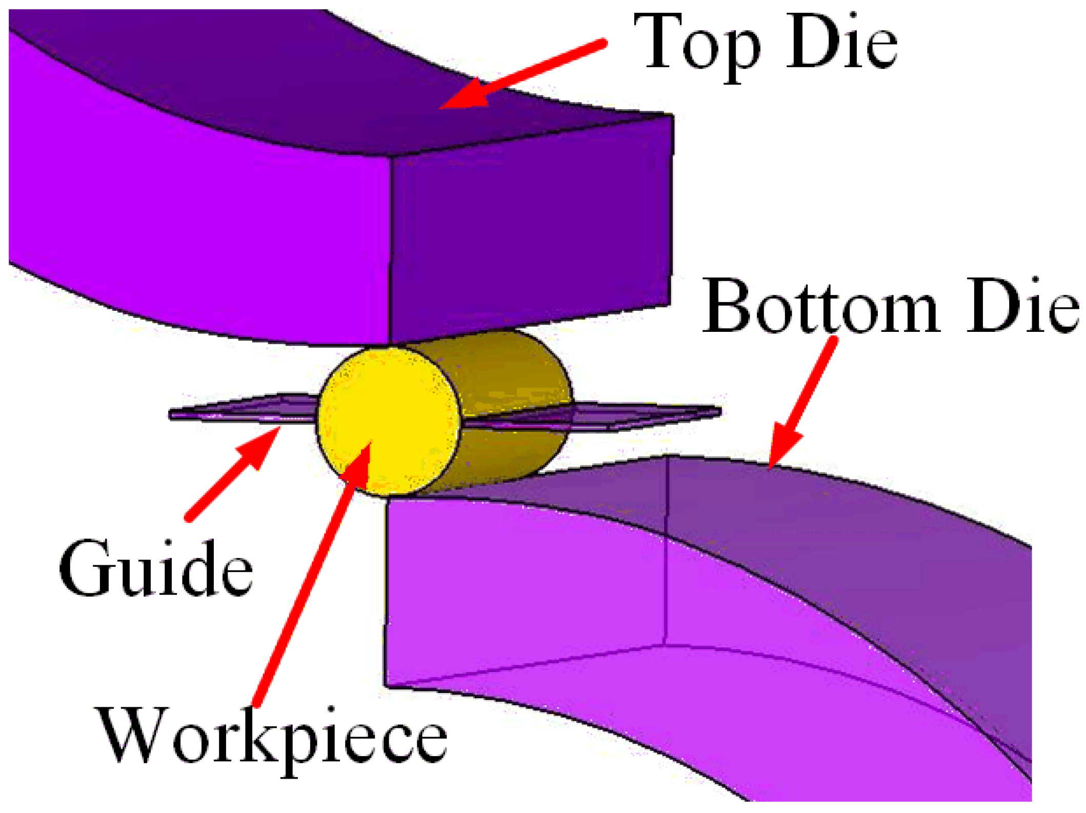
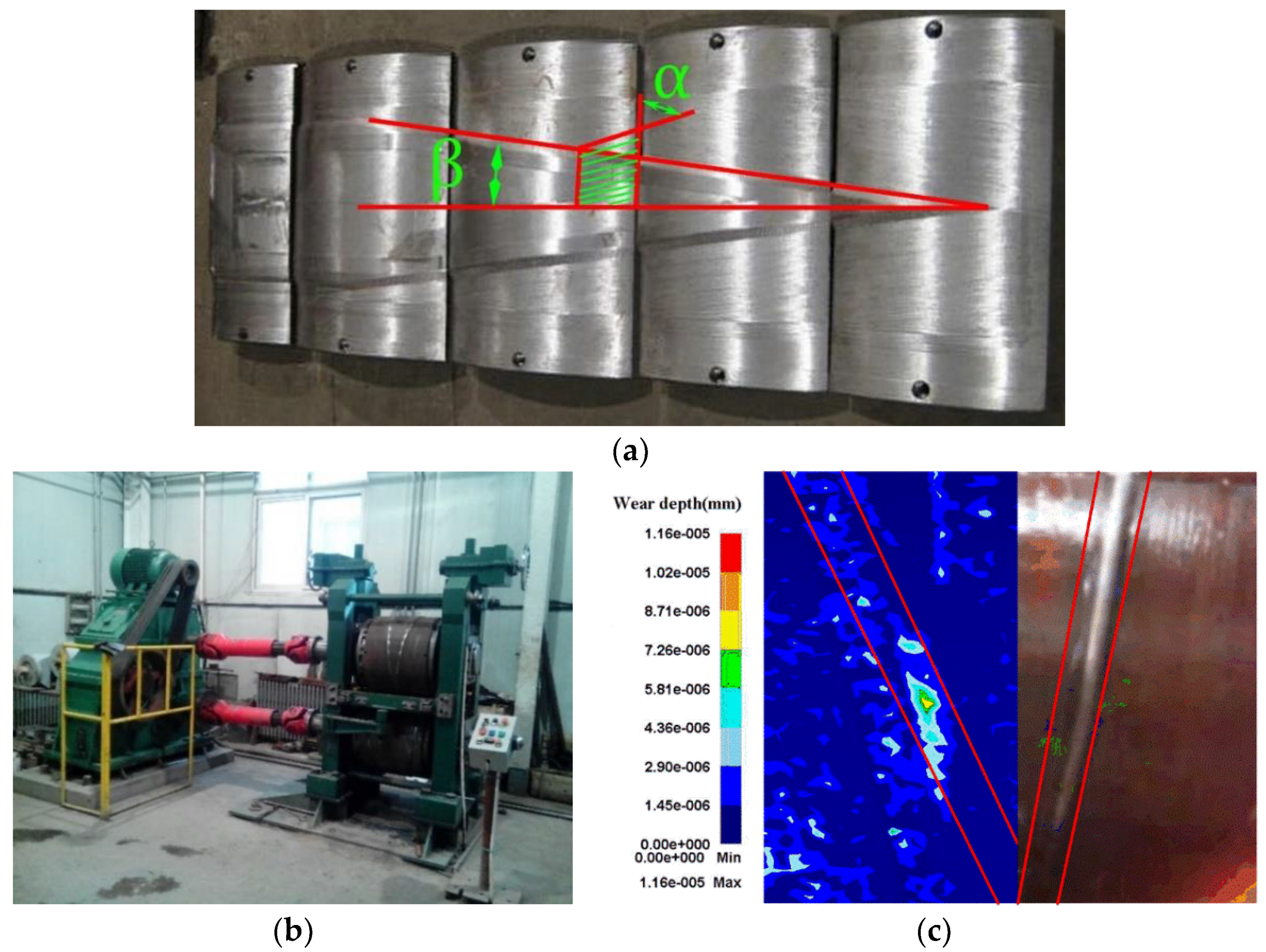
2.1. Geometric Parameters and Processing Conditions of the Mold
- (1)
- The Johson-Cook constitutive model [31] was established to predict the relationship between strain and stress of Ti-6Al-4V alloy at high temperature.
- (2)
- As shown in Figure 3a, load two restraint planes on both sides of the workpiece to keep the position of the workpiece stable.
- (3)
- Regard the mold and the guide plate as a rigid body and set the roller speed to be constant. In the actual rolling process, the roll speed will fluctuate at the beginning and the end of the rolling process. Roll speed is not considered in this study [32].
- (4)
- The friction model is set as the shear model, and the friction coefficient is set as a constant value. Tetrahedral finite element meshes are used in workpieces and abrasives. In addition, the method of refining mesh is adopted to improve the accuracy of simulation, as shown in Figure 3b.
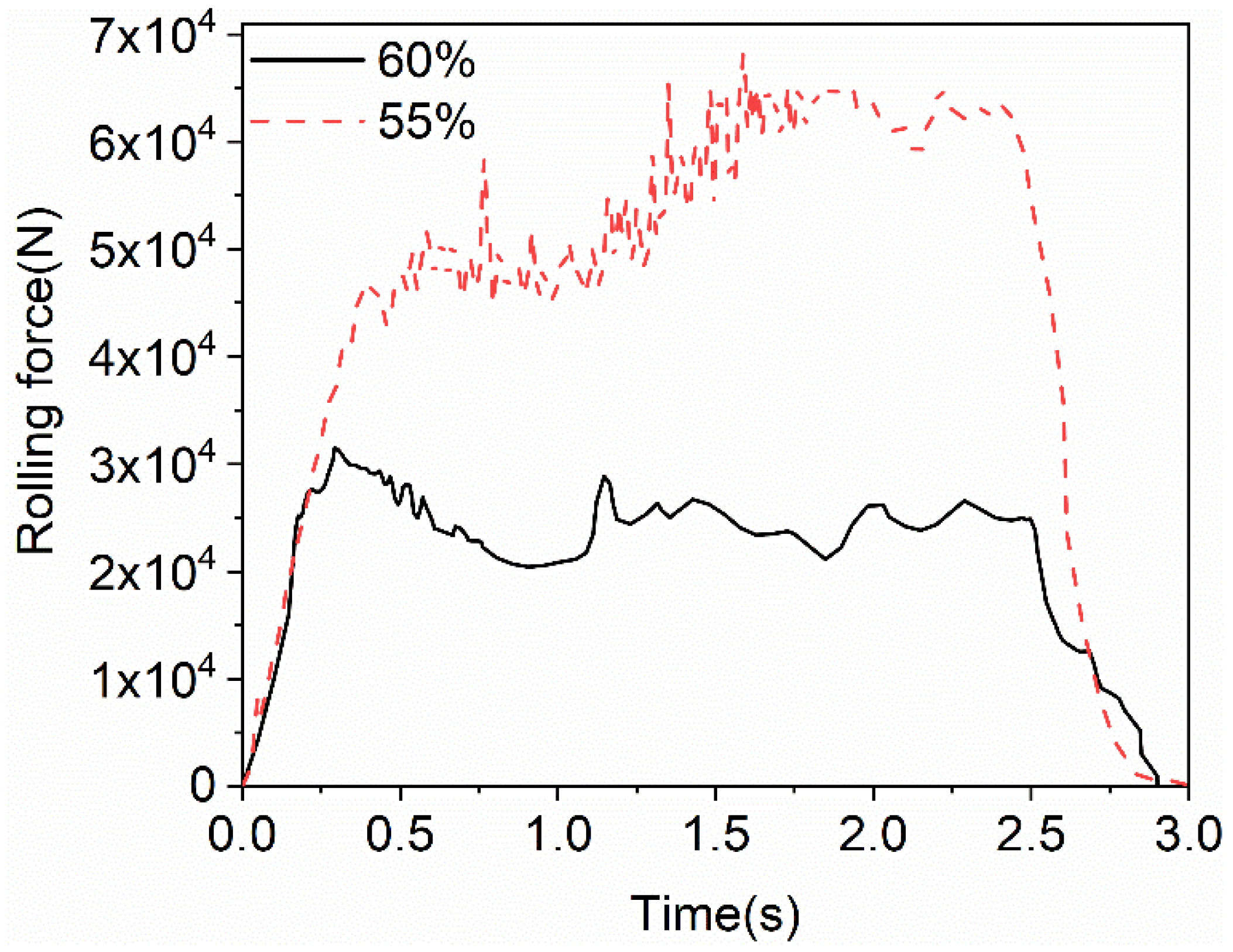
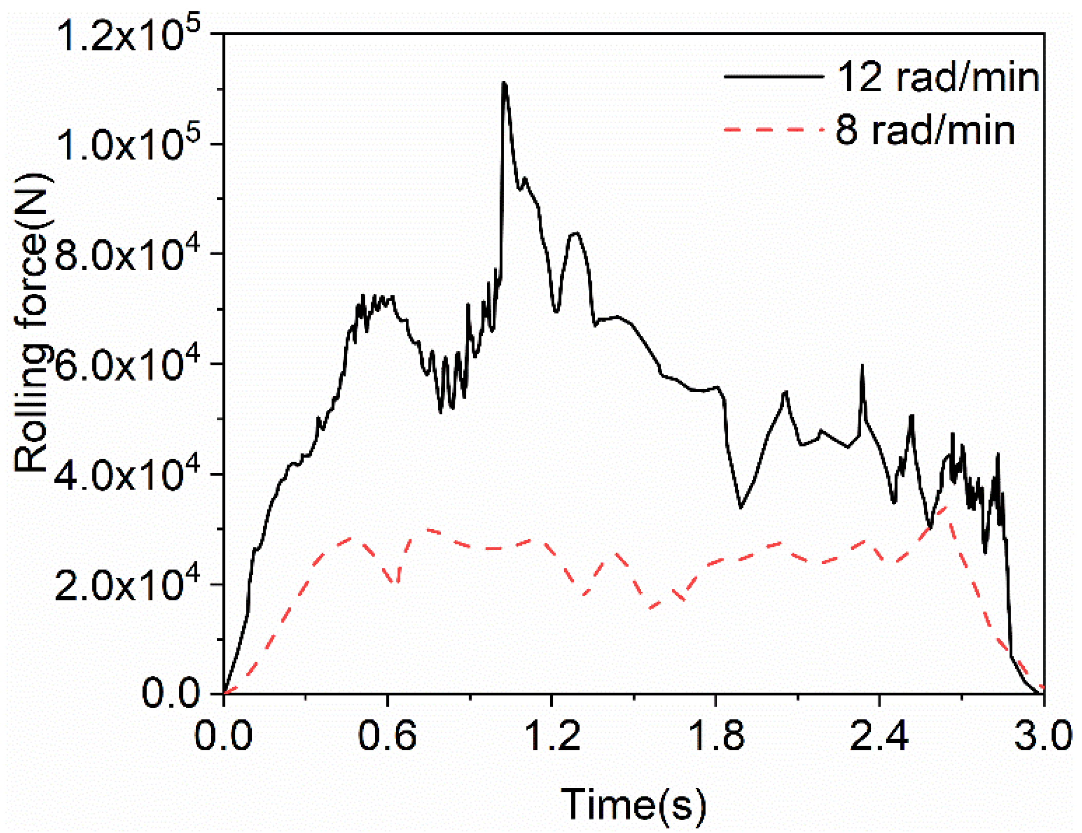
2.2. Orthogonal Test Design Based on Cross Wedge Rolling Process
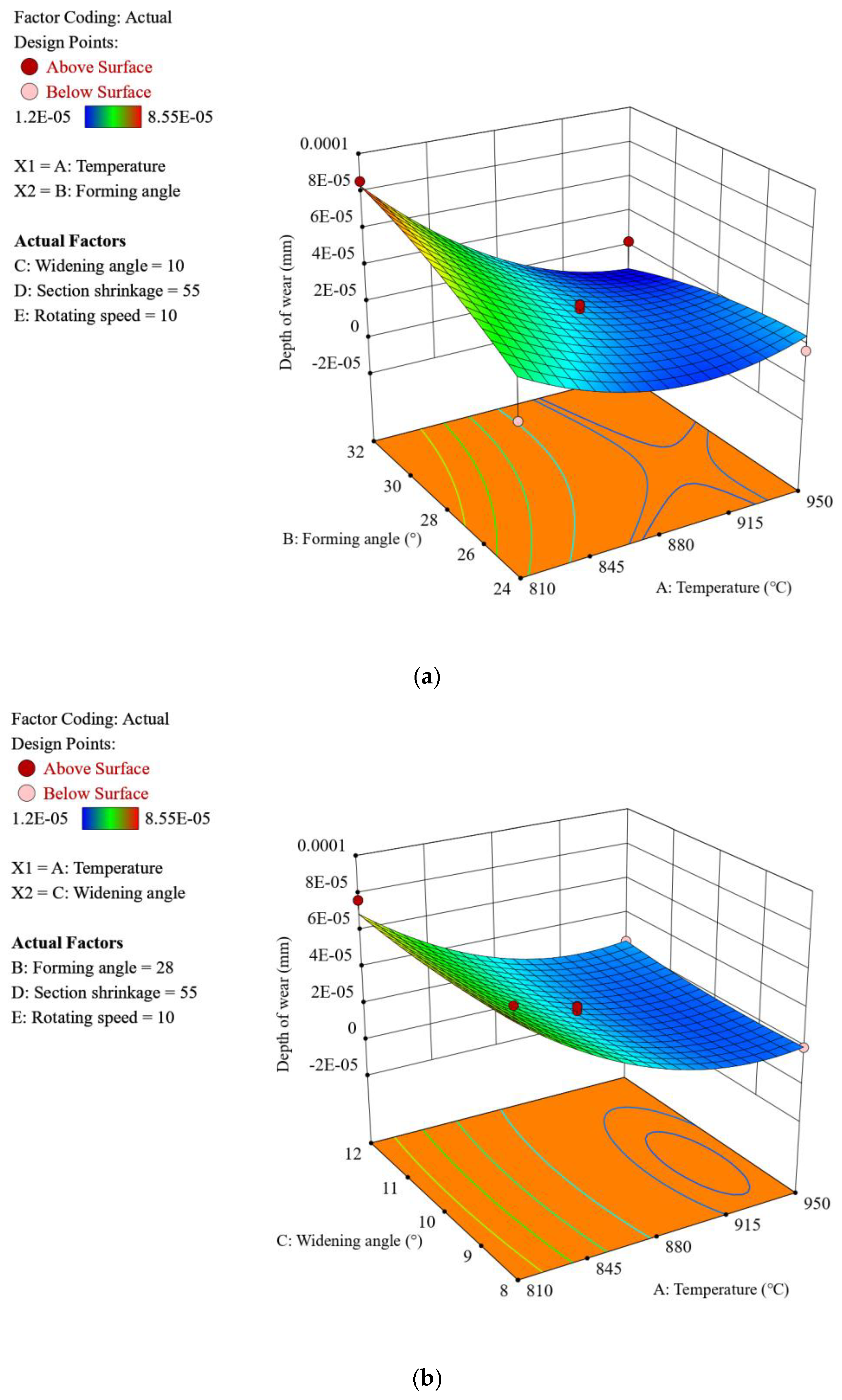
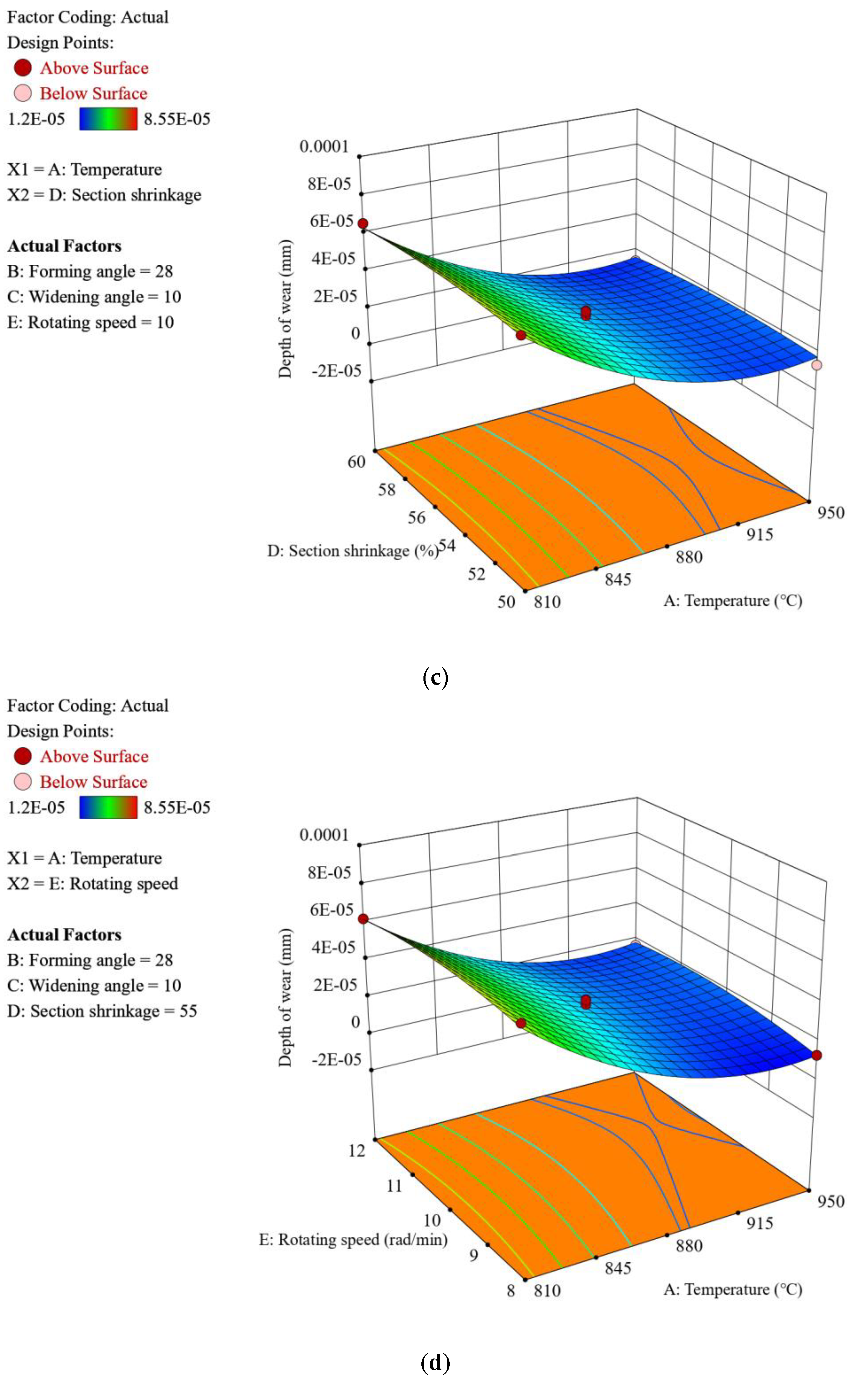
2.3. Response Surface Analysis
3. Parameter Optimization Based on BAS-GA-BP Model
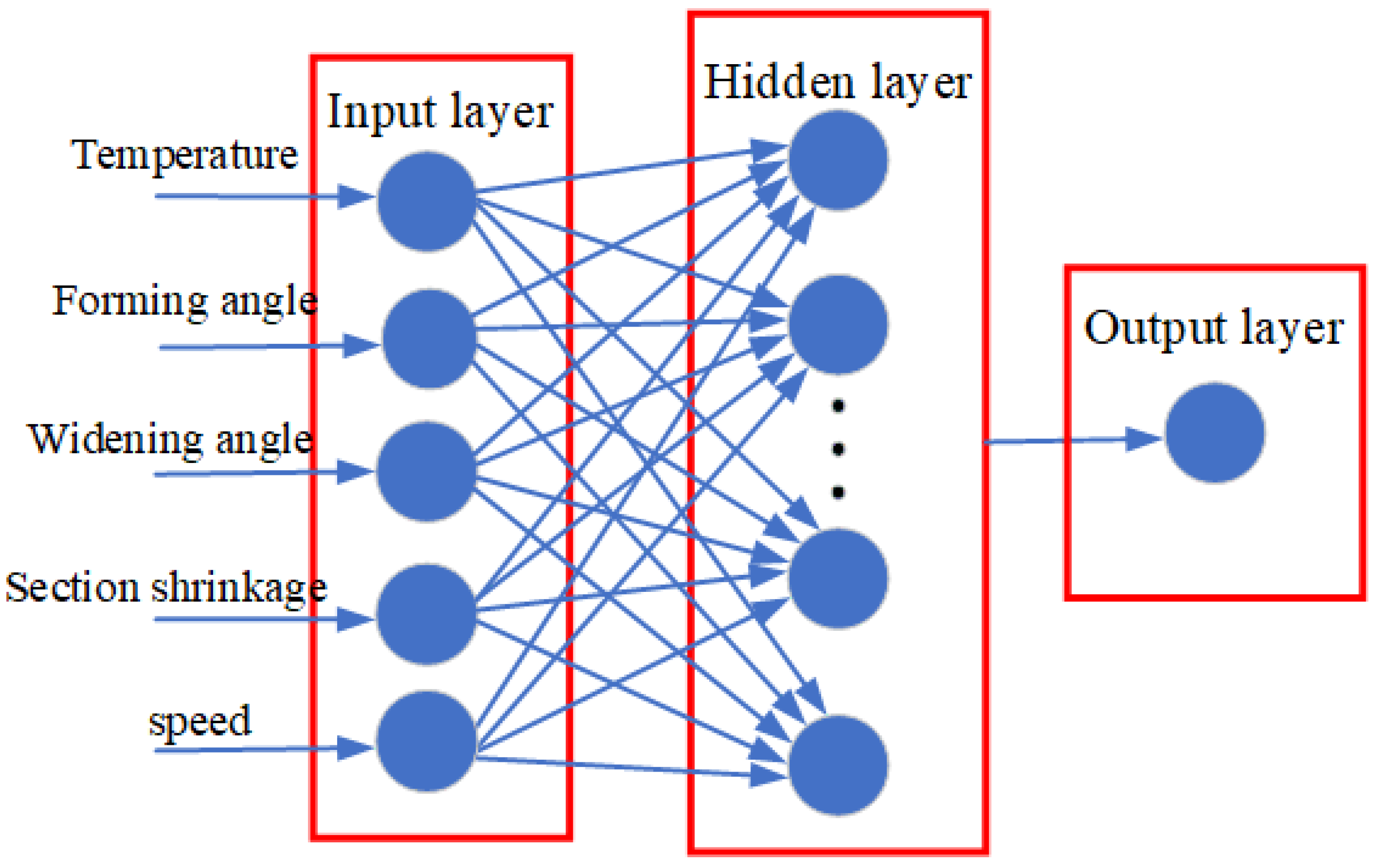
3.1. BP Neural Network Construction
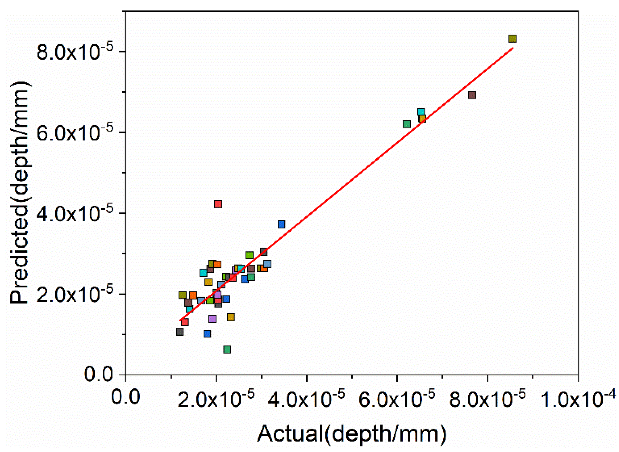
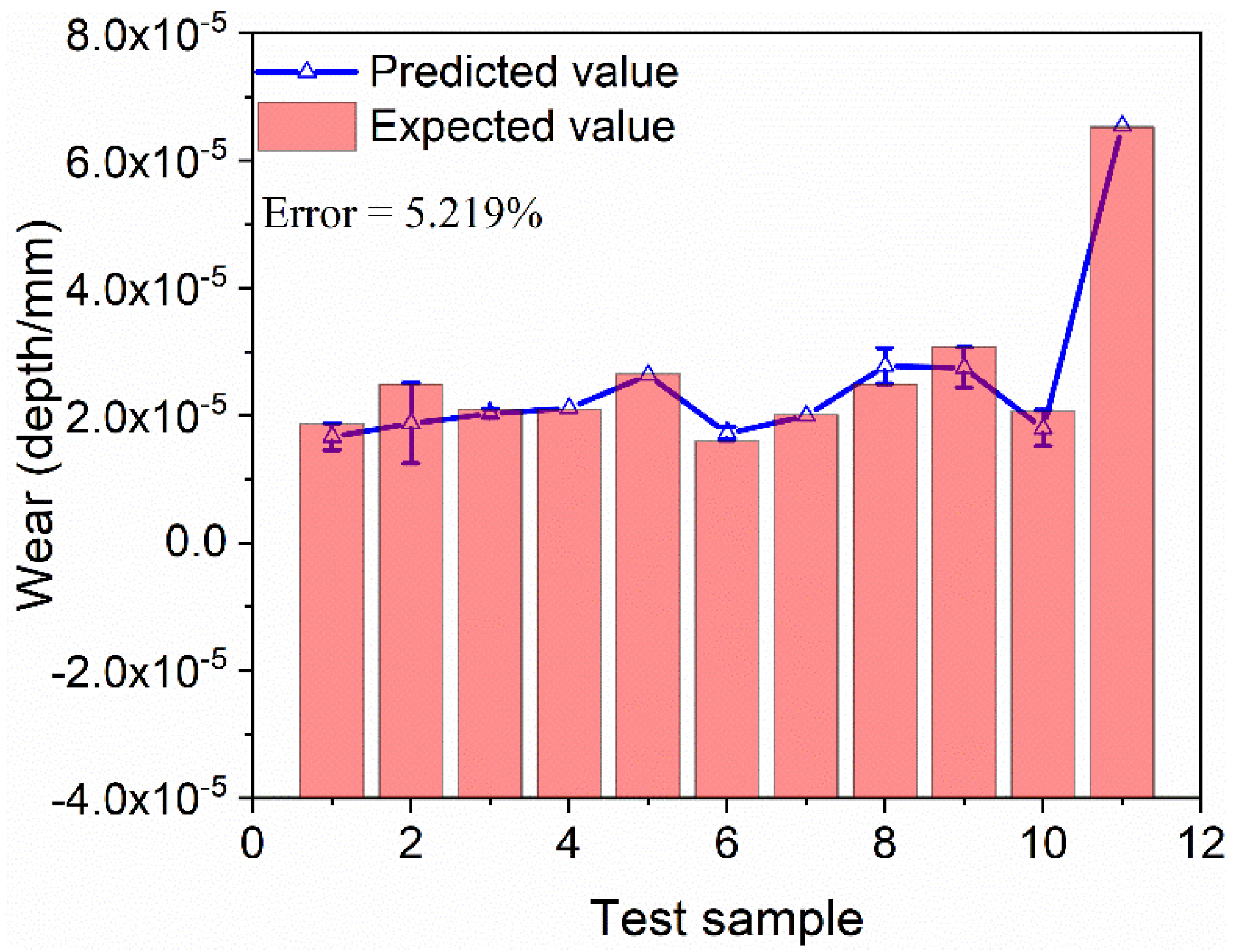
3.2. Goodness-of-Fit Test
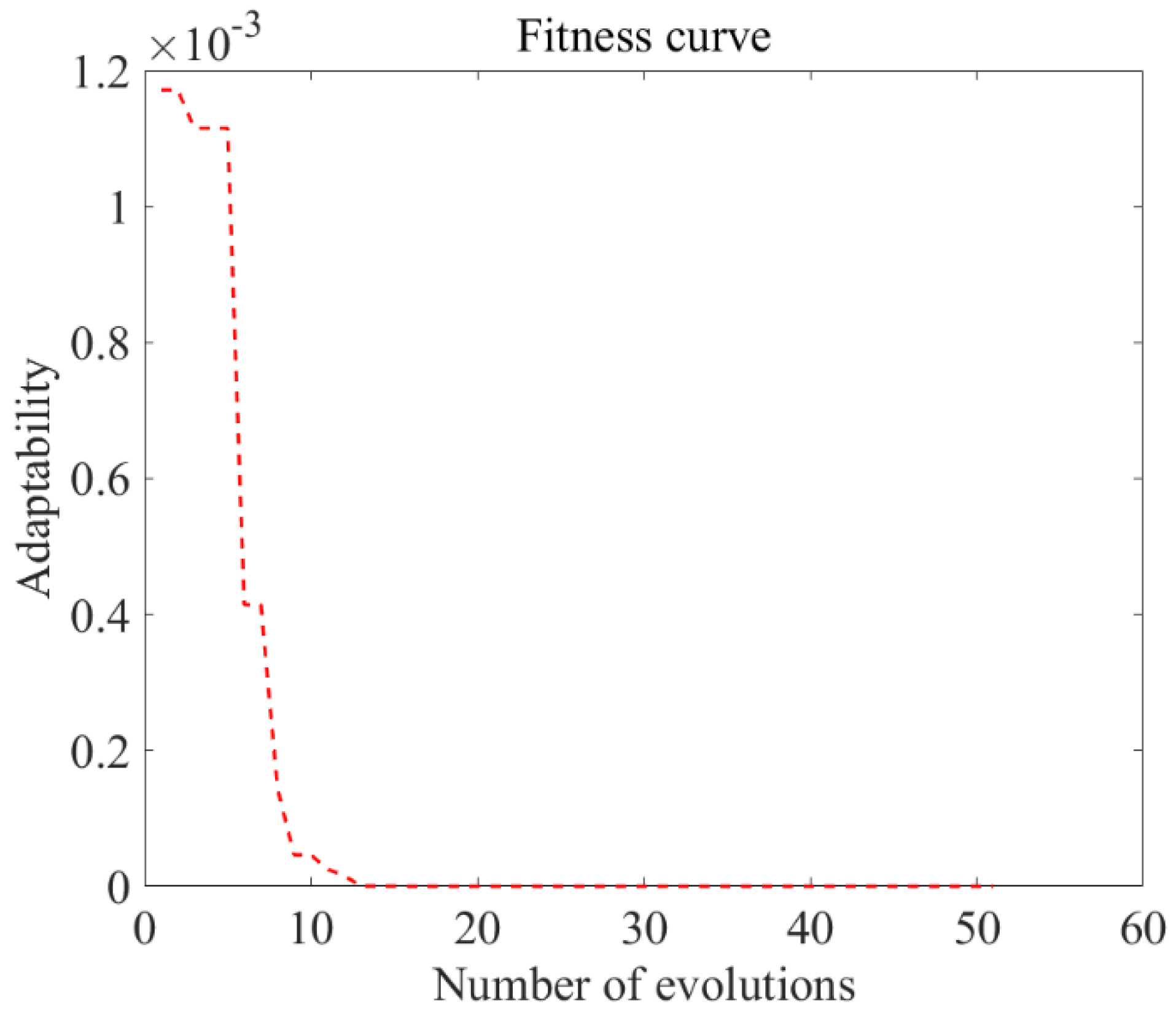
3.3. Establishment of BAS Algorithm
3.4. Simulation and Experimental Validation
4. Conclusions
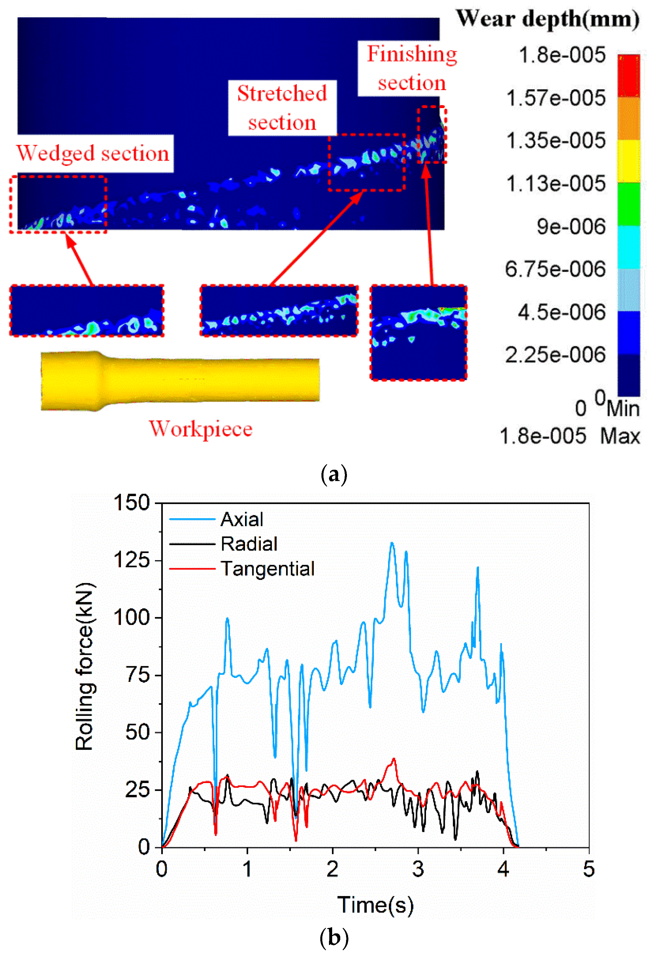
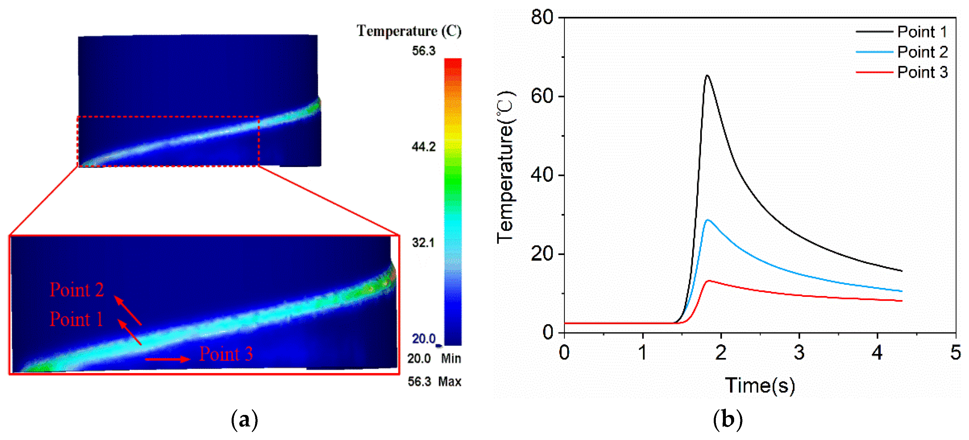
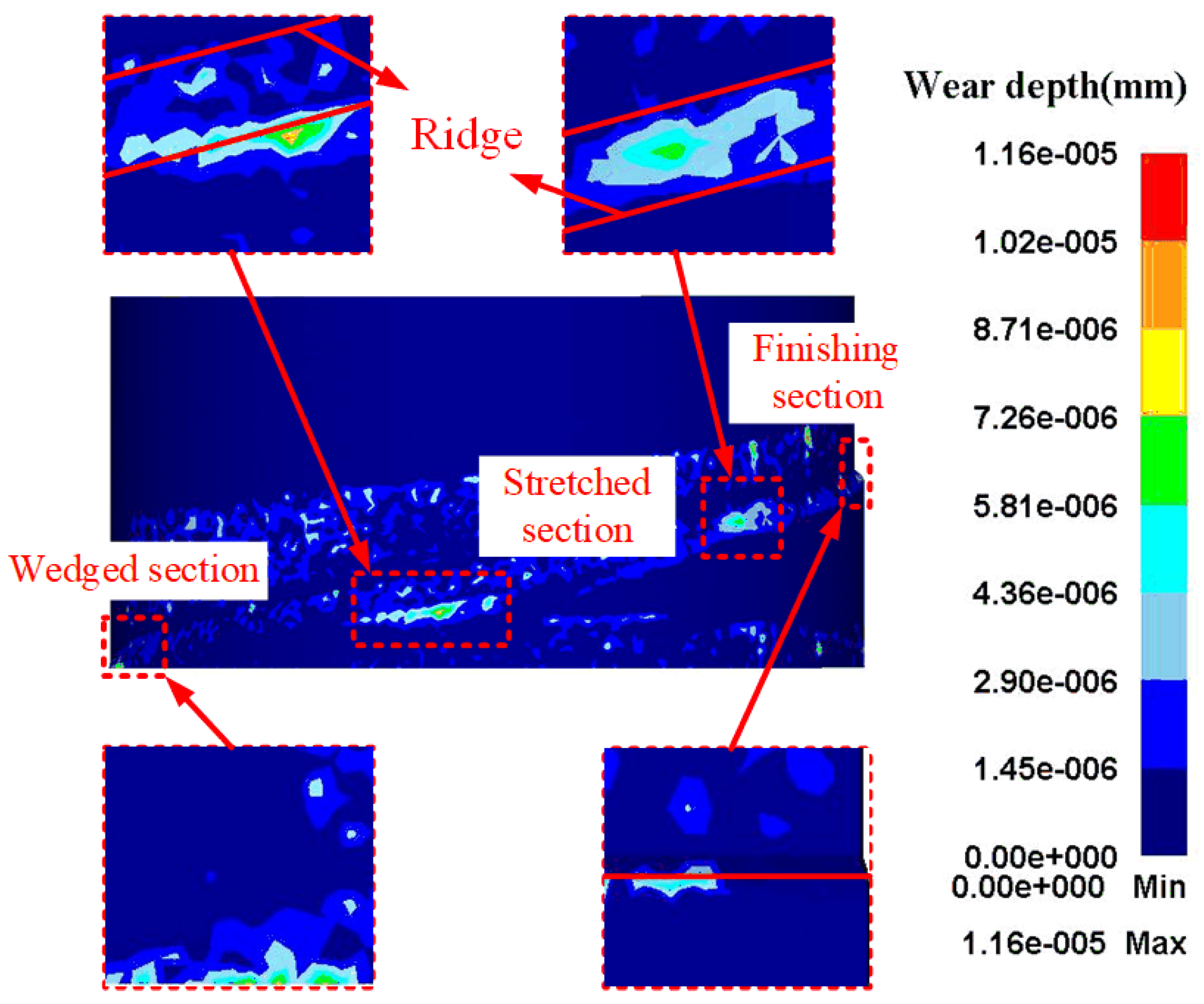
- Through finite element analysis, it is found that the area with the most serious wear on the die after rolling is basically concentrated on the inclined plane of wedges and the edge line of right angle. Wear depth is affected by the machining parameters, and the influence law is as follows: The wear depth increases with an increase in temperature and widening angle. It decreases with an increase in forming angle, section shrinkage, and rotating speed.
- A further conclusion is drawn through response surface analysis. Among all the deformation parameters, deformation temperature has the greatest influence on the wear depth of the die, followed by forming angle, while the other parameters have little effect on wear depth, and there is an interaction between forming angle and the deformation temperature.
- Through use of the GA-BAS-BP algorithm, the parameters that minimize the wear depth are obtained: T = 813.6845 °C; forming angle, 24.0674°; widening angle, 10.2415°; section shrinkage, 53.5077%; and rotating speed, 11.9768 rad/min. The wear value is 1.16 × 10⁻⁵ mm. The accuracy of the GA-BAS-BP algorithm is verified by comparison with the experiment.
Author Contributions
Funding
Data Availability Statement
Conflicts of Interest
References
- Huang, X.; Wang, B.; Mu, Y.; Shen, J.; Li, J.; Zhou, J. Investigation on the effect of mandrels on hollow shafts in cross-wedge rolling. Int. J. Adv. Manuf. Technol. 2019, 102, 443–455. [Google Scholar] [CrossRef]
- Zhu, S.; Peng, W.-F.; Shu, X.-D. Effect of tempering on bonding characteristics of cross wedge rolling 42CrMo/Q235 laminated shafts. J. Iron Steel Res. Int. 2020, 27, 1170–1178. [Google Scholar] [CrossRef]
- Pater, Z.; Tomczak, J.; Bulzak, T.; Walczuk-Gągała, P. Novel Damage Calibration Test Based on Cross-Wedge Rolling. J. Mater. Res. Technol. 2021, 13, 2016–2025. [Google Scholar] [CrossRef]
- Feng, P.; Yang, C.; Wang, B.; Li, J.; Shen, J.; Yang, X. Formability and microstructure of TC4 titanium alloy hollow shafts formed by cross-wedge rolling with a mandrel. Int. J. Adv. Manuf. Technol. 2021, 114, 365–377. [Google Scholar] [CrossRef]
- Meng, X.; Zhang, J.; Xiao, G.; Chen, Z.; Yi, M.; Xu, C. Tool wear prediction in milling based on a GSA-BP model with a multisensor fusion method. Int. J. Adv. Manuf. Technol. 2021, 114, 3793–3802. [Google Scholar] [CrossRef]
- Hisakado, T.; Miyazaki, K.; Kameta, A.; Negishi, S. Effects of surface roughness of roll metal pins on their friction and wear char-acteristics. Wear 2000, 239, 69–76. [Google Scholar] [CrossRef]
- Iwadoh, S.; Kuwamoto, H.; Sonoda, S. An Investigation about the Mechanism of Work Roll Wear at the Cold Rolling. Tetsu-to-Hagane 1989, 75, 2059–2066. [Google Scholar] [CrossRef] [Green Version]
- Luo, S.; Zhu, D.; Hua, L.; Qian, D.; Yan, S. Numerical analysis of die wear characteristics in hot forging of titanium alloy turbine blade. Int. J. Mech. Sci. 2017, 123, 260–270. [Google Scholar] [CrossRef]
- Riemer, O.; Elsner-Dörge, F. Investigation of material removal in vibration polishing of NiCo alloys with millimetre-sized tools. Int. J. Adv. Manuf. Technol. 2017, 92, 541–3122. [Google Scholar] [CrossRef]
- Shelke, R.D.; Rafiuddin, S.A. Numerical Simulation and Comparison of Carbide and HSS Tool Wear Rate while Drilling with Difficult to Cut Super Alloy Titanium Based on Archard Model. Int. J. Adv. Eng. Res. Sci. 2018, 5, 265244. [Google Scholar] [CrossRef] [Green Version]
- Kang, J.; Park, I.; Jae, J.; Kang, S. A study on a die wear model considering thermal softening: (I) Construction of the wear model. J. Mater. Process. Technol. 1999, 96, 53–58. [Google Scholar] [CrossRef]
- Behrens, B.-A. Finite element analysis of die wear in hot forging processes. CIRP Ann. 2008, 57, 305–308. [Google Scholar] [CrossRef]
- Lee, R.; Jou, J. Application of numerical simulation for wear analysis of warm forging die. J. Mater. Process. Technol. 2003, 140, 43–48. [Google Scholar] [CrossRef]
- Zhang, C.; Zhao, G.; Li, T.; Guan, Y.; Chen, H.; Li, P. An Investigation of Die Wear Behavior During Aluminum Alloy 7075 Tube Extrusion. J. Tribol. 2013, 135, 011602. [Google Scholar] [CrossRef]
- Hsu, Q.-C.; Do, A.T. Formation ability welding seams and mechanical properties of high strength alloy AA7075 when extrusion hollow square tube. Int. J. Precis. Eng. Manuf. 2015, 16, 557–566. [Google Scholar] [CrossRef]
- Huang, H.; Chen, X.; Fan, B.; Jin, Y.; Shu, X. Initial billet temperature influence and location investigation on tool wear in cross wedge rolling. Int. J. Adv. Manuf. Technol. 2015, 79, 1545–1556. [Google Scholar] [CrossRef]
- Hariprasad, T.; Shivalingappa, D.; Nagaraj, A.; Manivasagam, G. The use of artificial neural network for the prediction of wear loss of aluminium-magnesium alloys. Int. J. Comput. Aided Eng. Technol. 2015, 7, 72. [Google Scholar] [CrossRef]
- Huang, C.; Jia, X.; Zhang, Z. A Modified Back Propagation Artificial Neural Network Model Based on Genetic Algorithm to Predict the Flow Behavior of 5754 Aluminum Alloy. Materials 2018, 11, 855. [Google Scholar] [CrossRef] [Green Version]
- Syarif, J.; Detak, Y.P.; Ramli, R. Modeling of Correlation between Heat Treatment and Mechanical Properties of Ti–6Al–4V Alloy Using Feed Forward Back Propagation Neural Network. ISIJ Int. 2010, 50, 1689–1694. [Google Scholar] [CrossRef] [Green Version]
- Li, X.; Lu, H.; Wang, P. Parameters Optimization of γ-Ti-46.6Al-1.4Mn-2Mo Alloy by Hot-Pressing Sintering and its Micro-structures. Key Eng. Mater. 2013, 551, 92–99. [Google Scholar] [CrossRef]
- Jiang, X.; Li, S. BAS: Beetle Antennae Search Algorithm for Optimization Problems. Int. J. Robot. Control. 2018, 1, 1. [Google Scholar] [CrossRef]
- Jiang, X.; Li, S. Beetle antennae search without parameter tuning (BAS-WPT) for multi-objective optimization. Filomat 2020, 34, 5113–5119. [Google Scholar] [CrossRef]
- Archard, J.F. Contact and Rubbing of Flat Surfaces. J. Appl. Phys. 1953, 24, 981–988. [Google Scholar] [CrossRef]
- Snape, R.; Clift, S.; Bramley, A. Sensitivity of finite element analysis of forging to input parameters. J. Mater. Process. Technol. 1998, 82, 21–26. [Google Scholar] [CrossRef]
- Colás, R.; Ramírez, J.; Sandoval, I.; Morales, J.C.; Leduc, A.L. Damage in hot rolling work rolls. Wear 1999, 230, 56–60. [Google Scholar] [CrossRef]
- Xia, Y.; Shu, X.; Zhu, D.; Pater, Z.; Bartnicki, J. Effect of process parameters on microscopic uniformity of cross wedge rolling of GH4169 alloy shaft. J. Manuf. Process. 2021, 66, 145–152. [Google Scholar] [CrossRef]
- Sekine, Y.; Soyama, H. Evaluation of the surface of alloy tool steel treated by cavitation shotless peening using an eddy current method. Surf. Coat. Technol. 2009, 203, 2254–2259. [Google Scholar] [CrossRef]
- Kim, K.; Yang, H. Densification behavior of titanium alloy powder during hot pressing. Mater. Sci. Eng. A 2001, 313, 46–52. [Google Scholar] [CrossRef]
- Alimirzaloo, V.; Sadeghi, M.H.; Biglari, F.R. Optimization of the forging of aerofoil blade using the finite element method and fuzzy-Pareto based genetic algorithm. J. Mech. Sci. Technol. 2012, 26, 1801–1810. [Google Scholar] [CrossRef]
- Hu, H.-J.; Huang, W.-J. Studies on wears of ultrafine-grained ceramic tool and common ceramic tool during hard turning using Archard wear model. Int. J. Adv. Manuf. Technol. 2013, 69, 31–39. [Google Scholar] [CrossRef]
- Ji, H.; Peng, Z.; Pei, W.; Xin, L.; Ma, Z.; Lu, Y. Constitutive equation and hot processing map of TA15 titanium alloy. Mater. Res. Express 2020, 7, 046508. [Google Scholar] [CrossRef]
- Landgrebe, D.; Steger, J.; Böhmichen, U.; Bergmann, M. Modified Cross-Wedge Rolling for Creating Hollow Shafts. Procedia Manuf. 2018, 21, 53–59. [Google Scholar] [CrossRef]
- Jin, J.; Wang, X.; Deng, L.; Luo, J. A single-step hot stamping-forging process for aluminum alloy shell parts with nonuniform thickness. J. Mater. Process. Technol. 2016, 228, 170–178. [Google Scholar] [CrossRef]
- Ghani, J.; Choudhury, I.; Hassan, H. Application of Taguchi method in the optimization of end milling parameters. J. Mater. Process. Technol. 2004, 145, 84–92. [Google Scholar] [CrossRef]
- Sivapragash, M.; Kumaradhas, P.; Retnam, S.J.; Joseph, X.F.; Pillai, U. Taguchi based genetic approach for optimizing the PVD process parameter for coating ZrN on AZ91D magnesium alloy. Mater. Des. 2016, 90, 713–722. [Google Scholar] [CrossRef]
- Peng, W.-F.; Yan, C.; Zhang, X.; Shu, X.-D.; Huang, G.-X.; Xu, D.-M. Influence of process parameters on interfacial tensile strength of cross-wedge rolling of 42CrMo/Q235 laminated shafts. J. Iron Steel Res. Int. 2018, 25, 1003–1009. [Google Scholar] [CrossRef]
- Bulzak, T.; Pater, Z.; Tomczak, J.; Majerski, K. Hot and warm cross-wedge rolling of ball pins–Comparative analysis. J. Manuf. Process. 2019, 50, 90–101. [Google Scholar] [CrossRef]
- Peng, Z.; Ji, H.; Pei, W.; Liu, B.; Song, G. Constitutive relationship of TC4 titanium alloy based on back propagating (BP) neural network (NN). Metalurgija 2021, 60, 277–280. [Google Scholar]
- Song, C.D.; Kong, J.; Che, L. Prediction of TC16 Alloy Deformation Behavior Based on BP Neural Network. Adv. Mater. Res. 2013, 850–851, 96–101. [Google Scholar] [CrossRef]
- Guo, L.-F.; Li, B.-C.; Zhang, Z.-M. Constitutive relationship model of TC21 alloy based on artificial neural network. Trans. Nonferrous Met. Soc. China 2013, 23, 1761–1765. [Google Scholar] [CrossRef]
- Mandal, S.; Sivaprasad, P.; Venugopal, S.; Murthy, K.; Raj, B. Artificial neural network modeling of composition–process–property correlations in austenitic stainless steels. Mater. Sci. Eng. A 2008, 485, 571–580. [Google Scholar] [CrossRef]
- Schölkopf, B.; Platt, J.; Shawe-Taylor, J.; Smola, A.J.; Williamson, R.C. Estimating the Support of a High-Dimensional Distribution. Neural Comput. 2001, 13, 1443–1471. [Google Scholar] [CrossRef] [PubMed]


| Workpiece Ti-6Al-4V | Al | V | Fe | C | O | H | Ti | |
| 6.02 | 3.78 | 0.08 | 0.007 | 0.074 | 0.0082 | Bal. | ||
| Forging die H13 | Cr | V | Fe | C | Mo | Mn | Si | P |
| 2.08 | 0.84 | Bal. | 0.36 | 1.22 | 0.4 | 0.92 | 0.009 |
| Parameters | Forging Die | Workpiece |
|---|---|---|
| Material | SKD61 | Ti-6Al-4V |
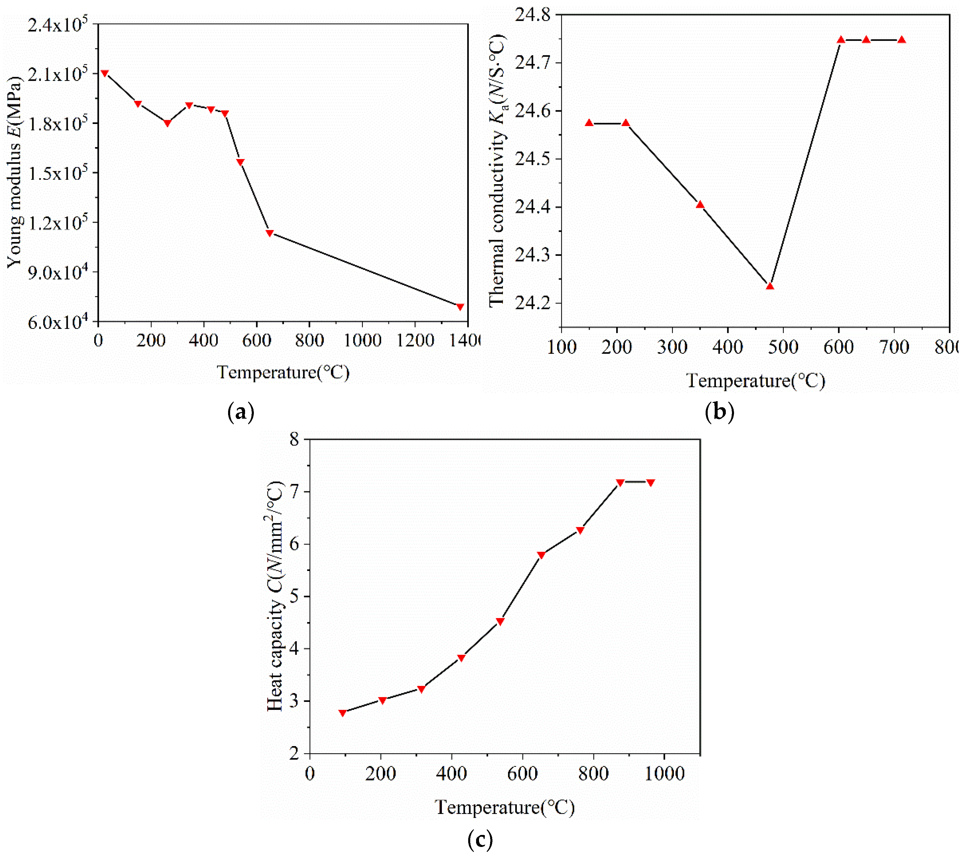
| Young’s modulus (MPa) | Figure 2a | Equation (7) |
| Poisson’s ratio | 0.3 | 0.342 |
| Density (Kg/mm3) | 7.8 × 10⁻⁶ | 4.43 × 10⁻⁶ |
| Thermal conductivity (N/(s °C)) | Figure 2b | Equation (8) |
| Heat capacity (N/(s mm2 °C)) | Figure 2c | Equation (9) |
| Emissivity | 0.7 [33] | 0.7 [29] |
| Convection coefficient to environment (N/(s mm °C)) | 0.02 | 0.02 |
| Heat transfer coefficient between workpiece and die (N/(s mm °C)) | 5 [29] | |
| Friction factor | 0.9 | |
| Initial temperature of workpiece (°C) | 810/880/950 | |
| Initial temperature of dies (°C) | 20 | |
| Environment temperature (°C) | 20 | |
| Step increment control(sec/step) | 0.05 | |
| Number of grids | 200,000 | 200,000 |
| Factor | Level 1 | Level 2 | Level 3 |
|---|---|---|---|
| Initial temperature of workpiece (°C) | 810 | 880 | 950 |
| Forming angle (°) | 24 | 28 | 32 |
| Widening angle (°) | 8 | 10 | 12 |
| Section shrinkage (%) | 40 | 50 | 60 |
| Rotating speed (rad·min−1) | 8 | 10 | 12 |
| Number | Temperature (°C) | Forming Angle (°) | Widening Angle (°) | Section Shrinkage (%) | Rotating Speed (rad·min−1) | Die-Wear Depth (mm) |
|---|---|---|---|---|---|---|
| 1 | 810 | 32 | 10 | 55 | 10 | 8.55 × 10⁻⁵ |
| 2 | 880 | 28 | 12 | 60 | 10 | 2.32 × 10⁻⁵ |
| 3 | 880 | 24 | 10 | 55 | 8 | 2.32 × 10⁻⁵ |
| 4 | 880 | 32 | 12 | 55 | 10 | 3.45 × 10⁻⁵ |
| 5 | 880 | 24 | 10 | 55 | 12 | 1.2 × 10⁻⁵ |
| 6 | 880 | 28 | 8 | 60 | 10 | 2.25 × 10⁻⁵ |
| 7 | 880 | 28 | 10 | 50 | 8 | 1.87 × 10⁻⁵ |
| 8 | 950 | 28 | 10 | 50 | 10 | 1.38 × 10⁻⁵ |
| 9 | 810 | 24 | 10 | 55 | 10 | 2.04 × 10⁻⁵ |
| 10 | 880 | 24 | 10 | 60 | 10 | 2.05 × 10⁻⁵ |
| 11 | 880 | 28 | 10 | 60 | 8 | 2.22 × 10⁻⁵ |
| 12 | 880 | 28 | 10 | 55 | 10 | 3.05 × 10⁻⁵ |
| 13 | 950 | 28 | 10 | 55 | 8 | 1.31 × 10⁻⁵ |
| 14 | 880 | 28 | 10 | 55 | 10 | 2.5 × 10⁻⁵ |
| 15 | 880 | 28 | 8 | 55 | 8 | 1.26 × 10⁻⁵ |
| 16 | 810 | 28 | 10 | 55 | 12 | 6.22 × 10⁻⁵ |
| 17 | 810 | 28 | 12 | 55 | 10 | 7.65 × 10⁻⁵ |
| 18 | 880 | 32 | 10 | 55 | 12 | 2.01 × 10⁻⁵ |
| 19 | 950 | 28 | 10 | 60 | 10 | 1.42 × 10⁻⁵ |
| 20 | 880 | 28 | 10 | 60 | 12 | 2.05 × 10⁻⁵ |
| 21 | 880 | 28 | 10 | 55 | 10 | 2.55 × 10⁻⁵ |
| 22 | 880 | 24 | 8 | 55 | 10 | 2.77 × 10⁻⁵ |
| 23 | 880 | 32 | 10 | 50 | 10 | 3.05 × 10⁻⁵ |
| 24 | 880 | 32 | 10 | 60 | 10 | 1.49 × 10⁻⁵ |
| 25 | 880 | 24 | 12 | 55 | 10 | 1.92 × 10⁻⁵ |
| 26 | 810 | 28 | 10 | 50 | 10 | 6.52 × 10⁻⁵ |
| 27 | 950 | 28 | 12 | 55 | 10 | 2.38 × 10⁻⁵ |
| 28 | 880 | 28 | 10 | 55 | 10 | 3 × 10⁻⁵ |
| 29 | 950 | 32 | 10 | 55 | 10 | 2.25 × 10⁻⁵ |
| 30 | 880 | 32 | 8 | 55 | 10 | 1.83 × 10⁻⁵ |
| 31 | 880 | 28 | 8 | 55 | 12 | 3.13 × 10⁻⁵ |
| 32 | 880 | 28 | 12 | 55 | 8 | 1.92 × 10⁻⁵ |
| 33 | 810 | 28 | 10 | 60 | 10 | 6.56 × 10⁻⁵ |
| 34 | 810 | 28 | 8 | 55 | 10 | 7.65 × 10⁻⁵ |
| 35 | 880 | 28 | 8 | 50 | 10 | 2.29 × 10⁻⁵ |
| 36 | 950 | 28 | 10 | 55 | 12 | 1.67 × 10⁻⁵ |
| 37 | 880 | 28 | 10 | 55 | 10 | 1.88 × 10⁻⁵ |
| 38 | 880 | 32 | 10 | 55 | 8 | 2.03 × 10⁻⁵ |
| 39 | 880 | 28 | 10 | 50 | 12 | 2.12 × 10⁻⁵ |
| 40 | 880 | 28 | 12 | 55 | 12 | 2.64 × 10⁻⁵ |
| 41 | 950 | 24 | 10 | 55 | 10 | 1.72 × 10⁻⁵ |
| 42 | 950 | 28 | 8 | 55 | 10 | 2 × 10⁻⁵ |
| 43 | 880 | 28 | 10 | 55 | 10 | 2.78 × 10⁻⁵ |
| 44 | 880 | 28 | 12 | 50 | 10 | 2.75 × 10⁻⁵ |
| 45 | 880 | 24 | 10 | 50 | 10 | 1.8 × 10⁻⁵ |
| 46 | 810 | 28 | 10 | 55 | 8 | 6.55 × 10⁻⁵ |
Publisher’s Note: MDPI stays neutral with regard to jurisdictional claims in published maps and institutional affiliations. |
© 2021 by the authors. Licensee MDPI, Basel, Switzerland. This article is an open access article distributed under the terms and conditions of the Creative Commons Attribution (CC BY) license (https://creativecommons.org/licenses/by/4.0/).
Share and Cite
Peng, Z.; Ji, H.; Huang, X.; Wang, B.; Xiao, W.; Wang, S. Numerical Analysis and Parameter Optimization of Wear Characteristics of Titanium Alloy Cross Wedge Rolling Die. Metals 2021, 11, 1998. https://doi.org/10.3390/met11121998
Peng Z, Ji H, Huang X, Wang B, Xiao W, Wang S. Numerical Analysis and Parameter Optimization of Wear Characteristics of Titanium Alloy Cross Wedge Rolling Die. Metals. 2021; 11(12):1998. https://doi.org/10.3390/met11121998
Chicago/Turabian StylePeng, Zhanshuo, Hongchao Ji, Xiaomin Huang, Baoyu Wang, Wenchao Xiao, and Shufu Wang. 2021. "Numerical Analysis and Parameter Optimization of Wear Characteristics of Titanium Alloy Cross Wedge Rolling Die" Metals 11, no. 12: 1998. https://doi.org/10.3390/met11121998