Abstract
The paper presents the comparison of optimization-regulation algorithms applied to the secondary cooling zone in continuous steel casting where the semi-product withdraws most of its thermal energy. In steel production, requirements towards obtaining defect-free semi-products are increasing day-by-day and the products, which would satisfy requirements of the consumers a few decades ago, are now far below the minimum required quality. To fulfill the quality demands towards minimum occurrence of defects in secondary cooling as possible, some regulation in the casting process is needed. The main concept of this paper is to analyze and compare the most known metaheuristic optimization approaches applied to the continuous steel casting process. Heat transfer and solidification phenomena are solved by using a fast 2.5D slice numerical model. The objective function is set to minimize the surface temperature differences in secondary cooling zones between calculated and targeted surface temperatures by suitable water flow rates through cooling nozzles. Obtained optimization results are discussed and the most suitable algorithm for this type of optimization problem is identified. Temperature deviations and cooling water flow rates in the secondary cooling zone, together with convergence rate and operation times needed to reach the stop criterium for each optimization approach, are analyzed and compared to target casting conditions based on a required temperature distribution of the strand. The paper also contains a brief description of applied heuristic algorithms. Some of the algorithms exhibited faster convergence rate than others, but the optimal solution was reached in every optimization run by only one algorithm.
1. Introduction
The use of the continuous steel casting process has been experiencing a constant growth since the 1950s, when the ingot casting was replaced by the new method, which could satisfy increasing demands towards higher steel quality and production rate. Since those days, the continuous casting (CC) method evolved to a dominant steel production process. To avoid casting of semi-products with defects such as cracks, the casting regulation in real time is a necessity. Heat withdrawal from the strand can be now controlled by mathematical numerical models, even the real-time decisions during the casting process can be made owing to sophisticated code structure [1].
The CC of steel can be done with horizontal, vertical, or radial continuous casting machines (CCMs). The last-mentioned machine is the most used type worldwide as it overcomes the drawbacks of the other two machines [2]. That is the reason why the radial CC is also considered in this study. The CCM (see Figure 1) is a complex machine composed of many parts, which are usually divided to sections of the primary cooling zone (mold), the secondary cooling zone (water-air nozzle cooling), the tertiary cooling zone (radiation only with no nozzles), the cutting section and the chill zone where the cast semi-products (billet, bloom, slab, etc.) rest until they are further proceeded. Some of these parts contribute to the heat withdrawal from a strand and these must be implemented in the numerical heat transfer and solidification model. As the process is transient, the initial and boundary conditions need to be specified for a precise prediction of the heat withdrawal and the temperature distribution. In the primary cooling zone referred to as the mold, heat transfer is governed mainly by heat conduction across the interfacial gap between the strand and the mold wall. In the secondary cooling zone, the most challenging task is to precisely describe heat transfer and its phenomena, including water-spray cooling, droplets impingement to the surface of the strand and liquid film boiling that may occur at the strand surface.
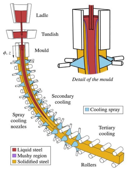
Figure 1.
Radial continuous casting machine (CCM) depicting primary, secondary and tertiary cooling zones [3] (with the permission of Elsevier).
The main objective of this paper is to investigate and compare some of the well-known heuristic approaches coupled with a solidification model in terms of the computational efficiency, robustness, and accuracy to the CC problem. This approach makes it possible to appropriately assess the efficiency and accuracy of individual optimization algorithms, reducing a direct influence of the heat transfer and solidification model of the CC since the model is identical in all considered cases with distinct optimization algorithms. According to the literature survey focusing on minimization of the occurrence of defects in CC (mainly defects in secondary cooling), the target strand surface temperatures along the caster were set in this respect. The optimization problem was formulated to find adequate cooling intensities (water flow rates in secondary cooling) for all the cooling nozzles in order to reach specified ranges of the target surface temperature.
1.1. Conditions towards High-Quality Steel Casting
A crucial question is how to maximize the steel quality and productivity with the minimal cost. One of the main causes of crack formation is the exceeding maximum allowable mechanical strain and stress, which the cast steel grade can withstand. A literature survey on metallurgical problems and crack formations in continuous steel casting affecting the quality of steel, particularly in the secondary cooling zone, is presented below. Some of these properties can be implemented to the solidification thermal model, but to evaluate all of them, the stress-strain, fluid flow, segregation models and their coupling need to be considered [1]. Brimacombe [4] summarized fundamentals of steel and identified different types of cracks. The knowledge base about the high-quality casting was set. The serious problem in CC—the breakout of the liquid steel below the mold—can be initialized with a too high temperature of the liquid steel in the tundish [5]. As a result, the mold does not provide a sufficient cooling rate to create the necessary solidified shell at the surface of the strand. Nevertheless, if the shell would withstand the hydrostatic pressure of the liquid steel, the whole casting would be shifted in terms of the optimal temperature intervals along the CCM this would also affects the steel quality of the strand. Moreover, the origin of cracks caused by bending and straightening (unbending) processes is also influenced by the temperature-dependent ductility of steel [6].
The crack formation including centerline, intermediate, triangle, midway cracks, etc. is particularly triggered by an improper setup of primary and secondary cooling intensities, excessive oscillation of the mold and excessive gaps between supporting rollers, especially in slab casting [7]. The most frequent surface defects are transversal cracks, which are particularly initialized by deep oscillation marks followed by the tension generated by bulging, bending, and straightening of the strand. Another cause for developing mechanical strain can be poor accuracy of arcing between the segments and abnormal roll-gap shrinkage, which leads to excessive bulging. There is also an influence of the thermal stress, which results from an uneven cooling of the strand shell in the secondary cooling zone. Kulkarni and Babu [8] considered coupled thermal and mechanical conditions and proposed 17 quality criteria, which allow for the reduction of occurrence of defects during the casting process. This approach of optimization needs both thermal and mechanical models to be coupled. From studies of Cheung et al. and Kong et al. [9,10], it is known that the temperature regeneration between cooling sections should be less than 150 °C to avoid stress due to bulging and reheating in the secondary cooling zone. Reheating beyond 150 °C/m leads to a high probability of forming intermediate cracks. Surface cracks are formed if the surface temperature decreases into a zone of low steel ductility, which depends on steel grade; Santos et al. [11] identified it as being under around 850 °C. Cheung et al. [12] discussed the formation of cracks in steel casting and contributed to high-quality casting knowledge base with other optimal casting conditions. The authors discussed the centerline segregation and its impact to the crack formation while the centerline of the strand was liquid in the unbending part and pointed out that the center solidification of the strand must be completed before the point where a high deformation is applied (unbending point).
Brimacombe and Sorimachi [6] documented that the steel has reduced ductility over specific temperature ranges (Figure 2) dependent on the steel composition, which has important implications for the crack formation. Kim et al. [13] mentioned the so-called reduced ductility regions, namely zero ductility temperatures (ZDTs) and liquid impenetrable temperatures (LITs). Internal cracks detected in strands mainly originate in the mushy zone where the solid fraction of steel reaches 0.9 and 0.99 value for the LITs and ZDTs, respectively. These LIT and ZDT zones are sensitive for cracking because the steel is brittle in these temperature zones and has a higher tendency to hot cracking, and thus, it has a higher tendency towards the creation of defects [14]. The problem of crack formation in these locations is that the dendrite arms are dense enough to prevent the liquid steel to fill in gaps [15]. A lower solidification temperature is observed in these areas, which is a consequence of micro-segregation, and together with the shrinkage, the steel is more prone to cracking while the tensile stress can reach lower values and cause cracking. The LITs and ZDTs are functions of chemical compositions and vary for different steel grades. Steel grades with larger temperature differences between the LIT and ZDT have a higher tendency to hot cracking and thus have a higher tendency to form defects such as internal cracks in the CC.
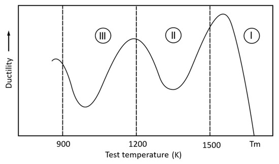
Figure 2.
Schematic representation of temperature regions with reduced ductility redrawn from [16] (with the permission of Elsevier). For further details, see [16].
1.2. Numerical Modeling of Thermal Behavior in CC
In the steel CC, many numerical models have been used since the computational technique developed significantly. In the available literature, a number of implementations using the finite difference, finite volume or finite element methods can be found. In some previous works (e.g., by Fic et al. [17]), models with rather unrealistic assumptions of steel undergoing the phase change at a constant temperature were considered. The user-friendly packages that can predict variable-dependent thermophysical and mechanical properties were introduced in [18,19] and enabled more accurate modelling. Meng and Thomas [20] developed a 1D transient heat transfer model of the strand coupled with a 2D steady-state heat transfer model of the mold. Metallurgical phenomena such as the slag behavior in the mold and effects of oscillation marks were examined. Alizadeh et al. [21] proposed a 2D model and observed that the casting speed is the most effective parameter to heat removal in the mold, which means that it is the most important factor in control of the solidified shell thickness and strand temperature. Hardin et al. [22] presented a parametric study on more advanced transient 2D model, which allowed to observe the temperature response on the casting speed changes. One of the first 3D solidification model was introduced by Tieu and Kim [23] in 1997. The part of their work points to advantages of the 3D approach in comparison to 2D models. Another approach towards 3D heat transfer in the CC process is to use the so-called slice model, which neglects the heat transfer by conduction in the casting direction. This type of the solidification model is presented, for example, by Tambunan [24].
Due to limitations in terms of the computational performance, these models are often simplified: They use a simple geometry, constant thermophysical properties, average boundary conditions, use of empirical formulas for heat removal in the mold and secondary cooling, simulate only one quarter of the strand cross-section, etc. However, computational capabilities have progressed to the point where models used in the CC control include only minor physical simplifications, can provide more accurate results and can be used for steel quality optimization in real processing time. Utilizing the GPU-based model [3] enabled to overstep large numbers of shortcomings and resulted in a significantly reduced computing time while compared to CPU-based models.
1.3. Optimization and Regulation Algorithms in CC
To reach the optimal temperature intervals for a particular grade of steel and to react to dynamical changes such as an abrupt change of the casting speed, the solidification model must be coupled with optimization and control algorithms. One-dimensional mold cooling optimizations were among the very first optimization approaches which examined break outs at the mold exit due to the inappropriate shell thickness. During the two decades of the twenty-first century, computational techniques and performance experienced an exponential increase and simulation results can be obtained in the fraction of time that was needed two decades ago. This allowed many optimization algorithms to develop and get into practice. There are many papers which combine numerical modelling and optimization-regulation approaches in CC, such as Santos et al. [11], who applied the genetic algorithm and determined the optimum settings of water flow rates in different sprays zones. Optimized cooling conditions of mold and secondary cooling zones resulted in a shorter metallurgical length with the same quality [9]. Ji et al. [25] verified the use of the ant colony algorithm and Zheng et al. [26] used swarm optimization. Rao et al. [27] published a comprehensive review dealing with parameter-based optimization of selected casting processes. The authors pointed out that various optimization techniques such as simulated annealing [28], genetic algorithm [29] and particle swarm optimization [30] applied to the CC process does not always find the optimal solution. To control the casting process, these supervision systems include regulation algorithms such as the PID regulation which exhibit a slower response against a very fast regulation using fuzzy logic [31]. Mauder et al. in [31] introduced a 3D fully-transient and advanced optimal control algorithm based on the fuzzy logic that enabled a smooth regulation of cooling nozzles to the casting speed change.
Unfortunately, these works often needed a large number of optimization iterations before the optimal solution was found. It is; therefore, impossible to compare these approaches to each other since every author used his/her own specific solidification model and other specific conditions and setup. This drawback was the motivation for the present paper. In this paper, five optimization algorithms and their performance applied to the optimization of the CC are compared in terms of the heuristic search of appropriate water flow rates through cooling nozzles to reach the target temperature distribution of the strand, which would satisfy requirements towards a higher steel quality.
2. Slice Solidification Model
The mathematical formulation of heat transfer and solidification to the temperature distribution and solid shell profile prediction is based on the governing equation of transient heat conduction, called the Fourier-Kirchhoff equation [32]. To decrease the computational time in solving the optimization problem requiring a large number of evaluations of the model with various casting parameters, the 3D Fourier-Kirchhoff equation can be reformulated for the so-called 2.5D moving slice model neglecting conduction heat transfer in the casting direction (z). The heat transfer equation for the 2.5D slice model formulated with the enthalpy approach reads
where keff is the effective thermal conductivity (W·m−1·K−1), T is the temperature (K), H is the volume enthalpy (J m−3), t is the time (s) and x, y, and z are spatial coordinates. Fluid flow of the liquid steel can be calculated by the computational fluid dynamics (CFD) techniques. However, computational time of such simulations is too excessive for real-time applications. The influence of fluid flow can be accounted in a simplified way by means of the effective thermal conductivity keff. Increasing heat transfer due to convection in the flow of liquid steel at different distances from the meniscus can be considered by an increased effective thermal conductivity as proposed by Zhang et al. [33]. For more information about the solidification model in terms of equations, initial and boundary conditions, see the previous works of the co-authors of this paper [3,31].
The advantage of the model applied in this paper, when compared to models using empirical formulas for the heat transfer coefficient under the water-air cooling nozzles, is the use of experimentally measured characteristics of all nozzles used at the caster. As a result of many years of experience with computational inverse heat transfer in the heat transfer and fluid flow laboratory at Brno University of Technology, the heat transfer coefficient characteristics of nozzles can be experimentally determined with the use of a so-called hot plate and used in solidification numerical models [34]. In general, the heat transfer coefficient (htc) of each nozzle is determined as a function of the casting speed, water mass flow rate, air pressure and the surface temperature and it can be expressed as
The purpose of the slice model is to provide a thermo-solidification 2.5D analysis for a slice perpendicular to the longitudinal strand axis, see Figure 3. The whole casting strand (in this paper, the length from the meniscus to the cutting torch is considered 27.2 m) is divided into a number of slices having a defined thickness. In this paper, it was decided to set the slice thickness to 25 mm. The thickness of the slice needs to be chosen properly to achieve a sufficient precision of the boundary conditions describing heat withdrawal from the strand. The initial slice starts at the meniscus in the mold and moves downwards through the whole caster until it reaches the cutting part of the CCM. The explicit finite difference method was used in the thermal numerical model. Thus, the maximum numerical time step had to be defined to avoid numerical oscillations in the explicit calculation. The time step of the explicit scheme needs to be smaller than the wall-clock time required by the slice for its movement to the following position in the casting direction. The required time to move the slice to the following position was determined as a ratio between the thickness of the slice and the casting speed. New temperature field of the moving slice is initially set to the final temperature field of the previous slice and the boundary conditions corresponding to the slice location are applied for the evaluation of heat transfer. This type of 2.5D slice model significantly reduces the computational time in contrast to the fully 3D model, where the complete temperature distribution of the strand is calculated in each time step.
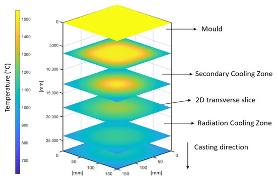
Figure 3.
Idea of the 2.5D slice model.
Thermophysical Properties
A low-carbon steel grade 18CrNiMo7-6 and a billet having the cross-section of 150 mm × 150 mm were considered in this paper. The thermophysical properties of the steel grade were determined in the temperature range from 1600 °C to the room temperature by means of the solidification analysis package IDS (version 1.3.1, created at Helsinki University of Technology, Laboratory of Metallurgy) [19] The temperature-dependent enthalpy and other thermophysical properties (density, specific heat, thermal conductivity) identified with the IDS for the steel grade 18CrNiMo7-6 are shown in Figure 4.
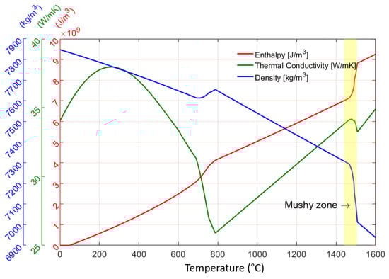
Figure 4.
Thermophysical properties of structural steel 18CrNiMo7-6.
3. Optimization Approach
The 2.5D slice solidification model predicts the temperature distribution of the strand under certain values of the casting parameters, such as the casting speed, heat withdrawal in the mold, the secondary cooling intensity, etc. The problem is how to set these input parameters in a way to get a high-quality steel with a minimum occurrence of defects. This is referred to as an inverse problem and, to solve this issue, optimization algorithms need to be used. The solidification model is based on the discretization of Equation (1), which generally leads to millions of nonlinear finite-difference equations. A direct optimization approach with mathematical programming methods is not applicable, as the computational complexity and computation time grow exponentially with the size of the numerical mesh. Thus, it is needed to separate the optimization algorithm and the solidification model, which is referred to as the so-called black-box approach. In this approach, the optimization algorithm controls input parameters (speed of casting, intensity of water spray cooling, etc.) to the solidification model. The solidification model predicts the temperature distribution under the particular casting parameters and provides it to the optimization algorithm. Based on the temperature distribution, the optimization algorithm evaluates the objective function, somehow modifies input casting parameters and repeats the described process in a closed loop until the optimal solution is found. The computational efficiency of the optimization algorithm is usually assessed from the viewpoint of the number of iterations, which the algorithm needs to reach the optimal solution [35].
To deal with complex computational problems such as the CC, some optimization algorithms have been inspired by biological mechanisms in the nature. The nature acts as a source of concepts and principles for designing artificial computing systems [36]. So-called nature-inspired meta-heuristic algorithms attempt to solve optimization problems by mimicking biological or physical phenomena. Meta-heuristics can be grouped in four main categories based on the applied techniques, population and convergence logic used to reach the optimal solution (see Figure 5): evolution-based, physics-based, swarm-based and human-based methods [37]. Laws of the natural evolution inspired the evolutionary-based methods. A randomly generated population starts the optimization process and evolves over subsequent generations with the combination of the best individuals to form the next generation of individuals [38]. The nature-inspired operations over individuals for the creation of the next generation are the mutation, crossover, elitism and many more, depending on a particular algorithm. On the other hand, algorithms imitating the physical rules, such as the simulated annealing algorithm employing the logic of annealing characteristics in metal processing and steel cooling, has usually only a single population. The algorithms mimicking the social behavior of individuals living in groups are called swarm-based algorithms. These algorithms usually include less operations compared to evolutionary-based approaches. Hence, they are easier for implementation and preserve search-space information over subsequent iterations, while evolution-based algorithms discard any information once a new generation of the population is formed. In human-based algorithms, the search process is divided into two phases: an initial exploration of the space and a consequent local exploitation.
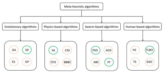
Figure 5.
Classification of metaheuristic optimization methods and the selection of used algorithms in this paper (in green circles): Genetic algorithm (GA), differential evolution (DE), evolution strategy (ES), genetic programing (GP), simulated annealing (SA), charged system search (CSS), central force optimization (CFO), big-bang big-crush (BBBC), particle swarm optimization (PSO), ant colony optimization (ACO), artificial bee colony (ABC), firefly (FF) algorithm, harmony search (HS), teaching learning-based optimization (TLBO), tabu search (TS), group search optimizer (GSO).
Optimization algorithms applied in this paper were selected in a way to examine at least one representative algorithm from each group of the metaheuristics. The simulated annealing (SA) algorithm was chosen from the physics-based algorithms. The vector-based differential evolution (DE) method as a representative of evolution-inspired algorithms was chosen, particularly due to its very good convergence [39]. The particle swarm optimization (PSO) and the firefly (FF) algorithm are the representatives of swarm-based algorithms since the PSO was proven to be very competitive with evolutionary and physically based algorithms [40] and the FF algorithm was already successfully applied in the CC optimization by the authors of the present paper [41].The last considered algorithm is the teaching-learning-based optimization (TLBO) from the category of the human-based algorithms and can be considered as the most recent algorithm among the algorithms applied in this paper.
The description of main ideas of these algorithms is provided in the following section and further information can be found in [40]. One of the crucial issues of meta-heuristics is a determination and proper tuning of their parameters. In the group of considered five meta-heuristics, the TLBO is an only parameter-less method, thus no parameter of the method needs to be determined. This can be beneficial in cases with rather simpler and fast optimization tasks, but the disadvantage is that the only option how to tune the algorithm is a proper selection of the random walk. Randomization is usually achieved with the use of pseudo-random numbers, based on some common stochastic processes, such as the Lévy flights or the Markov chain [40].
3.1. Simulated Annealing (SA)
The SA is one of the earliest and most popular metaheuristic algorithms developed in 1983 by Kirkpatrick et al. [42]. The SA is a trajectory-based, random-search technique for global optimization. It mimics the annealing process in materials processing when a metal cools and solidifies into a crystalline state with the minimum energy and growing crystals to reduce defects in the metallic structure. The annealing process involves a careful control of the temperature and its cooling rate, often referred to as the annealing schedule. The advantage of the SA against the deterministic methods is its ability to avoid being trapped in a local optimum solution. In this paper, the geometric cooling schedule and the temperature T during the annealing process is
with a stabilizing parameter and an initial temperature . In most practical applications, is frequently used [40]. If a new value of the objective function is worse than the previous one, the algorithm accepts the new solution only if the randomly generated number r from the uniform distribution [0, 1] satisfies the condition
where is the difference of the values of the objective function. This setting leads to faster stabilization and a more extensive local search.
3.2. Differential Evolution (DE)
The DE algorithm was initially developed in 1997 by Storn and Price [43]. The DE is a vector-based meta-heuristic algorithm, which has good convergence properties. This algorithm has some similarity to pattern search and genetic algorithms due to its use of crossover and mutation. The DE generates vectors of new parameters by adding the weighted difference between two population vectors to a third vector as
where is a mutation parameter referred to as the differential weight. The setup of is recommended as a good first choice [40]. Parameters of the mutated vector are then mixed with parameters of another predetermined vector to form the trial vector as
The parameter controlling the crossover probability is recommended to be [40], thus the j-th component has a 50% probability to be mutated, while the is a uniformly distributed random number. If the value of the objective function of the trial vector is better than the target vector, the trial vector replaces the target vector as
Each population vector serves once as the target vector. It is recommended that the population size should depend on the dimensionality of the problem [40].
3.3. Particle Swarm Optimization (PSO)
The PSO was developed by Kennedy and Eberhart in 1995 [44] and became one of the most widely used swarm-intelligence based algorithms due to its simplicity and flexibility. The behavior of the algorithm is based on the stochastically-drawn movement of particles in the space while they are attracted to the current best particle and to the current global best particle over the populations as
where α and β are learning and acceleration parameters, respectively, which are typically equal to 2 [40]; and and are random uniformly-distributed vectors having the values between 0 and 1. In each step, the particles are moved to new positions no matter if the new positions are better or not in terms of the value of the objective function as
Many improvements of the PSO have been published, including, for example, an accelerated PSO (APSO) [45] with an enhanced scheme allowing a better convergence rate.
3.4. Firefly (FF) Algorithm
Due to similarities between the PSO and the FF algorithm, the FF method received negative feedback within the research community. The inspiration between flashing patterns and the behavior of fireflies gave rise to the firefly algorithm proposed by Xin-She Yang [46] in 2010. A new position of a firefly in each generation is determined as
where the new position of the current firefly is determined by an attractiveness parameter and a randomization parameter . In this paper, the geometric annealing schedule is implemented, which reads
meaning that with the increasing number of generations, the randomness involved in the algorithm decreases. The attractiveness between fireflies is modeled as
where is the attractiveness at the distance , is the light absorption coefficient and is the Cartesian distance between the two fireflies i and j. The term for attractiveness is more significant for those fireflies that are closer to each other.
3.5. Teaching Learning-Based Optimization (TLBO)
The TLBO approach is one of the recently developed optimization algorithms [47]. This method exhibits great performance, which was assessed in [48]. The TLBO is a parameter-less algorithm, which consists of two phases. The first one is called the teacher phase, in which the group of learners (population) is normally distributed (with an obtained mean ) and learns from the teacher who is the learner with the best fitness among the whole population . In this phase, the learners attempt to get their values of the objective function towards the teacher’s value of the objective function as
where is a random number within the range [0, 1] and is the teaching factor defined as a heuristic step which can be either 1 or 2. The difference modifies the current vector and forms the new vector as
is accepted if it leads to better objective function, otherwise it remains unchanged and equals to vector of a previous generation . The second phase is called the learner phase, in which the learner shares knowledge and interacts with other different learners to further improve his/her performance. In this phase, the obtained new vector in teacher phase is set to , while is a randomly selected vector () from the learners and the new vector is
where is a random number within the range [0, 1]. Finally, the new vector is accepted if it provides a better value of the objective function value.
4. Results and Discussion
The computational model was set up with the geometry and configuration of the radial CCM operated in Třinec Iron and Steelworks in the Czech Republic. The CCM produces steel billets with the cross section of 150 mm × 150 mm, it has a tube-based water-cooled mold and the secondary cooling zone incorporates 178 water cooling nozzles. The length of the mold is 1000 mm and the radius of the radial part of the CCM is 8900 mm. The straightening of the curved strand starts at the distance of 14,255 mm from the meniscus (called the unbending point), where the strand is assumed to be fully solidified in order to withstand high tensile strain in this location. The secondary cooling zone is divided into six sections, each independently controlled and having a different set of cooling nozzles. The casting speed is set to 2.78 m/s and does not vary during the optimization. The target temperature distribution and cooling profile of secondary cooling zone was assumed as shown in Figure 6 (based on operational experience) and the optimization problem can be formulated as
where the objective function is the sum of average surface temperature errors in individual loops, d is the number of cooling loops, is the target average surface temperature in the i-th section of secondary cooling zone, is the calculated average surface temperature in the i-th section of the secondary cooling zone, is the maximum allowable surface temperature error set to 50 °C, is the metallurgical length, is the location of the unbending point of the CCM and is the average surface temperature at the unbending point. According to [11,12], the surface temperature at the unbending point must be higher than (which is considered 1100 °C in this work) and the average surface temperature in each secondary cooling zone must be higher than (which is considered 850 °C in this work) to avoid brittle regions with reduced ductility. Water flow rates through the cooling loops in the secondary cooling zone are also limited as specified in Table 1.
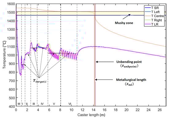
Figure 6.
Considered target temperature distribution along the CCM for the steel grade 18CrNiMo7-6, with the longitudinal temperature profiles depicted in the middle of strand faces T SR (small radius), T LR (large radius), T Left (left side), T Right (right side) and T Centre being the temperature in the core of strand.

Table 1.
Considered target water flow rates in the secondary cooling zone for given casting speed 2.78 m/s.
The aim of optimization was to determine casting conditions under which the sum of the average zone surface temperature errors is less than 50 °C. This accounts for about 8 °C of the temperature deviation per section in average, which is a rather hard condition to be achieved. In this work, the target water flow rates through the cooling loops in the secondary cooling zone were assumed as presented in Table 1 for the casting speed 2.78 m/s. In case of all optimization algorithms, the maximum number of algorithm-related operations was set to 1000. This means that the SA with a steady population was allowed to develop into 1000 generations. However, in swarm-based algorithms, such as the FF or the PSO, the population (including 10 individuals) was allowed to develop only into 100 generations. In this work, the population size was set identically to the number of generations applied in swarm-based algorithms (the FF and the PSO). In case of the DE, the number of individuals is recommended to be dependent on the dimensionality of a problem [40]. This recommendation was neglected, and the DE algorithm included the same number of individuals and maximum number of generations, such as were in FF and PSO. In the TLBO, the number of students was set to 10 individuals; however, due to the two-phase optimization approach (teacher and student phases), the maximum of 50 generations was established, whereas there were two evaluations of the solidification model for one individual in one generation. The recommended values of parameters for the SA, the DE and the PSO algorithms were defined in the previous chapter and the main parameters and their values applied in this work are listed in Table 2. The random walks involved in all algorithms were simulated in terms of the uniform distribution.
Table 2.
Used optimization parameters.
The 2.5D slice thermal-solidification numerical model, which was described in the foregoing section, was capable to simulate the temperature distribution of the cast strand in approximately 15 s on a PC with Intel(R) Core(TM) i7-3770 CPU @ 3.4GHz and 16 GB RAM. The size of the computational mesh 2.5 mm × 2.5 mm was set according to the mesh independency test mentioned above and with respect to appropriate treatment with boundary conditions, which were applied to all computational slices of thickness 25 mm. The majority (about 73%) of the computational time required by the numerical model is spent with a determination of boundary conditions, especially with the distribution of the heat transfer coefficients under cooling nozzles. As metaheuristics are random-based algorithms and a repeated execution of a particular algorithm under identical setup does not in general lead to the same result, the optimization study in this work included 500 runs with 100 runs per each algorithm. The maximum number of operations available to an algorithm per one run was considered 1000, as explained above, which gives the overall maximum of 500,000 evaluations of the heat transfer and solidification model. This approach was used to assess the stability of algorithms in terms of the optimal solution. The flow block diagram representing the introduced optimization process is shown in Figure 7.
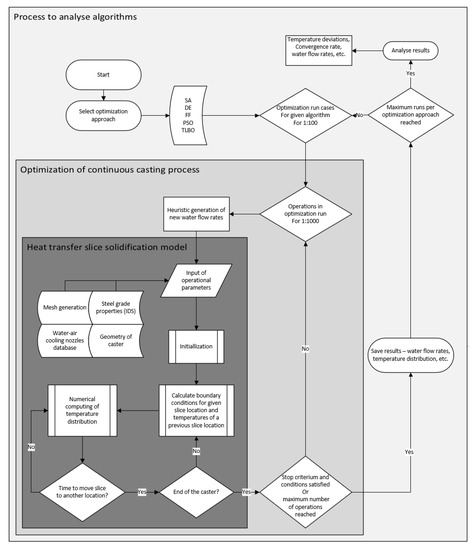
Figure 7.
Flow block diagram representing the applied optimization process.
According to Table 3 with the results, the overall best solutions were achieved with the use of the DE algorithm. In this case, the temperature error was 11.37 °C, with a slightly higher (by about 2.4 l/min) overall water flow rate through the secondary cooling zone when compared to the target solution. The only algorithm which achieved a solution with a lower overall water flow rate through the secondary cooling zone was the FF, as its best solution exhibits about a 2% lower water flow rate than the target solution. As for the temperature error of the FF for its best solution, it is about 21.4 °C, which is similar to those of the SA, the PSO and the TLBO. The highest mean-value water flow rate of about 756.6 l/min was achieved with the PSO algorithm. Figure 8 demonstrates the water flow rates for the best solution within the set of 100 runs. A fairly similar behavior in the first cooling loop for each metaheuristic algorithm can be seen, nevertheless the other cooling loops exhibit some minor deviations against the target water flow rates.
Table 3.
Mean-value temperature errors and water flow rates and the best temperature error and water flow rates (values in the brackets) for each algorithm for the casting speed of 2.78 m/s.
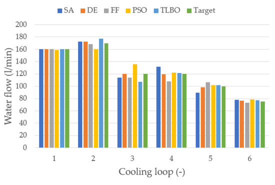
Figure 8.
The water flow rates through the secondary cooling zone of the best solutions of individual algorithms.
The overall results listed in Table 4 show that the only algorithm exhibiting a worse convergence rate than other algorithms is the PSO algorithm, with only 78 of 100 runs reaching the stop criterium. In case of the SA, the DE, the FF and the TLBO algorithms, the stop criterium was in the majority of runs reached. The FF algorithm reports even a 100% convergence success. The lowest mean-value and median-value number of operations performed by the algorithm to reach the solution was in case of the DE algorithm, which also exhibits the smallest variation of the number of generations needed to converge in each run, as depicted in Figure 9 where the median, the lower and upper quartiles for the number of operations are shown. The best (lowest) median value for the number of operations was achieved in case of the SA algorithm. On the other hand, the worst behavior in terms of the required number of operations was observed in case of the FF algorithm. This can be attributed to the geometric annealing schedule with an initial larger exploration and gradually increasing exploitation. The minimum number of operations needed to reach the solution was achieved for the SA, the DE and the PSO with 70, 68 and 73 operations per run, respectively. The convergence graph of individual algorithms, representing the averaged minimum temperature error (value of the objective function) reached by the algorithm in dependence to the number of operations, can be seen in Figure 10.
Table 4.
Overall results for the considered continuous casting (CC) optimization problem.
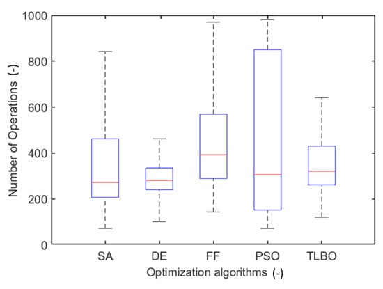
Figure 9.
Box plot with the number of operations needed to reach the solution: depicted in box plot with median, 25th percentile and 75th percentile.
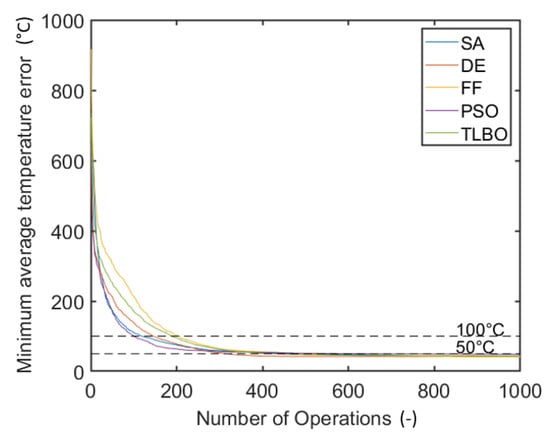
Figure 10.
The averaged minimum temperature error reached by the algorithm to particular operation.
If the stop criterium was set to a lower temperature error, the computational time increased. Based on the obtained results, it can be summarized that overall best behavior was exhibited by the DE algorithm. As for the computer implementation of the algorithms, none of the considered algorithms required more extensive experience but the SA algorithm can be considered as the easiest one from the implementation viewpoint. The worse behavior of the PSO algorithm could be due to inappropriately selected optimization parameters α and β, which lead to an entrapment in a local minimum, while the algorithm needs a lowest number of operations to reach the limit of the temperature error of 100 °C when compared to other algorithms, as demonstrated in Figure 10. The use of the enhanced PSO—the APSO—would improve the convergence rate of the PSO.
5. Conclusions
In the paper, five metaheuristic algorithms from each group of the metaheuristic classification were tested and assessed in the problem of continuous steel casting. A 2.5D slice thermal-solidification numerical model was developed and used for the optimization procedure. The objective of the optimization was to minimize the average temperature errors in each section of the secondary cooling zone within predefined temperature intervals by determination of appropriate water flow rates through cooling nozzles. The target values of the temperature intervals were specified in certain locations in the secondary cooling zone of the caster according to the literature review focusing on casting of high-quality final products.
- The best median value in terms of the number of operations needed by the algorithms to reach the solution was observed for the simulated annealing (SA) algorithm (with 271 operations per run and with the convergence rate of 96%) and for the differential evolution (DE) algorithm (with 280 operations per run and with the convergence rate of 99%).
- The best convergence rate was achieved in case of the FF algorithm in which all the runs reached the stop criterium, but with approximately 121 more operations per run than the DE algorithm.
- The particle swarm optimization (PSO) was surprisingly the worst algorithm among the considered algorithms, with 22 non-converged runs. A better behavior and performance of the algorithms could further be achieved by tuning of parameters of the individual algorithms.
- The teaching-learning-based optimization (TLBO), which is a method containing no algorithm-specific control parameters, exhibited medium performance among the considered algorithms and its convergence rate was 95%.
In conclusion, the DE algorithm was identified as the best performance algorithm for the considered control problem. Nevertheless, the performance of the SA, the FF and the TLBO algorithms was evaluated as good, which makes them also suitable for the solution of this kind of control problems.
Author Contributions
Conceptualization, M.B. and T.M.; Methodology, L.K.; Software, M.B.; Validation, M.B. and T.M.; Formal Analysis, M.B.; Investigation, M.B.; Resources, M.B. and T.M.; Data Curation, T.M.; Writing—Original Draft Preparation, M.B.; Writing—Review and Editing, M.B., T.M. and L.K.; Visualization, M.B.; Supervision, J.S.; Project Administration, J.S.; Funding Acquisition, J.S. All authors have read and agreed to the published version of the manuscript.
Funding
This work was supported by the Czech Science Foundation under contract No. 19-20802S “A coupled real-time thermo-mechanical solidification model of steel for crack prediction.” and by the research project funded by Brno University of Technology (FSI-S-20-6295).
Data Availability Statement
All necessary data are presented in the article. Other data and computer codes are not publicly available.
Acknowledgments
The authors acknowledge the financial support from Czech Science Foundation (project No. 19-20802S) and from Brno University of Technology (project No. FSI-S-20-6295).
Conflicts of Interest
The authors declare no conflict of interest. The funders had no role in the design of the study; in the collection, analyses, or interpretation of data; in the writing of the manuscript and in the decision to publish.
References
- Thomas, B.G. Review on Modeling and Simulation of Continuous Casting. Steel Res. Int. 2017, 89, 21. [Google Scholar] [CrossRef]
- Seetharaman, S. Treatise on Process Metallurgy; Elsevier: Oxford, UK, 2014; Volume 3, ISBN 9780080969886. [Google Scholar]
- Klimeš, L.; Štětina, J. A rapid GPU-based heat transfer and solidification model for dynamic computer simulations of continuous steel casting. J. Mater. Process. Technol. 2015, 226, 1–14. [Google Scholar] [CrossRef]
- Brimacombe, J.K. The challenge of quality in continuous casting processes. Metall. Mater. Trans. A 1999, 30, 1899–1912. [Google Scholar] [CrossRef]
- Santos, C.A.; Spim, J.A.; Garcia, A. Mathematical modeling of heat transfer in the Twin-Roll continuous casting process. Am. Soc. Mech. Eng. Heat Transf. Div. HTD 1998, 357, 133–138, ISBN: 8415683111. [Google Scholar]
- Brimacombe, J.K.; Sorimachi, K. Crack formation in the continuous casting of steel. Metall. Trans. B 1977, 8, 489–505. [Google Scholar] [CrossRef]
- Xia, G.; Schiefermüller, A. The influence of support rollers of continuous casting machines on heat transfer and on stress-strain of slabs in secondary cooling. Steel Res. Int. 2010, 81, 652–659. [Google Scholar] [CrossRef]
- Kulkarni, M.S.; Babu, A.S. Managing quality in continuous casting process using product quality model and simulated annealing. J. Mater. Process. Technol. 2005, 166, 294–306. [Google Scholar] [CrossRef]
- Cheung, N.; Santos, C.A.; Spim, J.A.; Garcia, A. Application of a heuristic search technique for the improvement of spray zones cooling conditions in continuously cast steel billets. Appl. Math. Model. 2006, 30, 104–115. [Google Scholar] [CrossRef]
- Kong, Y.; Chen, D.; Liu, Q.; Long, M. A prediction model for internal cracks during slab continuous casting. Metals (Basel) 2019, 9, 18. [Google Scholar] [CrossRef]
- Santos, C.A.; Spim, J.A.; Garcia, A. Mathematical modeling and optimization strategies (genetic algorithm and knowledge base) applied to the continuous casting of steel. Eng. Appl. Artif. Intell. 2003, 16, 511–527. [Google Scholar] [CrossRef]
- Cheung, N.; Garcia, A. Use of a heuristic search technique for the optimization of quality of steel billets produced by continuous casting. Eng. Appl. Artif. Intell. 2001, 14, 229–238. [Google Scholar] [CrossRef]
- Kim, K.; Yeo, T.J.; Oh, K.H.; Lee, D.N. Effect of Carbon and Sulfur in Continuously Cast Strand on Longitudinal Surface Cracks. ISIJ Int. 1996, 36, 284–289. [Google Scholar] [CrossRef]
- Böttger, B.; Apel, M.; Santillana, B.; Eskin, D.G. Relationship between solidification microstructure and hot cracking susceptibility for continuous casting of low-carbon and high-strength low-alloyed steels: A phase-field study. Metall. Mater. Trans. A Phys. Metall. Mater. Sci. 2013, 44, 3765–3777. [Google Scholar] [CrossRef]
- El-Bealy, M.O. On the Formation of Interdendritic Internal Cracks During Dendritic Solidification of Continuously Cast Steel Slabs. Metall. Mater. Trans. B 2012, 43, 1488–1516. [Google Scholar] [CrossRef]
- Suzuki, H.G.; Elyon, D. Hot ductility of titanium alloy: A challenge for continuous casting process. Mater. Sci. Eng. A 1998, 243, 126–133. [Google Scholar] [CrossRef]
- Fic, A.; Nowak, A.J.; Bialecki, R. Heat transfer analysis of the continuous casting process by the front tracking BEM. Eng. Anal. Bound. Elem. 2000, 24, 215–223. [Google Scholar] [CrossRef]
- Andersson, J.O.; Helander, T.; Höglund, L.; Shi, P.; Sundman, B. Thermo-Calc & DICTRA, computational tools for materials science. Calphad Comput. Coupling Phase Diagr. Thermochem. 2002, 26, 273–312. [Google Scholar] [CrossRef]
- Miettinen, J.; Louhenkilpi, S.; Kytönen, H.; Laine, J. IDS: Thermodynamic-kinetic-empirical tool for modelling of solidification, microstructure and material properties. Math. Comput. Simul. 2010, 80, 1536–1550. [Google Scholar] [CrossRef]
- Meng, Y.; Thomas, B.G. Heat-Transfer and Solidification Model of Continuous Slab Casting: CON1D. Metall. Mater. Trans. B 2003, 34B, 685–705. [Google Scholar] [CrossRef]
- Alizadeh, M.; Edris, H.; Shafyei, A. Mathematical Modeling of Heat Transfer for Steel Continuous Casting. Int. J. ISSI 2006, 3, 7–16, ISBN: 8415683111. [Google Scholar]
- Hardin, R.A.; Liu, K.A.I.; Kapoor, A.; Beckermann, C. A Transient Simulation and Dynamic Spray Cooling Control Model for Continuous Steel Casting. Metall. Mater. Trans. 2003, 34B, 297–307. [Google Scholar] [CrossRef]
- Tieu, A.K.; Kim, I.S. Simulation of the continuous casting process by a mathematical model. Int. J. Mech. Sci. 1997, 39, 185–192. [Google Scholar] [CrossRef]
- Tambunan, B. Simulation of Heat Transfer Solidification with Improved Latent Heat Parameter in Continuous Casting. In Proceedings of the Seminar National MIPA 2005; FMIPA: Depok, Indonesia, 25–26 November 2005; p. 7. [Google Scholar]
- Ji, Z.; Wang, B.; Xie, Z.; Lai, Z. Ant colony optimization based heat transfer coefficient identification for secondary cooling zone of continuous caster. IEEE Int. Conf. Integr. Technol. 2007, 558–562. [Google Scholar] [CrossRef]
- Zheng, P.; Guo, J.; Hao, X.J. Hybrid strategies for optimizing continuous casting process of steel. In Proceedings of the 2004 IEEE International Conference on Industrial Technology, Hammamet, Tunisia, 8–10 December 2004; Volume 3, pp. 1156–1161. [Google Scholar] [CrossRef]
- Rao, R.V.; Kalyankar, V.D.; Waghmare, G. Parameters optimization of selected casting processes using teaching-learning-based optimization algorithm. Appl. Math. Model. 2014, 38, 5592–5608. [Google Scholar] [CrossRef]
- Kulkarni, M.S.; Babu, A.S. Optimization of continuous casting using simulation. Mater. Manuf. Process. 2005, 20, 595–606. [Google Scholar] [CrossRef]
- Bhattacharya, A.K.; Debjani, S.; Roychowdhury, A.; Das, J. Optimization of continuous casting mould oscillation parameters in steel manufacturing process using genetic algorithms. In Proceedings of the IEEE Congress on Evolutionary Computation 2007, Singapore, 25–28 September 2007; pp. 3998–4004. [Google Scholar] [CrossRef]
- Jabri, K.; Dumur, D.; Godoy, D.; Mouchette, A.; Bèle, B. Particle swarm optimization based tuning of a modified smith predictor for mould level control in continuous casting. J. Process. Control. 2011, 21, 263–270. [Google Scholar] [CrossRef]
- Mauder, T.; Sandera, C.; Stetina, J. Optimal Control Algorithm for Continuous Casting Process by Using Fuzzy Logic. Steel Res. Int. 2015, 86, 785–798. [Google Scholar] [CrossRef]
- Incropera, F.P.; Bergman, T.L.; Lavine, A.S.; DeWitt, D.S. Fundamentals of Heat and Mass Transfer, 7th ed.; John Wiley & Sons: Hoboken, NJ, USA, 2011; ISBN 9780470501979. [Google Scholar]
- Zhang, J.; Chen, D.F.; Zhang, C.Q.; Wang, S.G.; Hwang, W.S.; Han, M.R. Effects of an even secondary cooling mode on the temperature and stress fields of round billet continuous casting steel. J. Mater. Process. Technol. 2015, 222, 315–326. [Google Scholar] [CrossRef]
- Raudenský, M.; Tseng, A.A.; Horský, J.; Komínek, J. Recent developments of water and mist spray cooling in continuous casting of steels. Metall. Res. Technol. 2016, 113. [Google Scholar] [CrossRef]
- Beyer, H.G.; Sendhoff, B. Robust optimization—A comprehensive survey. Comput. Methods Appl. Mech. Eng. 2007, 196, 3190–3218. [Google Scholar] [CrossRef]
- Blum, C.; Roli, A. Metaheuristics in Combinatorial Optimization: Overview and Conceptual Comparison. ACM Comput. Surv. 2003, 35, 268–308. [Google Scholar] [CrossRef]
- Mirjalili, S.; Lewis, A. The Whale Optimization Algorithm. Adv. Eng. Softw. 2016, 95, 51–67. [Google Scholar] [CrossRef]
- Maier, H.R.; Razavi, S.; Kapelan, Z.; Matott, L.S.; Kasprzyk, J.; Tolson, B.A. Introductory overview: Optimization using evolutionary algorithms and other metaheuristics. Environ. Model. Softw. 2019, 114, 195–213. [Google Scholar] [CrossRef]
- Das, S.; Suganthan, P.N. Differential evolution: A survey of the state-of-the-art. IEEE Trans. E Comput. 2011, 15, 4–31. [Google Scholar] [CrossRef]
- Yang, X.S. Nature-Inspired Optimization Algorithms; Elsevier Science Publishers, B.V.: Amsterdam, The Netherlands, 2014; ISBN 9780124167452. [Google Scholar]
- Mauder, T.; Sandera, C.; Stetina, J.; Seda, M. Optimization of the quality of continuously cast steel slabs using the firefly algorithm. Mater. Tehnol. 2011, 45, 347–350. [Google Scholar]
- Kirkpatrick, S.; Gelatt, C.D.; Vecchi, M.P. Optimization by simulated annealing. Science 1983, 220, 671–680. [Google Scholar] [CrossRef]
- Storn, R.; Price, K. Differential Evolution—A Simple and Efficient Heuristic for Global Optimization over Continuous Spaces. J. Global Optim. 1997, 11, 341–359. [Google Scholar] [CrossRef]
- Kennedy, J.; Eberhart, R. Particle swarm optimization. In Proceedings of the ICNN’95—International Conference on Neural Networks, Perth, WA, Australia, 27 November–1 December 1995; pp. 1942–1948. [Google Scholar] [CrossRef]
- Yang, X.S.; Deb, S.; Fong, S. Accelerated particle swarm optimization and support vector machine for business optimization and applications. Commun. Comput. Inf. Sci. 2011, 136, 53–66. [Google Scholar] [CrossRef]
- Yang, X.S. Firefly algorithm, stochastic test functions and design optimization. Int. J. Bio-Inspired Comput. 2010, 2, 78–84. [Google Scholar] [CrossRef]
- Rao, R.V.; Savsani, V.J.; Vakharia, D.P. Teaching-learning-based optimization: A novel method for constrained mechanical design optimization problems. CAD Comput. Aided Des. 2011, 43, 303–315. [Google Scholar] [CrossRef]
- Rao, R.V.; Patel, V. Multi-objective optimization of heat exchangers using a modified teaching-learning-based optimization algorithm. Appl. Math. Model. 2013, 37, 1147–1162. [Google Scholar] [CrossRef]
Publisher’s Note: MDPI stays neutral with regard to jurisdictional claims in published maps and institutional affiliations. |
© 2021 by the authors. Licensee MDPI, Basel, Switzerland. This article is an open access article distributed under the terms and conditions of the Creative Commons Attribution (CC BY) license (http://creativecommons.org/licenses/by/4.0/).