Statistical Soil Characterization of an Underground Corroded Pipeline Using In-Line Inspections

Abstract

Underground pipelines have a space-dependent condition that arises from various soil properties surrounding the pipeline (e.g., moisture content, pH, aeration) and the efficiency of protection measures. Corrosion is one of the main threats for pipelines and is commonly monitored with in-line inspections (ILI) every 2 to 6 years. Preliminary characterizations of the surrounding soil allow pipeline operators to propose adequate protective measures to prevent any loss of containment (LOC) of the fluid being transported. This characterization usually requires detailed soil measurements, which could be unavailable or very costly. This paper implements categorical measurements of soil properties and defect depth measurements obtained from ILI to characterize the soil in the surroundings of a pipeline. This approach implements an independence test, a multiple correspondence analysis, and a clustering method with K-modes. The approach was applied to a real case study, showing that more severe defects are likely located in poorly drained soils with high acidity.

1. Introduction

Corrosion is one of the main threats for onshore pipelines, either at the inner or outer walls. The external wall condition is subjected to a space-dependent degradation process favored by the varied soil conditions surrounding the pipeline, the pipe installation (e.g., underground, aboveground), and protection barriers (e.g., coatings, cathodic protection), among others. Considering the role of soil corrosiveness for underground pipelines, different authors have studied certain soil features to characterize more aggressive locations and take adequate protective measures. For instance, in this regard, soils with a higher concentration of chlorides, an acidic pH, and the presence of bacteria or fungi have been recognized to influence the external corrosion significantly [1].

Some studies have focused on power-law regression analysis from a degradation perspective, considering field or experimental measurements. Romanoff published a thorough analysis of underground pipelines based on 47 different soil types, with an exposure time greater than ten years and different soil aeration levels (i.e., good, fair, and poor) [2]. Similar power laws have been reported in the work of Kucera and Mattsson [3], Southwell et al. [4], and Velázquez et al. [5]. Kucera and Mattsson evaluated the general corrosion at atmospheric pressure. Southwell and co-workers fitted the data of pitting corrosion from 52 metal and alloys exposed to five different tropical environments for 16 years [4]. Finally, Velázquez et al. investigated the corrosion rates during three years in different soils in the south of Mexico, showing that corrosion aggressiveness could be shown to be in the following order: clay > loam > sand [5].

Other authors have considered the information recollected from in-line inspections (ILI) to characterize the surrounding soil. These inspections are commonly implemented every 2 to 6 years to monitor the entire condition of the pipeline. This approach uses a set of magnetic or ultrasonic sensors on a tool known as a pipeline inspection gauge (PIG) as a screening tool to support further maintenance or repair decisions. In this regard, Caleyo et al. [6] contemplated the statistical characteristics of the soil reported in [5] with consecutive ILI measurements to predict the probability distribution of the pit depth and pit growth rate. Wang and co-workers [7] developed a framework to cluster defects depending on their corrosion rates and they estimated a space-dependent corrosion rate probability density using soil measurements such as the resistivity or the soil pH. Other alternatives considered defect count data models such as Multivariate Negative Binomial [8] or Multivariate Poisson-Lognormal (MVPLN) models [9,10]. For instance, Wang and co-workers [10] implemented an MVPLN model to predict the pipe’s external corrosion. They used ILI data and both physical and chemical properties of the surrounding soil. All of these types of approaches require detailed soil measurements that may not be available for every underground pipeline, imposing some restrictions on the characterization of external pipe corrosion, especially when only qualitative information is available.

This paper presents an approach to characterize the soil in a pipeline’s surroundings and identify the main features of deep defects, considering ILI measurements and basic soil classification. This classification considers situations when continuous soil measurements are not available, and only general features can be used to describe the pipeline in segments. This means that the information from features such as soil drainage, depth, texture, and acidity are reported with categorical variables. This approach evaluates the relationship between the severity of corrosion and the soil features mainly with three methods: (i) an independence test using contingency tables and Chi-square tests; (ii) a multiple correspondence analysis (MCA) to identify possible relations among these soil features and the corrosion severity; and (iii) a clustering method with K-modes of the soil features favoring more severe corrosion.

The paper is structured as follows: Section 2 presents a brief description of the soil surrounding the pipeline. Section 3 reviews some of the main factors influencing external pipe corrosion. Section 4 describes the proposed methodology. Section 5 describes the case study of the surrounding soil and ILI measurements. Section 6 presents and discusses the main results of the proposed methodology. Finally, Section 7 presents some concluding remarks and some insights for further developments.

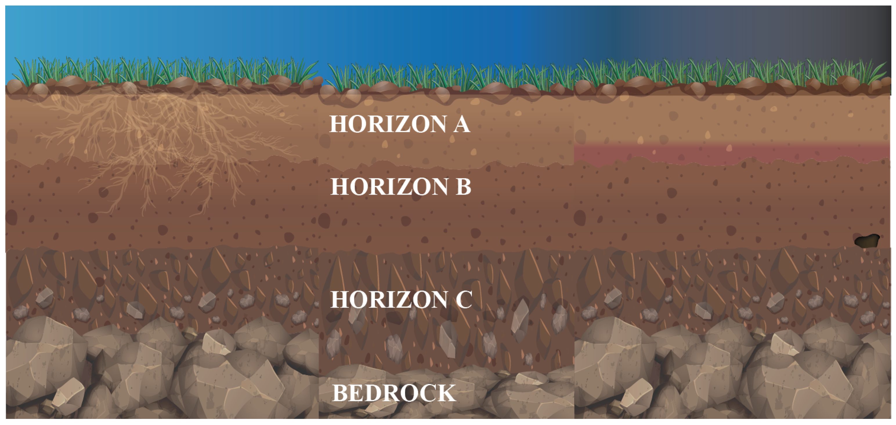
2. Brief Description of the Soil Surrounding the Pipeline

Soils are the consequence of historical climate conditions associated with rainfall and temperature, the relief or slope of the location, the surrounding organisms, minerals content, and biological/chemical activity [11]. Soils consist of a set of grains, such as mineral seeds and fragments of rock, with water and air in the grain vacuum (i.e., a three-state porous structure). Soils are subjected to chemical and mechanical processes such as disintegration (i.e., weathering) and erosion that define the soil’s evolution, which is affected mainly by water presence. For instance, water influences the transportation of nutrients and manages the moisture content from colloidal particles of clay and humus (i.e., organic matter by plant roots) [11]. The way the soil particles are rearranged may affect some local properties such as permeability (e.g., fine and coarse soils), strength due to fissures, stability from layers of different stiffness and strength by the presence of bonding influences [12].

Underground pipelines may lie on recent (entisols), developing (inceptsols) or mature geological deposits. The latter deposits exhibit a different mineral composition from the soil surface to the bedrock. In this regard, three horizons can be discriminated [13]:

• Horizon A (Eluvial zone): This zone is at the top of the soil profile; it directly contacts the atmosphere, receiving the rainfall and nutrients from the environment. In this zone, the biological activity is related to humus formation, and the leaching process of gravitational water produces more stable minerals (extracts of soluble minerals).
• Horizon B (Illuvial zone): This zone is rich in soluble minerals thanks to the leaching and weathering process in the overlying layer; however, this zone has low organic content.
• Horizon C: Weathering processes commonly leave this zone unaltered, and it tends to host little biological activity.

These zones are affected by two principal factors: temperature and rainfall [13]. An intensification of the rainfall may accelerate the leaching of soluble minerals at the top layer. An increase in temperature can accelerate the biodegradation of organic matter or chemical reactions during the weathering and leaching of soluble minerals. The depth of these horizons may change significantly, and their boundaries may not be defined clearly [11]. There is a different horizon, called the epipedon, formed near the surface, almost completely composed of destroyed rocks. This horizon is not the same as the eluvial zone (Horizon A); it may also include the illuvial zone if the soil that has been turned to black by organic matter covers the soil surface to the Horizon B [14]. An example of a soil profile is depicted in Figure 1.

These horizons depend on the surrounding climate conditions, producing particular soil profiles (see Figure 2). Following Jack and Wilmott’s work, a brief description of soils under arid, tropical, temperate and arctic conditions is presented [13]. A significant lack of rainfall water characterizes arid regions such as deserts. Thus, there is a minimal leaching process of soluble minerals for organic loading. Tropical climates are recognized to have significant amounts of rainfall water, which filters extensively soluble minerals. Besides, the warm temperature in tropical climates promotes the degradation and weathering of organic components in the eluvial zone. The result is a soil rich in iron and aluminum oxides (oxisols) that hides a facade of humic material that tends to be acidic. Temperate zones have a clear dependence on rainfall, and three types of soils can be recognized: mollisols, alfisols, and ultisols. Mollisols are under modest rainfall with a wide top layer that accumulates water. Alfisols are slightly wetter and represent more acidic soil. Ultisols are even wetter; they are subjected to warmer conditions, and they show a greater accumulation of clay at the Illuvial zone. Finally, under arctic conditions associated with a large tundra area, the freeze–defrost cycles produce mechanical weathering or a fragmentation of the parental rocks. Furthermore, the low temperature leads to an accumulation of wide organic layers. These soils are particularly complicated for buried pipelines because they can be displaced, thus producing a channel for groundwater flow.

3. Soil Factors Influencing External Corrosion

The soil structure and how the size particle is distributed, and these two factors combined, define soil physical parameters that affect the soil’s aggressiveness towards the external wall. The influences of the moisture content, resistivity, pH, soil aeration, and bacteria activity are summarized below.

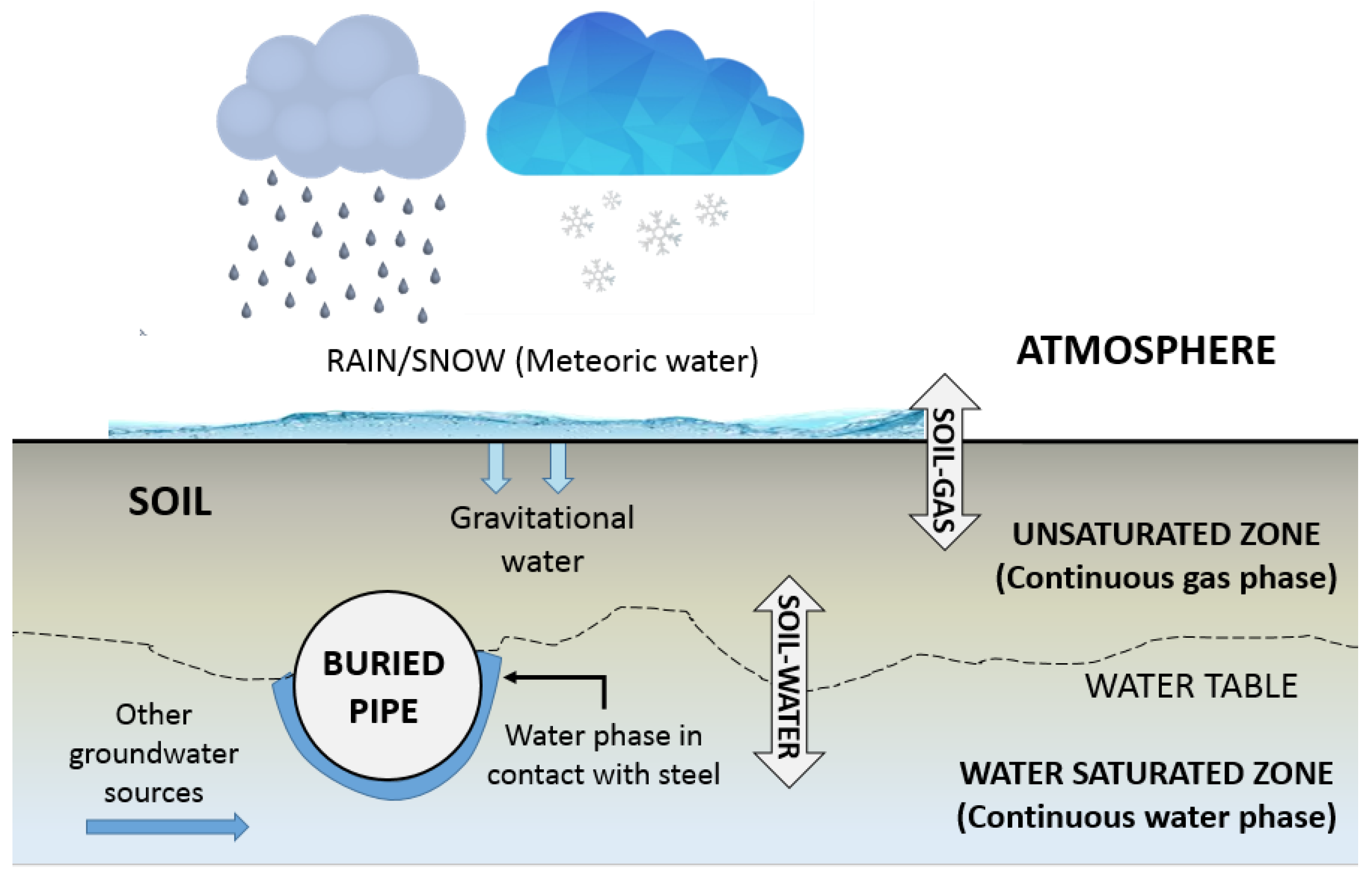
3.1. Moisture Content

Water in soils mainly has three sources, as illustrated in Figure 2; these are (i) meteoric water associated with rainfall or snowfall, (ii) water inside the soil void pores, and (iii) groundwater from the water table, which is a layer that is permanently saturated with water. The amount of water in the soil (moisture content) is one of the main factors contributing to the external corrosion of steel pipelines because it acts as an electrolyte for the corrosion process. Several authors have remarked that corrosion rates increase for wetter soils [15]; however, this content has been reported to reach a maximum for an intermediate saturation [16]. Some examples of this pattern include the work reported by Gupta and Gupta for mild steel specimens in sandy, sandy loam, and loamy soils, where loam is composed of sand (40%), silt (40%) and clay (20%). They found a limit of 65% of water capacity [17]. Noor and Al-Moubaraki evaluated the metal loss of X60 steel at different locations in Saudi Arabia, obtaining a maximum corrosion rate in soils with 10% of moisture content [18]. Schaschi and Marsh used sandy soils with sodium chloride solutions, obtaining minimum corrosion rates for almost dry (<5%) and saturated (>95%) conditions [19].

To explain the reaching of a maximum in the corrosion rate, consider that metal loss increases until the water saturates the soil pores, and the O₂ could not be supplied, which produces a reduction of the corrosion rates. Note that dry soil may have a high resistivity that reduces the corrosion rate. In contrast, an increment of moisture and temperature would produce a reduced soil resistivity, which, in turn, would support an exchange of the surrounding ions with the buried steel [20]. Although the moisture content depends on several factors such as the soil type, its role in soil corrosivity is highlighted. Moisture content has been used to identify aggressive soils; for instance, King remarked that soils with a moisture content greater than 20% would have an active metal surface favoring general corrosion [16]. These soils can be judged as having aggressive conditions. Otherwise, a corrosion attack would tend to follow localized pits [16]. As reported by Pereira et al., soil moisture less than 20% is associated with high soil resistivity, which decreases until reaching minimum resistivity by adding water [21].

3.2. Resistivity

Soil resistivity is defined as the soil’s capacity to resist electric current; a lower resistivity would imply saltier groundwater. Several authors have remarked that corrosion rates may increase with lower resistivity, as shown in

Table 1. Soil aggressiveness based on the resistivity and redox potential [13,26].

Aggressiveness	Resistivity (Ω ·cm)	Redox Potential mV
Mild-to-non corrosive	>5000	>400 *
Moderate corrosion	2000–5000	200–400
Corrosive	700–2000	100–200
Very corrosive	<700	<100

* >430 for clays. Ω denotes Ohm and V volts.

following the recommendations of King [16]. This table classifies the soil’s aggressiveness in terms of redox potential and resistivity. Authors such as Kulman [22] and Miller et al. [23] have reported alternative classes of soil resistivity [13,24,25]; however, in general, all researchers agreed that the soil tends to be more corrosive when the resistivity is reduced. Overall, smaller resistivity would accelerate macro-galvanic corrosion cells, triggering localized corrosion, and not micro-galvanic corrosion cells associated with uniform corrosion. However, Jack and Wilmott remarked that this dependency might be valid only in metals without cathodic protection, which are suggested to exhibit better performance [13].

Some physical parameters affecting the soil resistivity include the soil porosity, the soil compaction, the content of soluble ions, and the groundwater conductivity [13,16]. For instance, the resistivity would be reduced for soils with higher porosity or increased content of ions. King [16] developed a nomogram to correlate the soil resistivity, pH and corrosion rate; however, its prediction may be biased because it ignores the redox and microbial potentials.

3.3. Acidity of Soils, pH

Soil reactivity is measured based on the pH, with values ranging between 3.5 and 9.5. Acid soils (i.e., pH < 7) have saturated levels of ${\mathrm{H}}^{+}$ that usually arise from heavy rainfall and toxic leaching levels of manganese or aluminum, which can negatively affect the soil organisms [11]. Heavy rainfall produces exchanges of basic cations such as magnesium (${\mathrm{Mg}}^{+2}$) and calcium (${\mathrm{Ca}}^{+}$) from the colloids of the soil with the action of ${\mathrm{H}}^{+}$ from the water. In extreme rainfall areas, soil nutrients can even be washed out, leaving the soil without buffering capacity. On the contrary, low rainfall areas retain calcium ions, which may be in equilibrium with calcium carbonates [11]. Regarding the corrosion rates, several authors have reported that corrosion is favored by very acidic soils, while a passive state—i.e., one less affected by a corrosion environment—correspond with alkaline soils [20].

The soil reactivity is not a standalone indicator for soil corrosion and buried pipelines, as remarked by Wasim et al. [24] and King [16]. Some researchers such as Penhale, Rajani and Makar and Doyle have shown a weak or inexistent correlation between the corrosion rate and the soil pH [24]. King recognized that only measuring the pH without taking into account soil resistivity would provide ambiguous corrosion predictions. Depending on the resistivity, both very alkaline and acidic soils may have a relevant corrosion aggressiveness [16]. This result was confirmed by the review of Arriba-Rodriguez et al. [27], considering both the soil pH and the soil resistivity as reported by the BS EN 12501-2:2003 (Figure 3). Note that a medium–high corrosive category can be obtained even for very alkaline soils. However, King remarked that the soil acidity might influence the growth of sulfate-reducing bacteria (SRB) in alkaline soils, but it may support the growth of organisms that oxidize with iron ions looking for energy.

3.4. Aeration

Besides the soil moisture, the amount of oxygen trapped in the soil plays an essential role in the corrosion of buried steels. Cathodic and anodic reactions over the metal surface mainly depend on the water and oxygen in the soil. Overall, soils that are more saturated with water—i.e., with higher moisture and dissolved oxygen—would behave as a cathode. In contrast, soils with lower levels of moisture and dissolved oxygen would lie in an anodic area that favors the formation of pits [28]. The dissolved oxygen depends on different factors, including the soil density, the soil drainage, and compaction, and the soil depth. For instance, the dissolved oxygen increases for higher moisture until it reaches a critical point. Besides, the dissolved oxygen is reduced for a more profound soil [16].

According to Petersen and Melchers, buried pipelines would be subjected to three typical scenarios in which aeration may affect the integrity of the pipeline surface; they are summarized as follows [28]:

• Consider a change of aeration between the top and bottom of the pipeline, which could be obtained by installing a pipeline in undisturbed soil and a permeable backfill such as sand.
• Contemplate a difference in aeration because the water table is close to the bottom of the pipeline, where again the bottom of the pipeline would represent an anodic area that favors pits’ appearance.
• The final scenario corresponds to mixed of soils with different permeabilities; for instance, pipelines with a significant portion of clay adhered to metal or coating in a pipeline surrounded mostly by sand. This case would induce an anodic area in the section in contact with the less permeable soil [28].

3.5. Bacteria Activity

The activity of bacteria is a significant issue for pipelines, known as microbiologically influenced corrosion (MIC). Overall, the bacteria can be attached to the metal surface, producing biofilms that would degrade the surface by a series of biochemical reactions associated with bacterial growth and reproduction [29]. One of the most common types of bacteria found in soils is sulphate-reducing bacteria (SRB), which are considered anaerobic bacteria located in soils, containing sulfate ions with low dissolved oxygen with a pH between 6 to 8 [24]. In well-aerated soils, the bacterial effect on the corrosion rate is not relevant. These bacteria use sulfates and nutrients, including organic acids and the results of the natural decomposition of organic matter from the surrounding soil, to produce ${\mathrm{H}}_2\mathrm{S}$ as a secondary product, which may later interact with the metal to form $\mathrm{FeS}$ [28]. Other types of bacteria found in soils include metal-reducing bacteria, slime-producing bacteria and acid-producing bacteria [24].

3.6. Main Links between Factors

Several parameters may affect the soil’s aggressiveness and they may interact with a buried structure such as a pipeline. Additional parameters were not considered in this review, such as cathodic and anodic exchange capacities, the soil temperature or the exposure time (for further details, please refer to [16,24,25,27]). The main factors influencing external corrosion include the type of soil that establishes a degree of aeration (level of dissolved oxygen), which, jointly with the soil moisture, affects the current resistivity directly and so the corrosion rate. Additional parameters include the total acidity shown in the soil pH, how the ionic species may interact, and the possibility of the action of sulfate or metal-reducing bacteria [27].

4. Correspondence between Corrosion Depth and Soil Properties: Proposed Methodology

The full-scale assessment began with an exploratory analysis of the correspondence between the depth of defects and the surrounding soil. This assessment contemplated only the soil’s general descriptors based on a Geographic Information System (GIS) in the absence of detailed measurements. Suppose that we had J categoric soil features (e.g., soil acidity or permeability); the main objective was to describe the relationship between the features and the corrosion depth, which could be treated as a continuous quantitative variable or divided into categories to address non-linear behaviors [30]. For this work, the latter approach was considered based on the categories reported in

Table 2. Corrosion severity labels.

Category	Corrosion Depth (%t)
Low	0–24
Moderate	25–49
High	50–74
Very High	75–100

. These categories are only descriptive and do not consider the influence of the corrosion length, width, or the corresponding burst pressure. These categories were selected based on the recognized leak state limit of 85%t, where t is the pipeline thickness. Further criteria using the failure probability could also be implemented.

The correspondence between the corrosion categories and the J soil features were evaluated following three stages (Figure 4). The first stage evaluated each feature individually to inspect if it tended to be independent of the corrosion category using contingency tables and the ${\chi }^2$ test. The second stage implemented a multiple correspondence analysis (MCA) from the entire dataset to identify links among soil categories and correlations with the corrosion depth. The third stage considered a K-mode approach that clustered the combination of features with more profound corrosion defects, aiming to identify possible aggressive features of the soil. The procedure from the three stages is described in more detail below.

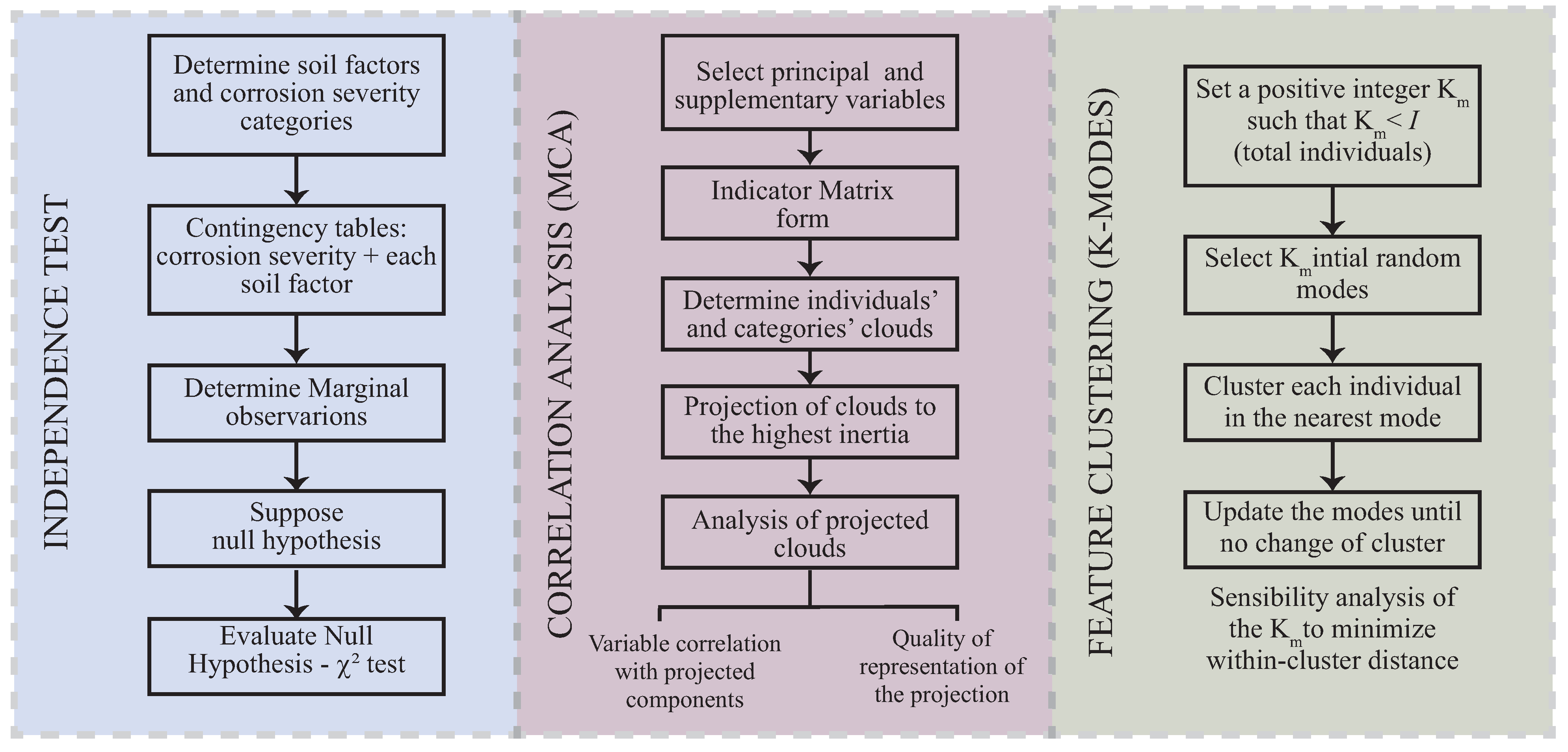
4.1. Soil Features and Corrosion Depth Independence

Consider one of the soil features described in Section 3, such as pH, resistivity, moisture or texture, and suppose that this feature has C mutually exclusive categories. The goal of the first analysis was to determine whether these categories depend on the severity categories reported in Table 2. For this purpose, the ILI records were summarized in contingency tables, and ${\chi }^2$ tests were implemented to evaluate a null hypothesis of independence between the two variables.

A contingency table uses the frequency of records in the row and column variables for each of their categories (i.e., R and C) that occur at the same time. In this case, $2\le R\le 4$, because high and very corrosion may not be observed. This table can be seen as a matrix $\left[n_{ij}\right]$ with a dimension of $R\times C$ whose components $n_{ij}$ are the number of records with the ith category in the row variable and the jth category in the column variable. Following this notation, the marginal observations (column/row sums) can be defined as $n_{i•}={\sum }_j^C{n}_{ij}$ for $i=1,\cdots ,R$ and $n_{•j}={\sum }_i^R{n}_{ij}$ for $j=1,\cdots ,C$, and the total number of observations is given by $n_{••}={\sum }_i^R{\sum }_j^C{n}_{ij}=N$ [31].

The objective of this approach was to evaluate the null hypothesis of independence between the two variables, which, in the context of this work, meant that the proportion of feature categories did not tend to be associated with a specific corrosion severity. We denote the probability of observing the ith row category and the jth column category as $p_{ij}$; under the null hypothesis, it follows that $p_{ij}=p_{i•}{p}_{•j}$, where $p_{i•}$ and $p_{•j}$ can be estimated as follows [31]:

$${\widehat{p}}_{i•}={\displaystyle \frac{n_{i•}}{N}},{\widehat{p}}_{•j}={\displaystyle \frac{n_{•j}}{N}}$$

Based on the above, the expected number of records is estimated by $E_{ij}=N{p}_{i•}{p}_{•j}$. The null hypothesis would be rejected if the expected number of records differed strongly from that reported by the sample obtained by the ILI measurement; therefore, the ${\chi }^2$ test was determined based on the statistic recommended by Pearson:

$${\chi }^2=\sum _{i=1}^R\sum _{j=1}^C{\displaystyle \frac{n_{ij}-E_{ij}}{E_{ij}}}$$

(1)

This statistic can be approximated using a ${\chi }^2$ distribution with $(R-1)(C-1)$ degrees of freedom, assuming that the frequencies follow a multinomial distribution [31]. A low statistic indicates relevant evidence for accepting the null hypothesis.

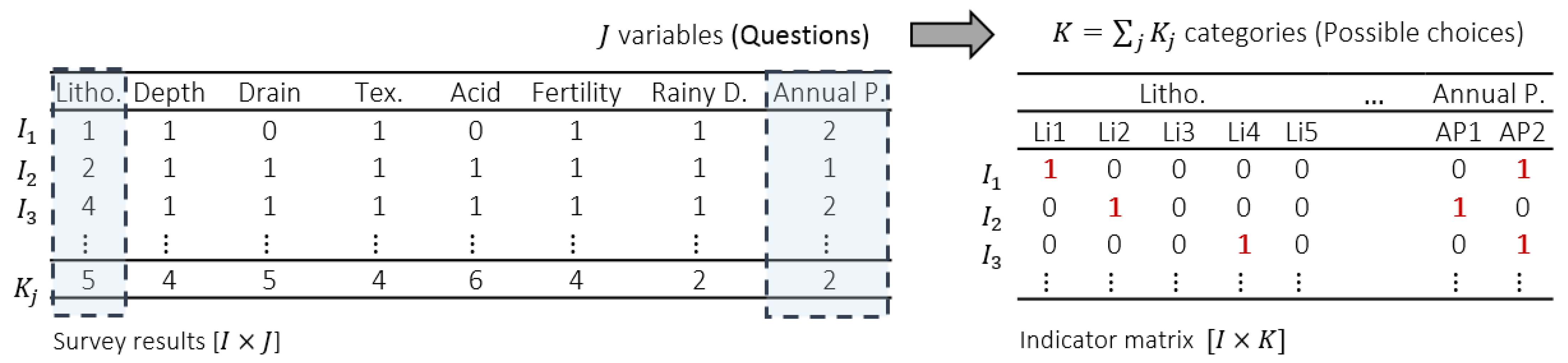
4.2. Multiple Correspondence Analysis of the Soil Features

Multiple correspondence analysis (MCA) is an exploratory analysis analogous to a principal component analysis (PCA) using categorical variables. Let I and J be the number of individuals and variables, respectively, as it would be in a survey with I responses of J multiple-choice questions. Each of the J “questions” has a specific number of possible answers denoted by $K_j$ that are known as categories; for instance, the corrosion variable has four categories, as depicted in Table 2. The objective of the MCA is to determine how similar the individuals (i.e., responses) are to identify possible relationships between variables (i.e., questions) and categories (i.e., possible answers). We denote as $x_{ij}$ the category selected by the ith individual of the jth variable and $X=\left[x_{ij}\right]$ as the $I\times J$ matrix dataset. This dataset can be expressed in a $I\times K$ indicator matrix, where $K={\sum }_j{K}_j$, as depicted in Figure 5. This figure shows the indicator matrix, in which instead of having the category selected by the individual ($x_{ij}$), an indicator vector of length $K_j$ is used for each variable with components $y_{ik}$, defined as follows [30]:

$$y_{ik}=\left\{\begin{array}{cc}1,\hfill & \mathrm{if}{x}_{ij}=k;\mathrm{the}{k}^{th}\mathrm{category}\mathrm{of}\mathrm{the}j\mathrm{th}\mathrm{variable}\hfill \\ 0,\hfill & \mathrm{Otherwise},\hfill \end{array}\right.$$

In this matrix, two types of variables are separated: active and supplementary. The active variables allow the determination of the leading associations and the supplementary variables as descriptors of the active ones; therefore, the corrosion variables were considered supplementary and the soil features as active variables for this work.

The individuals and the variables are in two clouds, denoted as $N_I$ and $N_K$, which have ${\mathbb{R}}^K$ and ${\mathbb{R}}^I$ dimensions, respectively. The dimensions of the clouds come from the rows and columns of the indicator matrix. The coordinates of the cloud of individuals are determined using proportional weights $p_k/J$ for each category k, where $p_k$ is the proportion of responses for the $k^{th}$ category and the weight of $1/I$ for each individual [32]. Both clouds evaluate the similarity among individuals and categories, depending on their closeness. For categorical variables, the differences of categories and the number of individuals in each category define the distances between individuals (and categories). These distances are defined in Equations (2) and (3).

$$\begin{array}{cc}\hfill & d_{i,i^{\prime }}^2={\displaystyle \frac{1}{J}}\sum _{k=1}^K{\displaystyle \frac{1}{p_k}}{(y_{ik}-y_{i^{\prime }k})}^2\hfill \end{array}$$

(2)

$$\begin{array}{cc}\hfill & d_{k,k^{\prime }}^2={\displaystyle \frac{p_k+p_{k^{\prime }}-2p_k{p}_{k^{\prime }}}{p_k{p}_{k^{\prime }}}}\hfill \end{array}$$

(3)

Based on the distance from a weighted individual in $N_I$ to the origin, it follows that if an individual has uncommon or particular categories—i.e., a small $p_k$ for some category k—then it is more separated from the origin. Similarly, rare categories would be more distant from the origin in the $N_K$ cloud. These clouds are correlated through transition relations, which can be described using the center of mass. The individuals correspond to a specific category or categories of certain individuals. These clouds are projected in a sequence of orthogonal axes, aiming to describe the cloud’s total inertia. This inertia is defined as follows [30]:

$$Inertia\left(N\right)={\displaystyle \frac{K}{J}}-1$$

(4)

where N represents both $N_I$ and $N_K$ clouds. The directions that maximize the representation of the inertia determine the components.

The results have two main numerical indicators; namely, the representation of the inertia in each component and the contribution or the quality of an individual/category. We denote as $\eta (v_j,F_s)$ the correlation of the jth variable and the s component, and the inertia represented in the s component (also reported as the eigenvalue) can be described as [32]

$${\lambda }_s={\displaystyle \frac{1}{J}}\sum _{j=1}^J{\eta }^2(v_j,F_s)$$

(5)

The amount of represented inertia is less than in PCA; in this case, it would be as high as $J/(K-J)$, so more components would be required to describe the entire inertia. However, Husson [32] recommends considering only those components with a percentage of inertia more significant than $1/J$, which corresponds to the average of non-zero eigenvalues. Husson et al. [30] remarked that ${\lambda }_s$ is also known as the eigenvalue because the MCA is essentially a correspondence analysis approach from the indicator matrix, where the projections come from a matrix diagonalization, and the eigenvalues are the extracted inertia. The projections occur in the direction of the eigenvectors.

This contribution describes the ratios of the inertia projected by an individual/category and the inertia projected from the entire cloud (in a given component). The quality of representation corresponds with the ratio of the inertia projected and the total inertia of the individual/category. This can also be described with the square cosine of the angle formed between the two inertias. It indicates the level of association between the categories and a given component [30]. In this work, the package of “FactoMineR” in R is implemented to evaluate the MCA results [33].

4.3. Soil Aggressiveness Clusters: K-Modes Approach

The previous analysis implements an MCA approach to detect a possible relationship between the J variables (soil features) and the corrosion categories. This section seeks to identify the combinations of variables reporting a more severe corrosion condition on the pipeline. For this purpose, the K-modes algorithm proposed by Huang [34] is implemented, which mostly follows the same principle of the unsupervised clustering of K-means with categorical data.

Instead of using a dissimilarity metric (e.g., Euclidean distance in K-means), the approach proposed by Huang uses a similar principle of the distance between individuals and categories to the one shown above for the MCA. Consider two individuals X and Y with m attributes (or categorical variables), Huang defined the total mismatches between them as follows [34]:

$$d(X,Y)=\sum _{j=1}^m\delta (x_j,y_j)$$

(6)

where $\delta (x_j,y_j)$ is a function that is equal to 1 only if $x_j\ne y_j$ and otherwise is equal to 0. Based on these mismatches, Huang defined the following dissimilarity measure:

$$d_{{\chi }^2}(X,Y)=\sum _{j=1}^m{\displaystyle \frac{(n_{x_j}+n_{y_j})}{n_{x_j}{n}_{y_j}}}\delta (x_j,y_j)$$

(7)

where $n_{x_j}$ and $n_{y_j}$ are the number of total individuals with categories $x_j$ and $y_j$ for the jth attribute (variable).

Let $Q=[q_1,\cdots ,q_m]$ be a vector in which each component $q_j$ corresponds to one of the $K_j$ possible categories for the jth attribute. The objective is to find Q such that it minimizes [34]

$$D(Q,X)=\sum _{i=1}^{n}d(X_i,Q)$$

(8)

where $X$ is the set of n individuals $X_i$, and the distance can be either the distance of total mismatches or the dissimilarity measure mentioned above. This distance is minimized based on a comparison of relative frequencies of the reported categories. The final K-modes algorithm starts by selecting $K_m$ initial modes; each individual is clustered in the nearest mode. The modes are updated after their relative frequencies are compared, and the procedure is repeated until there is no individual change of cluster. This work uses the classification and visualization package “klaR” in R to determine the desired modes and the classification of all individuals [35].

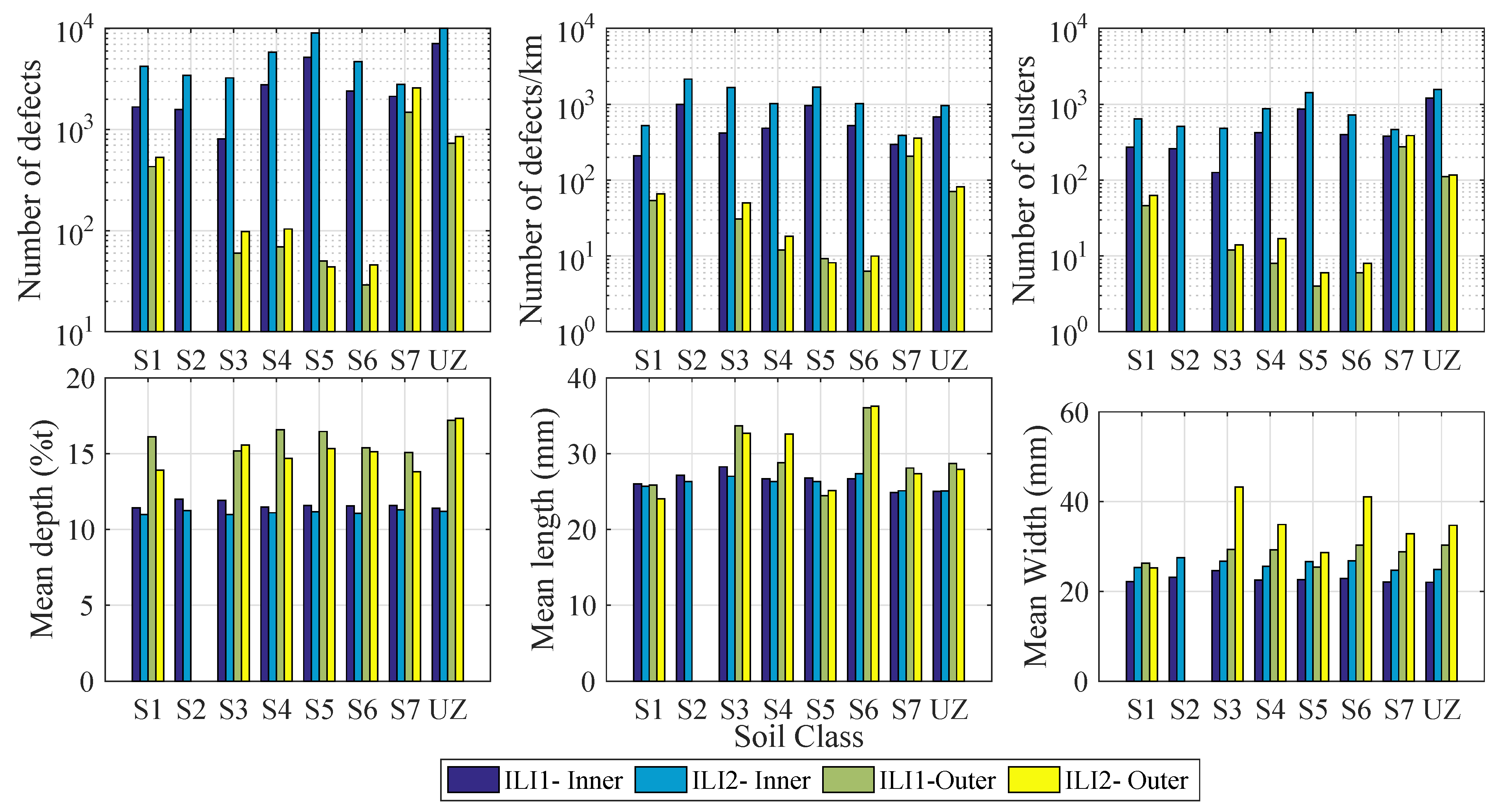
5. Case Study: Description and Spatial Dependencies

The case study used in this work is a 45 km long API 5LX52 pipeline; its height lies between 2560 and 2660 m above sea level, and it has six main valves. The pipeline has welded covers, supports and flanges along the route. The pipeline is mainly localized in a plain terrain with inclinations lower than 7°; it crosses two mountain sections and two urban zones. The climate is mainly cold–dry, but there are also cold–humid zones. The mean length for the pipe joints is 10.7 m, and the welded cover is 0.7 m. Near kilometer 33, there is a river crossing, whereas the last 10 km are close to urban zones (for further details, please refer to Amaya-Gómez et al. [36]).

The pipeline has a nominal wall thickness of 6.35 mm and an external diameter of 273.1 mm. The analysis presented here is based on data obtained from two consecutive ILI measurements two years apart. Both ILI inspections report small fluctuations in the mean operating velocity (around 2.2 m/s) and an operating temperature from 27 to 34 °C. More significant corrosion rates could be expected near the fifth and 15th kilometers, as these segments reported higher temperatures. According to the ILI report, the pipeline diameter is maintained along the entire abscissa; the wall thickness exhibits greater variability due to the location of welded covers, valves, dents and manufacturing flaws. The defect measuring tool was a magnetic flux leakage (MFL) sensor. Based on information reported in Amaya-Gómez et al. [37] about the inspection vendor, a circumferential uncertainty of 5° was assumed during the inspection. The measurement uncertainties of the defect depth, length and width are given by $d_{ILI}=d_{real}\pm {ϵ}_d$, $l_{ILI}=l_{real}\pm {ϵ}_l$, and $w_{ILI}=w_{real}\pm {ϵ}_w$, respectively, where $d_{ILI},l_{ILI}and{w}_{ILI}$ stand for the depth, length and width reported by the ILI tool, and ${ϵ}_d,{ϵ}_{l}and{ϵ}_w$ are the measurement errors. The measurement errors can be assumed to follow normal distributions centered at 0 with standard deviations obtained from the inspection vendors [38]. It is reasonable to assume that ${ϵ}_d=0.1t$ with t being the nominal wall thickness, ${ϵ}_l={ϵ}_w=11.70$ mm, considering a length and width accuracy of 15 mm with a confidence of 80% of the data. As a result of confidential agreements, further details of the case study cannot be provided.

Table 3. Pipeline segmentation based on the United States Department of Agriculture (USDA) soil classification.

Segment *	Category	Classification	ID
0.00–6.66 km	Complex	Pachic Melanudands (50%), Andic Dystrudepts (20%), Aeric Endoaquepts (15%), Aquic Hapludands (15%)	S1
6.66–8.2 km	Association	Humic Lithic Eutrudepts (35%), Typic Placudands (25%), Dystric Eutrudepts (25%)	S2
8.2–9.66 km	Complex	Pachic Melanudands (50%), Andic Dystrudepts (20%), Aeric Endoaquepts (15%), Aquic Hapludands (15%)	S1
9.66–11.61 km	Association	Humic Dystrudepts (60%), Typic Hapludalfs (40%)	S3
11.61–13.48 km	Complex	Pachic Haplustands (35%), Humic Haplustands (35%), Fluventic Dystrustepts (30%)	S4
13.48–14.86 km	Association	Aeric Epiaquents (60%), Fluvaquentic Endoaquepts (40%)	S5
14.86–15.89 km	Complex	Humic Dystrustepts (40%), Typic Haplustalfs (35%), Fluvaquentic Endoaquepts (25%)	S6
15.89–17.62 km	Association	Aeric Epiaquents (60%), Fluvaquentic Endoaquepts (40%)	S5
17.62–18.65 km	Complex	Humic Dystrustepts (40%), Typic Haplustalfs (35%), Fluvaquentic Endoaquepts (25%)	S6
18.65–18.84 km	Association	Typic Endoaquepts (40%), Aeric Endoaquepts (30%), Thaptic Hapludands (20%)	S7
18.84–21.40 km	Complex	Humic Dystrustepts (40%), Typic Haplustalfs (35%), Fluvaquentic Endoaquepts (25%)	S6
21.40–22.63 km	Association	Typic Endoaquepts (40%), Aeric Endoaquepts (30%), Thaptic Hapludands (20%)	S7
26.07–27.35 km	Complex	Pachic Haplustands (35%), Humic Haplustands (35%), Fluventic Dystrustepts (30%)	S4
27.35–28.22 km	Urban zone	-	UZ
28.22–30.52 km	Association	Aeric Epiaquents (60%), Fluvaquentic Endoaquepts (40%)	S5
30.52–33.10 km	Complex	Pachic Haplustands (35%), Humic Haplustands (35%), Fluventic Dystrustepts (30%)	S4
33.10–35.45 km	Association	Typic Endoaquepts (40%), Aeric Endoaquepts (30%), Thaptic Hapludands (20%)	S7
35.45–45.00 km	Urban zone	-	UZ

* Both in-line inspection (ILI) assessments did not include information of the segment from 22.63 to 26.07 km.

shows a broad classification of the soil along the pipeline, following the USDA’s taxonomy (United States Department of Agriculture). The pipeline has a bituminous coating of coal tar and an impressed current cathodic protection (ICCP) system. Coal tar is composed principally of aromatic hydrocarbons that constitute the foremost the liquid condensate of the distillation process from coal to coke [39]. Coal-tar-based coatings have exceptional moisture resistance; however, some disadvantages include poor light stability and possible cracks at the upper surface arising from an oxidation process due to a higher level of unsaturation [39]. Thicker layers can protect the pipeline, but a process of delamination is expected in a higher proportion than a polyethylene coat [40]. Unfortunately, further details of the ICCP were not provided by the pipe owner, nor by the company that performed the in-line inspection due to some confidential agreements.

The majority of defects were concentrated on the inner wall, which was expected due to the coal-tar coating; summary statistics of these data sets are depicted in

Table 4. Summary of corrosion defects along the abscissa.

Parameter	Mean (Coefficient of Variation)
	ILI-1 Inner Wall	ILI-2 Inner Wall	ILI-1 Outer Wall	ILI-2 Outer Wall
Average depth (%t)	5.49 (0.26)	5.29 (0.27)	7.28 (0.49)	6.77 (0.46)
Maximum depth (%t)	11.54 (0.21)	11.14 (0.19)	15.84 (0.46)	14.62 (0.43)
Length (mm)	26.07 (0.49)	26.07 (0.43)	28.07 (0.48)	27.37 (0.44)
Width (mm)	22.5 (0.40)	25.92 (0.53)	28.81 (0.67)	32.60 (0.75)
Number of defects	23,708	43,399	2862	4264

. Because further information about the shape of defects was not available in ILI, the maximum rather than the average depth for each defect is considered hereafter.

6. Results and Discussion

The case study crosses seven different soils and two urban zones (Table 3). Figure 6 summarizes the number of defects and clusters (DNV RP-F101 criterion), and the mean extent for each soil category. This figure shows that soil S2 has a higher number of defects per kilometer, followed by S3 and S5 for the inner wall. From these soils, S3 reported four times more defects in the second inspection, exhibiting the highest rate for both pipe walls. For the outer wall, there is a clear preference for soil S7, and in a lower proportion, for soils S1, and UZ. The number of defects from these three categories could be attributed to a higher proportion of clusters; however, the results indicate that almost 15% of defects for every soil type were sufficiently closed to interact with their neighbors. Regarding the defect extent, the mean depth, length, and width results do not suggest significant differences among the inner wall’s soil categories. On the contrary, the outer wall results indicate that defects in S3 and S6 tend to be longer and wider than the other soil types.

These soil classes are defined by particular features of their lithology, soil depth, drainage capacity, texture, acidity, fertility, and soil moisture (rainy days and precipitation). These features represented the “questions” in the survey analogy, where every defect acted as an individual answering the survey. We identified five categories of lithology, four for soil depth, five for drainage capacity, four for soil texture, five for acidity, four for fertility, two for rainy days per year, and two for annual precipitation.

Table 5. Categories of the soil features of the case study.

Soil Feature	Category	Description
Lithology	$L_{i1}$	Hydrogenic clastic deposits
	$L_{i2}$	Hydrogenic clastic deposits. Volcanic ashes in some sectors
	$L_{i3}$	Sandy clastic rock and clay silt
	$L_{i4}$	Sandy clastic rocks, carbonated clay silt with some deposits of volcanic ash
	$L_{i5}$	Volcaniclastic hydrogenic ash deposits
Depth *	$D_{e1}$	Deep to shallow (25 to 150 cm)
	$D_{e2}$	Deep to very deep (≥100 cm)
	$D_{e3}$	Moderate to deep (50 to 100 cm)
	$D_{e4}$	Very shallow (<25 cm)
Drainage	$D_{r1}$	Poor to moderately drained
	$D_{r2}$	Poor to very poor drained
	$D_{r3}$	Well to imperfectly drained
	$D_{r4}$	Well to moderately well drained
	$D_{r5}$	Well to poor drained
Texture **	$T_{x1}$	Fine texture
	$T_{x2}$	Fine to medium
	$T_{x3}$	Fine to moderately coarse
	$T_{x4}$	Medium to fine
Acidity	$A_{c1}$	Extremely to moderately acid (pH 3.5 to 6)
	$A_{c2}$	Extremely to strongly acid (pH 3.5 to 5.5)
	$A_{c3}$	Extremely acid to neutral (pH 3.5 to 7.3)
	$A_{c4}$	Moderately to slightly acid (pH 5.6 to 6.5)
	$A_{c5}$	Strongly to moderately acid (pH 5.1 to 6)
Fertility	$F_{e1}$	Low
	$F_{e2}$	Moderate
	$F_{e3}$	Moderate to high
	$F_{e4}$	Moderate to low
Rainy days per year	$R{D}_1$	100 to 150
	$R{D}_2$	100 to 200
Annual Precipitation	$A{P}_1$	1000 to 1500 mm
	$A{P}_2$	500 to 1000 mm

* Effective depth above gravel or bedrock. ** Fine texture includes clay, sandy clay, and silty clay. Medium texture includes silty clay loam and silt loam. Moderately coarse texture covers sandy loam, silty loam, loam, and silt.

describes the categories of each “question”. Note that the proposed categories are not entirely mutually exclusive because the information gathered included only ranges that may share values between the categories. For instance, the categories of total rainy days per year are 100–150 and 100–200 because they share ranges between 100 and 150 days. If detailed soil information were gathered for every kilometer or 200 m along the right-of-way (ROW) of the pipeline, as in Wang et al. [41], further insights would be obtained.

6.1. Correspondence Results with the Soil Categories

The initial stage evaluated the independence assumption between each soil feature and the corrosion severity labels low (0–24%), moderate (25–49%), high (50–74%), and very high (75–100%). For this purpose, contingency tables and a ${\chi }^2$-test were implemented, obtaining the results depicted in

Table 6. Chi-squared test results for the soil features categories.

Soil Feature	Parameter	ILI1-Inner	ILI1-Outer	ILI2-Inner	ILI2-Outer
Lithology	${\chi }^2$ test	15.56	23.34	5.52	33.36
	p-value	4.50$\times {10}^{-3}$	4.30$\times {10}^{-2}$	2.30$\times {10}^{-1}$	2.00$\times {10}^{-3}$
Depth	${\chi }^2$ test	1.30	26.80	4.41	23.89
	p-value	7.25$\times {10}^{-1}$	2.45$\times {10}^{-2}$	2.18$\times {10}^{-1}$	1.20$\times {10}^{-2}$
Drainage	${\chi }^2$ test	6.19	25.49	6.53	30.52
	p-value	1.65$\times {10}^{-1}$	5.85$\times {10}^{-2}$	1.63$\times {10}^{-1}$	6.50$\times {10}^{-3}$
Texture	${\chi }^2$ test	15.93	22.64	4.64	30.79
	p-value	3.00$\times {10}^{-3}$	3.10$\times {10}^{-2}$	2.05$\times {10}^{-1}$	3.00$\times {10}^{-3}$
Acidity	${\chi }^2$ test	17.57	9.92	2.02	19.44
	p-value	3.40$\times {10}^{-3}$	4.93$\times {10}^{-1}$	7.41$\times {10}^{-1}$	4.30$\times {10}^{-2}$ *
Fertility	${\chi }^2$ test	15.04	26.31	7.86	32.09
	p-value	3.50$\times {10}^{-3}$	2.45$\times {10}^{-2}$	4.65$\times {10}^{-2}$	1.00$\times {10}^{-3}$
Rainy days	${\chi }^2$ test	0.001	14.45	0.33	28.53
	p-value	1.00$\times {10}^0$	2.50$\times {10}^{-3}$	6.17$\times {10}^{-1}$	5.00$\times {10}^{-4}$
Annual precipitation	${\chi }^2$ test	0.25	19.39	3.40	19.65
	p-value	6.28$\times {10}^{-1}$	5.00$\times {10}^{-4}$	8.10$\times {10}^{-2}$	5.00$\times {10}^{-4}$

* If only low and moderate corrosion are considered, p-value > 0.05.

. This table presents the ${\chi }^2$ statistic in Equation (1) and the p-value under the null hypothesis of independence, considering 2000 Monte Carlo replicates for each soil feature and dataset. Based on a level of significance of 5%, the null hypothesis is rejected for the following features:

• ILI1-Inner: Lithology, texture, acidity, and fertility.
• ILI2-Inner: Fertility.
• ILI1-Outer: Lithology, soil depth, texture, fertility, rainy days, and annual precipitation.
• ILI2-Outer: Lithology, soil depth, drainage, texture, fertility, rainy days, and annual precipitation.

The obtained results suggest some interesting patterns. For the inner wall at the second inspection, the results indicate that the corrosion labels are almost independent of the soil features, as expected, except from a weak dependence with the fertility with a p-value of 0.0465. If a lower level of significance is contemplated (e.g., 1%), the null hypothesis of independence would not be accepted (actually, this result indicates that there is not sufficient evidence to reject the null hypothesis (fail rejection)). The outer wall results are entirely different; in this case, there is a perceived dependence with several soil features and the corrosion depth categories. Interestingly, the soil acidity was not included in this list when an additional comparison with only low and moderate labels are considered. For a level of significance of 1%, only the independence of rainy days and annual precipitation would be rejected for the first inspection. For the second inspection, all the features except the soil depth and the acidity would be rejected. The results mentioned above suggest that the corrosion severity levels are related in a higher proportion with the soil lithology, fertility, and texture, whereas the drainage and acidity seem to have weak dependences.

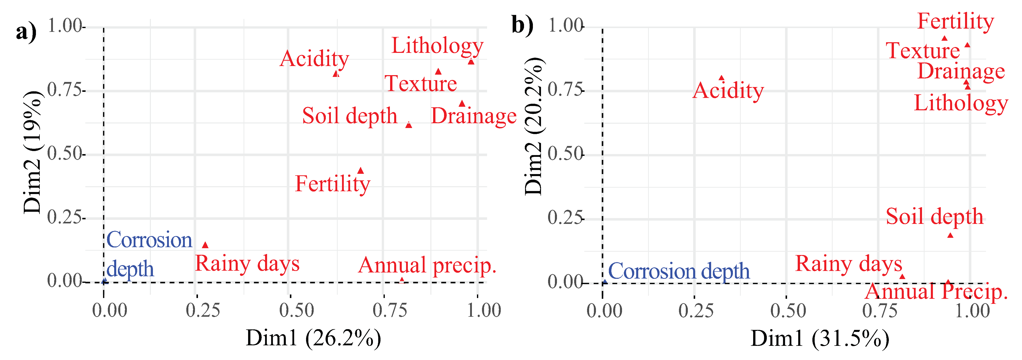
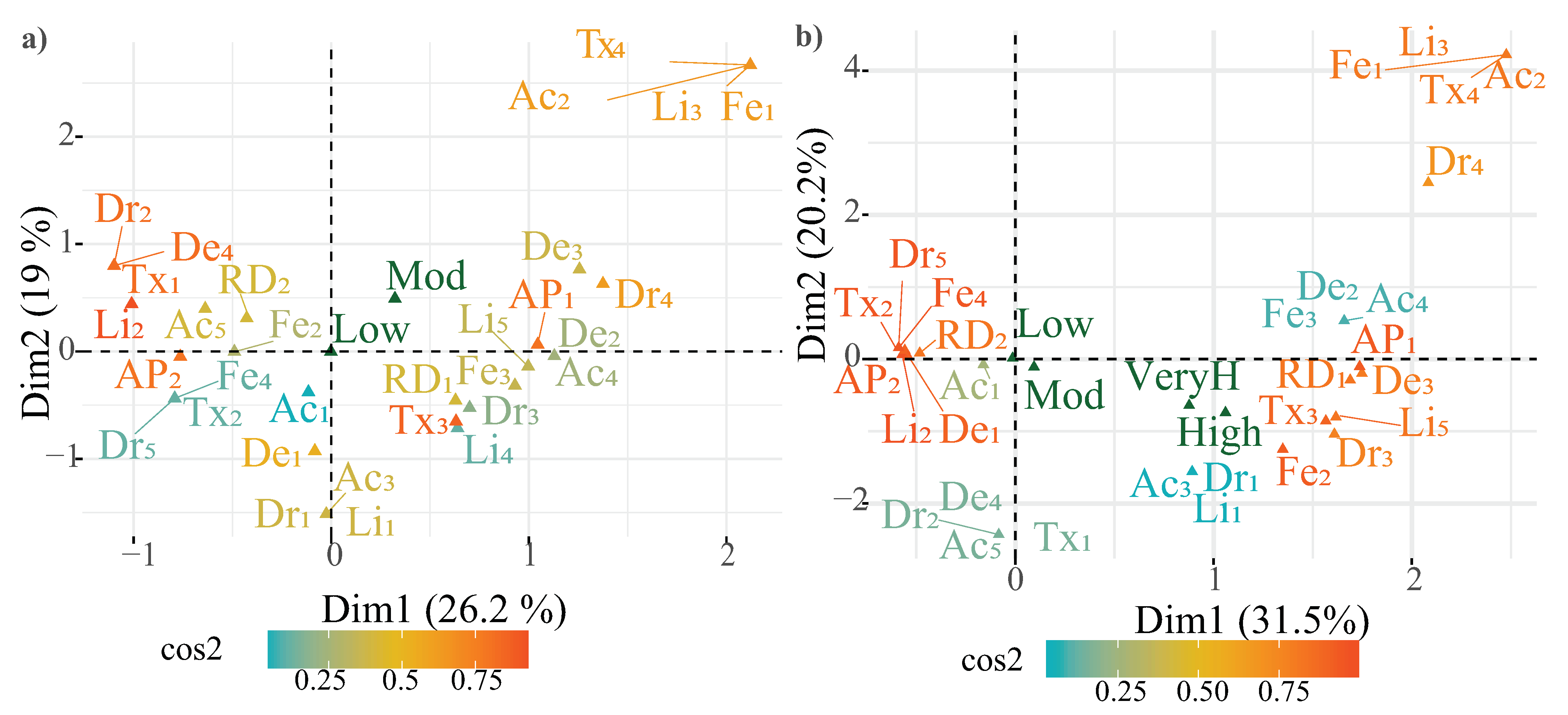
6.2. Multiple Correspondence Analysis (MCA) Results of the Soil Features Categories

We implemented all the soil features following a multiple correspondence analysis (MCA) in the next stage. The analysis considered the corrosion labels as a supplementary variable, which means that the corrosion categories did not contribute to constructing the orthogonal axes; they were used to describe soil features. In what follows, the results for the first inspection at both pipe walls is explained in more detail. The results are described based on the percentage of inertia explained by the components, the correlation of all the $v_j$ variables at each component $F_s$ (i.e., ${\eta }^2(v_j,F_s)$) and the factor (category) discrimination results based on the quality of the representation.

The inertia from the first two components covered 45.2% and 51.7% of the total variance of the ILI1-Inner and ILI1-Outer datasets, respectively. Thus, almost half of the individual and variable clouds’ variability could be explained by projecting the clouds to the plane formed by the first two components. The remaining inertia was distributed in lower proportions in four additional components at the inner wall and three for the outer dataset; however, only the first two components were evaluated. As an initial result, the correlation of the variables with the first two principal components for both pipe walls was compared, obtaining the results shown in Figure 7. In this figure, the corrosion depth is depicted in blue color because it is a supplementary variable, whereas the remaining variables were active, so they are represented with a red color. The axes of this figure correspond with the correlation ratios between each variable and each component. According to Husson, if this correlation ratio is close to unity for a given component, then individuals in the same category have similar coordinates for this component [30]. This figure is useful to describe some correlated variables in this projection depending on their proximity. Based on the results from both pipe walls, the annual precipitation and the rainy days were mainly correlated with the first component (i.e., the soil moisture). Furthermore, lithology, texture, drainage, and fertility were closely related in both cases, which may have produced redundant information. Regarding the inner wall (Figure 7a), the proximity between the variables of fertility and the total rainy days with the corrosion depth could indicate that they could have shown a higher proportion of corrosion severity. For the outer wall, Figure 7b shows that the soil depth and the soil acidity could also provide additional descriptions of the corrosion depth.

Regarding the MCA factor results, Figure 8 depicts the quality of the category representation obtained from both datasets. This figure shows a pattern known as the Guttman effect, where the distribution of factors looks like a parabola. According to Husson et al. [30], this effect indicates that some active variables (i.e., soil features) may be redundant, and the cloud of individuals may be constructed in a higher proportion for the first principal component. The authors also pointed out that this effect is favored for categorical variables following a given order, where one axis repels the smaller and most significant categories and another axis separates some extreme categories. As noted before, the lithology, texture and fertility are closely related primarily at the extreme value at the upper right, where a cluster formed by $L_{i3}$ (sandy clastic rock and clay silt), $T_{x4}$ (medium to fine), $F_{e1}$ (low fertility) and $A_{c2}$ (extremely to strongly acid) is recognized in both datasets, corresponding with the records reported in soil S3. Acidity categories $A_{c2}$ and $A_{c5}$ can be identified for the inner wall comparing the two extremes of the parabola, which are associated with a pH from 3.5–6 and 5.1–6, respectively. Similarly, for the outer wall, the extremes discriminated against the fertility categories $F_{e1}$ (low) and $F_{e4}$ (moderate to low), which would explain this pattern in both datasets.

We now consider the categories that better explained both planes. For the inner wall, Figure 8a indicates that the categories with a higher quality of representation (red color or $cos2>0.5$) are $L_{i2}$, $A{P}_2$, $A{P}_1$, $D_{e4}$, $D_{r2}$, $T_{x1}$, $T_{x3}$, $D_{e1}$, $D_{r4}$, $T_{x4}$, $A_{c2}$, $F_{e1}$ and $L_{i3}$. From these categories, the first dimension separates the annual precipitation and the soil depth. Higher annual precipitation is obtained at the right side (i.e., strong positive coordinate) with the $A{P}_1$ (1000–1500 mm) category compared with the lower annual precipitation of $A{P}_2$ (500–1000 mm) on the left side. Regarding the soil depth, note that on the left side (strong negative coordinate), the very shallow soils ($D_{e4}$) are found, while on the right side, deeper soils ($D_{e2}$, and $D_{e3}$) are found. The second dimension separates thinner and thicker soil textures. At the top (strong positive coordinate), the thinner categories $T_{x4}$ and $T_{x1}$ are found, as opposed to the moderately coarse texture of $T_{x3}$ with a strong negative coordinate. Regarding these descriptions, note that the low corrosion is at the center of mass of the cloud, and no preference is found based on the two dimensions. Moderate corrosion is more correlated with the positive coordinates of both dimensions—i.e., higher annual precipitation and thinner soil textures; however, there is no significant relation with a particular category. Recall that the corrosion depth is a supplementary variable, so the coordinates from both low and moderate categories are predicted using only the information provided by the performed MCA on the other active variables.

Regarding the results at the outer wall in Figure 8b, the categories with a higher quality of representation are $L_{i2}$, $A{P}_2$, $A{P}_1$, $D_{r5}$, $T_{x2}$, $F_{e4}$, $F_{e2}$, $T_{x3}$, $D_{e1}$, $L_{i5}$, $R{D}_2$, $R{D}_1$, $T_{x4}$, $A_{c2}$, $F_{e1}$, $L_{i3}$, $D_{e3}$ and $D_{r3}$. As in the inner wall, the first dimension separates higher annual precipitation ($A{P}_1$) on the right side with lower annual precipitations on the left side with $A{P}_2$. Furthermore, the right side concentrates a lower number of rainy days with the category $R{D}_1$ (100–150 days) with a high number of rainy days with $R{D}_2$ (100–200 days). The second dimension divides the well-drained soils with a positive strong coordinates with the categories $D_{r4}$ and $D_{r5}$ from those of poor drained soils with categories $D_{r3}$ and $D_{r2}$ with a negative coordinate. Regarding the corrosion categories, note that high and very high corrosion is preferred for poorly drained soils with a high annual precipitation. This result confirms the findings reported by different authors regarding soil moisture and aeration. Two groups can be also detected: the high and very high corrosion categories are related with $D_{e3}$ (moderate to deep), $F_{e2}$ (moderate) and $T_{x3}$ (fine to moderately coarse), whereas the low and moderate categories share distances with factors such as $D_{e1}$ (deep to shallow), $D_{r5}$ (well to poor drained), $T_{x2}$ (fine to medium) and $F_{e4}$ (moderate to low).

For the second inspection, similar results were obtained for the inner wall regarding how the two dimensions described the variable and individual cloud. For the outer wall, the Guttman effect was also found, but with a predominantly positive strong coordinate in the second dimension. In this case, the second dimension discriminates acid soils at the top and lower acid at the bottom, showing that high corrosion is preferred in locations with high annual precipitation.

The results indicated that deeper defects at the inner wall did not have any significant relationship with a particular category. Regarding the outer wall, the high and very high corrosion categories were preferred for poorly drained soils with high annual precipitation. This result matches one of the reported results of poorly drained soils; i.e., they trigger poor aeration and favor the corrosion process.

6.3. Corrosion and Soil Characteristics: Result of K-Mode Analysis

The last stage of the correspondence analysis between the corrosion categories and the soil features was the K-mode clustering, following the methodology reported by Huang [34]. As mentioned in Section 4.3, this algorithm requires an initial number of modes where the individuals will be clustered depending on their nearest neighbor. This procedure continues until there is no change in the way individuals are clustered. Therefore, sensitivity analyses with different modes were implemented to identify the number of modes, minimizing the within-cluster distance. Following an elbow (point of maximum curvature), we found that two modes were sufficient to handle this algorithm, except for low corrosion in the ILI2-Outer dataset, which required an additional mode.

Table 7. K-mode clusters per dataset and corrosion depth.

Dataset	Corrosion	Cluster	Points	Within Cluster	Litho.	Depth	Drain.	Tex.	Aci.	Fer.	R.Days	Precipi.
ILI1-Inner	Low	1	4512	16,142	$L_{i5}$	$D_{e1}$	$D_{r4}$	$T_{x3}$	$A_{c4}$	$F_{e3}$	$R{D}_1$	$A{P}_1$
		2	3489	4925	$L_{i4}$	$D_{e4}$	$D_{r2}$	$T_{x1}$	$A_{c5}$	$F_{e2}$	$R{D}_2$	$A{P}_2$
	Mod.	1	21	77	$L_{i3}$	$D_{e1}$	$D_{r4}$	$T_{x3}$	$A_{c2}$	$F_{e3}$	$R{D}_1$	$A{P}_1$
		2	16	15	$L_{i2}$	$D_{e4}$	$D_{r2}$	$T_{x1}$	$A_{c5}$	$F_{e2}$	$R{D}_2$	$A{P}_2$
ILI2-Inner	Low	1	9104	33,241	$L_{i5}$	$D_{e1}$	$D_{r4}$	$T_{x3}$	$A_{c4}$	$F_{e3}$	$R{D}_1$	$A{P}_1$
		2	5357	6570	$L_{i2}$	$D_{e4}$	$D_{r2}$	$T_{x1}$	$A_{c5}$	$F_{e2}$	$R{D}_2$	$A{P}_2$
	Mod.	1	43	148	$L_{i5}$	$D_{e1}$	$D_{r4}$	$T_{x3}$	$A_{c4}$	$F_{e3}$	$R{D}_1$	$A{P}_1$
		2	18	40	$L_{i2}$	$D_{e4}$	$D_{r2}$	$T_{x1}$	$A_{c5}$	$F_{e2}$	$R{D}_2$	$A{P}_2$
ILI1-Outer	Low	1	409	595	$L_{i5}$	$D_{e3}$	$D_{r3}$	$T_{x3}$	$A_{c1}$	$F_{e2}$	$R{D}_1$	$A{P}_1$
		2	1210	190	$L_{i2}$	$D_{e1}$	$D_{r5}$	$T_{x2}$	$A_{c1}$	$F_{e4}$	$R{D}_2$	$A{P}_2$
	Mod.	1	47	60	$L_{i5}$	$D_{e3}$	$D_{r3}$	$T_{x3}$	$A_{c1}$	$F_{e2}$	$R{D}_1$	$A{P}_1$
		2	90	25	$L_{i2}$	$D_{e1}$	$D_{r5}$	$T_{x2}$	$A_{c1}$	$F_{e4}$	$R{D}_2$	$A{P}_2$
	High *	1	2	1	$L_{i2}$	$D_{e1}$	$D_{r5}$	$T_{x2}$	$A_{c1}$	$F_{e4}$	$R{D}_2$	$A{P}_2$
		2	7	8	$L_{i5}$	$D_{e3}$	$D_{r3}$	$T_{x3}$	$A_{c1}$	$F_{e2}$	$R{D}_1$	$A{P}_1$
ILI2-Outer	Low	1	403	510	$L_{i5}$	$D_{e3}$	$D_{r3}$	$T_{x3}$	$A_{c1}$	$F_{e2}$	$R{D}_1$	$A{P}_1$
		2	75	0	$L_{i3}$	$D_{e3}$	$D_{r4}$	$T_{x4}$	$A_{c2}$	$F_{e1}$	$R{D}_1$	$A{P}_1$
		3	1861	185	$L_{i2}$	$D_{e1}$	$D_{r5}$	$T_{x2}$	$A_{c1}$	$F_{e4}$	$R{D}_2$	$A{P}_2$
	Mod.	1	121	20	$L_{i2}$	$D_{e1}$	$D_{r5}$	$T_{x2}$	$A_{c1}$	$F_{e4}$	$R{D}_2$	$A{P}_2$
		2	56	100	$L_{i5}$	$D_{e3}$	$D_{r3}$	$T_{x3}$	$A_{c1}$	$F_{e2}$	$R{D}_1$	$A{P}_1$
	High	1	7	15	$L_{i5}$	$D_{e3}$	$D_{r3}$	$T_{x3}$	$A_{c1}$	$F_{e2}$	$R{D}_1$	$A{P}_1$
		2	3	0	$L_{i2}$	$D_{e1}$	$D_{r5}$	$T_{x2}$	$A_{c1}$	$F_{e4}$	$R{D}_2$	$A{P}_2$

* This category includes both high and very high labels due to the low number of points of the latter.

presents the obtained results, including the number of points per cluster and the final within-cluster distance.

Regarding the clusters, Table 7 suggests some exciting results. Note that the acidity at the inner wall was mainly found to be $A_{c4}$ (moderately to slightly acid) and $A_{c5}$ (strongly to moderately acid), corresponding to a pH from 5.1 to 6. At the outer wall, acidity was almost entirely at $A_{c1}$ (extremely to moderately acid), which is associated with a pH between 3.5 and 6. Recall that acidity was considered to be independent of the corrosion severity labels once it was evaluated alone with contingency tables and the ${\chi }^2$ test. According to the corrosion literature, more acidic soil favors corrosion degradation, but it also depends on the associated resistivity (Table 3). This result confirms to a certain extent that corrosion degradation depends on several factors.

Other marked differences were in the categories of the soil depth, drainage, and texture, which affected the soil aeration, i.e., the amount of dissolved oxygen. The soil depth changed from $D_{e4}$ (very shallow) at the inner wall to $D_{e3}$ (moderate to deep) for the outer case—i.e., at additional soil horizons or a greater horizon depth, as described by Zabowski [42]—after a sample collection from 19 types of soil. Furthermore, both cases reported deep to shallow soil depths ($D_{e1}$) in a higher proportion. The clusters of the soil drainage at the inner wall focused on $D_{r2}$ (poorly to very poorly drained) and $D_{r4}$ (well to moderately well-drained) categories, which suggested that there was no relevant dependence between the drainage (and soil aeration) and the corrosion present at the inner wall, as expected. For the outer wall, the drainage was concentrated at the categories $D_{r3}$ (well to imperfectly drained) and $D_{r5}$ (well to poorly drained). Poorly drained soils usually trigger poor aeration and favor the corrosion process. This statement was supported in the case study; the corrosion points were clustered at $D_{r5}$ rather than $D_{r3}$. The number of moderate or high corrosion defects could also be favored with a drainage category of $D_{r5}$ considering how the pitting shape evolved. According to Romanoff [2], well-aerated soils tend to decrease the pitting rates due to an excessive amount of dissolved oxygen, favoring an oxidation process that forms a protective layer. Regarding the texture, the modes reported for the inner wall were located at $T_{x3}$ (fine to moderately coarse) and $T_{x1}$ (fine texture), whereas the modes were $T_{x3}$ and $T_{x2}$ (fine to medium texture) for the outer side, which again suggests that proper aeration was favored.

Regarding the results for the two inspections, note that the clusters from the outer wall were maintained (in a different order); those for the inner wall reported little changes regarding the lithology ($L_{i3}$ or $L_{i2}$ instead of $L_{i5}$) and acidity ($A_{c4}$ instead of $A_{c2}$). This result highlights how the clusters for the inner wall were indifferent to the soil corrosiveness when changing from extremely to strongly acid ($A_{c2}$) with a pH within 3.5–5.5 to a moderately to slightly acid soil ($A_{c4}$) with a pH from 5.6 to 6.5. The K-mode results allow us to describe some soil characteristics such as the acidity, texture, drainage, and soil depth in terms of those defects with moderate or high corrosion depth categories.

7. Conclusions

This paper sought to characterize the corrosiveness of soil surrounding an underground pipeline, considering a basic soil classification and depth measurements from in-line inspections. These measurements were classified based on categorical variables of low (0 to 25%t), moderate (25 to 50%t), and high (50 to 100%t) severities, which allowed us to identify the soil features more precisely. For this purpose, contingency tables and the ${\chi }^2$-test were implemented for each soil feature to assess the independence assumption with the corrosion severity labels. Besides, the proposed approach considered a correspondence analysis of the soil features and the depth of the corrosion defects using multiple correspondence analysis (MCA). Finally, this approach implemented a clustering method to describe the more profound (i.e., moderate and high) defects following a K-mode method, following a similar approach as K-means with continuous measurements.

Based on a real case study with two consecutive in-line inspections, the following results were obtained.

• The ${\chi }^2$-test results suggested that the fertility and texture categories are related in a higher proportion with the corrosion depth. Other related features include the soil depth, lithology, the number of rainy days, and the annual precipitation. Surprisingly, the results for acidity meant that we failed to reject the null hypothesis, although this is one of the main factors affecting the corrosion rate.
• The MCA results and the K-modes revealed that moderate to high corrosion depths are preferred for poorly drained soils with high annual precipitation and high acidity. This result confirms the reports by different authors about soil moisture and aeration. According to the corrosion literature, poorly drained soils usually trigger poor aeration and favor the corrosion process.
• Some categories that were more correlated included moderate to deep soil ($D_{e3}$), a fine-to-moderately coarse texture ($T_{x3}$) and moderate soil fertility ($F_{e2}$). The results of the K-modes method for the outer wall indicated that the acidity was almost entirely clustered in extremely to moderately acid (e.g., pH within 3.5 to 6), in moderate to deep soils and in well to poorly drained soils.

The proposed approach aims to help characterize the soil in an underground pipeline’s surroundings, considering the lack of continuous field measurements of parameters such as the resistivity or the pH. In this regard, information obtained from local or national Geographic Information Systems (GIS) can be integrated with valuable databases such as the one reported by the United States Department of Agriculture (USDA). In this regard, locations with high soil corrosiveness could be identified and validated with more detailed information. The advantage of the proposed approach lies in the analysis of soil categories that help us to understand the space-dependent degradation process to which the pipe’s external wall is subjected.

References

1. Castaneda, H.; Rosas, O. External Corrosion of Pipelines in Soil. In Oil and Gas Pipelines; John Wiley & Sons, Ltd.: Hoboken, NJ, USA, 2015; Chapter 20; pp. 265–274. [Google Scholar] [CrossRef]
2. Romanoff, M. Underground Corrosion; Technical Report; National Bureau of Standards Circular 579; United States Department of Commerce: Washington, DC, USA, 1957.
3. Kucera, V.; Mattsson, E. Chapter Atmospheric Corrosion. In Corrosion Mechanisms; Chemical Industries, Marcel Dekker: New York, NY, USA, 1987. [Google Scholar]
4. Southwell, C.; Bultman, J.; Alexander, A. Corrosion of Metal in Tropical Environments. Final Report of 16-Year Exposures; Technical Report; US Naval Research Laboratory: Washington, DC, USA, 1976. [Google Scholar]
5. Velázquez, J.; Caleyo, F.; Valor, A.; Hallen, J. Predictive Model for Pitting Corrosion in Buried Oil and Gas Pipelines. Corrosion 2009, 65, 332–342. [Google Scholar] [CrossRef]
6. Caleyo, F.; Velázquez, J.; Valor, A.; Hallen, J. Probability distribution of pitting corrosion depth and rate in underground pipelines: A Monte Carlo study. Corros. Sci. 2009, 51, 1925–1934. [Google Scholar] [CrossRef]
7. Wang, H.; Yajima, A.; Liang, R.Y.; Castaneda, H. Bayesian Modeling of External Corrosion in Underground Pipelines Based on the Integration of Markov Chain Monte Carlo Techniques and Clustered Inspection Data. Comput. Aided Civ. Infrastruct. Eng. 2015, 30, 300–316. [Google Scholar] [CrossRef]
8. Winkelmann, R. Seemingly Unrelated Negative Binomial Regression. Oxf. Bull. Econ. Stat. 2000, 62, 553–560. [Google Scholar] [CrossRef]
9. Chib, S.; Winkelmann, R. Markov Chain Monte Carlo Analysis of Correlated Count Data. J. Bus. Econ. Stat. 2001, 19, 428–435. [Google Scholar] [CrossRef] [Green Version]
10. Wang, X.; Wang, H.; Tang, F.; Castaneda, H.; Liang, R. Statistical analysis of spatial distribution of external corrosion defects in buried pipelines using a multivariate Poisson-lognormal model. Struct. Infrastruct. Eng. 2020, 1–16. [Google Scholar] [CrossRef]
11. Rhodes, C. Feeding and healing the world: Through regenerative agriculture and permaculture. Sci. Prog. 2012, 95, 345–446. [Google Scholar] [CrossRef] [PubMed]
12. Multiquip Inc. Soil Compaction Handbook; Technical Report; Multiquip Inc.: Carson, CA, USA, 2011. [Google Scholar]
13. Jack, T.R.; Wilmott, M.J. Corrosion by Soils. In Uhlig’s Corrosion Handbook; John Wiley & Sons, Ltd.: Hoboken, NJ, USA, 2011; Chapter 25; pp. 333–349. [Google Scholar] [CrossRef]
14. Soil Survey. Illustrated Guide to Soil Taxonomy; Technical Report; U.S. Department of Agriculture, Natural Resources Conservation Service: Lincoln, NE, USA, 2015.
15. Murray, J.; Moran, P. Influence of Moisture on Corrosion of Pipeline Steel in Soils Using In Situ Impedance Spectroscopy. Corrosion 1989, 45, 34–43. [Google Scholar] [CrossRef]
16. King, R. A Review of Soil Corrosiveness with Particular Reference to Reinforced Earth; Technical Report; Transport and Road Research Laboratory: Berkshire, UK, 1977; ISSN 0305-1315. [Google Scholar]
17. Gupta, S.; Gupta, B. The critical soil moisture content in the underground corrosion of mild steel. Corros. Sci. 1979, 19, 171–178. [Google Scholar] [CrossRef]
18. Noor, E.; Al-Moubaraki, A. Influence of Soil Moisture Content on the Corrosion Behavior of X60 Steel in Different Soils. Arab. J. Sci. Eng. 2014, 39, 5421–5435. [Google Scholar] [CrossRef]
19. Schaschl, E.; Marsh, G.A. Some New Views on Soil Corrosion. Mater. Prot. 1963, 2, 8–17. [Google Scholar]
20. Benmoussa, A.; Hadjel, M.; Traisnel, M. Corrosion behavior of API 5L X-60 pipeline steel exposed to near-neutral pH soil simulating solution. Mater. Corros. 2006, 57, 771–777. [Google Scholar] [CrossRef]
21. Pereira, R.; Oliveira, E.; Lima, M.; Brasil, S. Corrosion of Galvanized Steel Under Different Soil Moisture Contents. Mater. Res. 2015, 18, 563–568. [Google Scholar] [CrossRef] [Green Version]
22. Kulman, F. Microbiological Corrosion of Buried Steel Pipe. Corrosion 1953, 9, 11–18. [Google Scholar] [CrossRef]
23. Miller, F.; Foss, J.; Wolf, D. Soil Surveys: Their Synthesis, Confidence Limits, and Utilization for Corrosion Assessment of Soil. In Underground Corrosion; Escalante, E., Ed.; ASTM International: West Conshohocken, PA, USA, 1981; pp. 3–23. [Google Scholar] [CrossRef]
24. Wasim, M.; Shoaib, S.; Mubarak, N.; Inamuddin; Asiri, A. Factors influencing corrosion of metal pipes in soils. Environ. Chem. Lett. 2018, 16, 861–879. [Google Scholar] [CrossRef]
25. Cole, I.; Marney, D. The science of pipe corrosion: A review of the literature on the corrosion of ferrous metals in soils. Corros. Sci. 2012, 56, 5–16. [Google Scholar] [CrossRef]
26. Xanthakos, P. Ground Anchors and Anchored Structures; John Wiley & Sons: Washington, DC, USA, 1991. [Google Scholar]
27. Arriba-Rodriguez, L.; Villanueva-Balsera, J.; Ortega-Fernandez, F.; Rodriguez-Perez, F. Methods to Evaluate Corrosion in Buried Steel Structures: A Review. Metals 2018, 8, 334. [Google Scholar] [CrossRef] [Green Version]
28. Petersen, R.; Melchers, R. Long-Term Corrosion of Cast Iron Cement Lined Pipes. Corrosion & Prevention 2012: Corrosion Management for a Sustainable World: Transport, Energy, Mining, Life Extension and Modelling. 2012. Available online: http://hdl.handle.net/1959.13/1327302 (accessed on 15 November 2019).
29. Hamilton, W.A. Sulphate-reducing Bacteria and Anaerobic Corrosion. Annu. Rev. Microbiol. 1985, 39, 195–217. [Google Scholar] [CrossRef]
30. Husson, F.; Lê, S.; Pagès, J. Exploratory Multivariate Analysis by Example Using R; CRC Press: Boca Raton, FL, USA, 2011. [Google Scholar]
31. Everit, B. The Analysis of Contingency Tables; CRC Press: Boca Raton, FL, USA, 2019. [Google Scholar]
32. Husson, F. Multiple Correspondence Analysis, Agrocampus Ouest, Applied Mathematics Department. 2017. Available online: https://francoishusson.files.wordpress.com/2017/07/mca_course_slides.pdf (accessed on 15 January 2020).
33. Lê, S.; Josse, J.; Husson, F. FactoMineR: A Package for Multivariate Analysis. J. Stat. Softw. 2008, 25, 1–18. [Google Scholar] [CrossRef] [Green Version]
34. Huang, Z. A fast clustering algorithm to cluster very large categorical data sets in data mining. In Proceedings of the SIGMOD Workshop on Research Issues on Data Mining and Knowledge Discovery; Technical Report; University of British Columbia: Tucson, AZ, USA, 1997. [Google Scholar]
35. Weihs, C.; Ligges, U.; Luebke, K.; Raabe, N. klaR Analyzing German Business Cycles. In Data Analysis and Decision Support; Baier, D., Decker, R., Schmidt-Thieme, L., Eds.; Springer: Berlin/Heidelberg, Germany, 2005; pp. 335–343. [Google Scholar] [CrossRef]
36. Amaya-Gómez, R.; Bastidas-Arteaga, E.; Schoefs, F.; Muñoz, F.; Sánchez-Silva, M. A condition-based dynamic segmentation of large systems using a Changepoints algorithm: A corroding pipeline case. Struct. Saf. 2020, 84, 101912. [Google Scholar] [CrossRef]
37. Amaya-Gómez, R.; Sánchez-Silva, M.; Muñoz, F. Pattern recognition techniques implementation on data from In-Line Inspection (ILI). J. Loss Prev. Process Ind. 2016, 44, 735–747. [Google Scholar] [CrossRef]
38. Pandey, M.; Lu, D. Estimation of parameters of degradation growth rate distribution from noisy measurement data. Struct. Saf. 2013, 43, 60–69. [Google Scholar] [CrossRef]
39. Weldon, D. Failure Analysis of Paints and Coatings; John Wiley & Sons, Ltd.: Hoboken, NJ, USA, 2009; ISBN 978-0-470-69753-5. [Google Scholar]
40. Lee, S.; Oh, W.; Kim, J. Acceleration and quantitative evaluation of degradation for corrosion protective coatings on buried pipeline: Part II. Application to the evaluation of polyethylene and coal-tar enamel coatings. Prog. Org. Coatings 2013, 76, 784–789. [Google Scholar] [CrossRef]
41. Wang, H.; Yajima, A.; Liang, R.; Castaneda, H. A clustering approach for assessing external corrosion in a buried pipeline based on hidden Markov random field model. Struct. Saf. 2015, 56, 18–29. [Google Scholar] [CrossRef]
42. Zabowski, D.; Whitney, N.; Gurung, J.; Hatten, J. Total Soil Carbon in the Coarse Fraction and at Depth. For. Sci. 2011, 57, 11–18. [Google Scholar] [CrossRef]
Figure 1. Scheme of the soil profiles surrounding an underground pipeline.
Metals 11 00292 g001
Figure 2. Buried pipe exposure of the surrounding soil. Modified from Jack and Wilmott [13].
Metals 11 00292 g002
Figure 3. Soil corrosiveness based on the pH and resistivity according to BS EN 12501-2:2003
Metals 11 00292 g003
Figure 4. Scheme of the proposed methodology. MCA: multiple correspondence analysis.
Metals 11 00292 g004
Figure 5. Indicator matrix scheme.
Metals 11 00292 g005
Figure 6. General statistics based on the soil classes.
Metals 11 00292 g006
Figure 7. Variable correlation with the two principal MCA components ( η 2 ( v j , F 1 ) , η 2 ( v j , F 2 ) ) . (a) Inner and (b) Outer wall.
Metals 11 00292 g007
Figure 8. MCA factor results with a quality color description (quadratic cosine) for (a) ILI1-Inner and (b) ILI1-Outer. Labels are explained in Table 5.
Metals 11 00292 g008