Deep Learning Sequence Methods in Multiphysics Modeling of Steel Solidification

Abstract

The solidifying steel follows highly nonlinear thermo-mechanical behavior depending on the loading history, temperature, and metallurgical phase fraction calculations (liquid, ferrite, and austenite). Numerical modeling with a computationally challenging multiphysics approach is used on high-performance computing to generate sufficient training and testing data for subsequent deep learning. We have demonstrated how the innovative sequence deep learning methods can learn from multiphysics modeling data of a solidifying slice traveling in a continuous caster and correctly and instantly capture the complex history and temperature-dependent phenomenon in test data samples never seen by the deep learning networks.

1. Introduction

While developments of advanced steel solidification processes, such as metal-based additive manufacturing, are making steady progress, the field is still dominated by more traditional techniques, such as ingot, foundry, and continuous casting. Continuous casting produces over 95% of the world’s steel. Experiments are limited due to the molten steel’s harsh environment and the many process variables, which affect their complex multiphysics phenomena. Advancement of these established manufacturing processes mostly relies on the improved quantitative understanding gained from sophisticated multiphysics numerical models. Remarkable advances in computing technology and numerical algorithms in the last 30 years have enabled more realistic and accurate multiphysics modeling of steel solidification processes on high-performance computing systems.

Lee et al. [1], followed by Teskeredžić et al. [2], demonstrated multiphysics modeling of steel solidification by coupling a fluid flow of molten steel thermal-stress models of solidifying shell to predict solidification and stress formation on simplified casting geometries. Koric and Thomas [3] incorporated a bounded Newton-Raphson method from an in-house code [4] into Abaqus [5] commercial finite element code, which provided an order of magnitude performance increase in solving solidification thermo-mechanical problems, including the explicit finite element formulation [6]. Later Koric et al. [7] devised and validated a new enhanced latent heat method to convert spatial and temporal superheat flux data into the finite-element thermo-mechanical model of the solidifying shell and mold. The modeling approach was demonstrated via simulation of the multiphysics phenomena in continuous commercial casters of carbon steel grades [8], and lately, stainless steel grades [9]. Besides pure Lagrangian approaches, researchers have also lately used a combination of Eulerian approach in liquid, Lagrangian in solid, and Eulerian-Lagrangian in mushy (semi-solid) zones in treating multiphysics phenomena in steel solidification [10] as well as meshless numerical methods [11]. Application of steel solidification multiphysics models in crack formation mechanisms was also the subject of recent research works [12,13]. However, finding efficient and accurate multiphysics computational approaches, which can be widely applied on commodity computers, remains a challenge.

Lately, machine learning techniques, particularly deep learning, which is inspired by the biological structure and functioning of a brain, have accomplished significant successes in wide areas of science and engineering, such as natural language processing, computer vision, voice recognition, autonomous vehicle driving, medical diagnosis, and financial service. Numerical modeling in mechanics and material science is not an exception. Various surrogate deep learning data-driven models have been trained to learn and quickly inference the thermal conductivity and advanced manufacturing of composites [14,15], topologically optimized materials and structures [16,17], the fatigue of materials [18], nonlinear material response such as in plasticity and viscoplasticity [19,20], and many other applications.

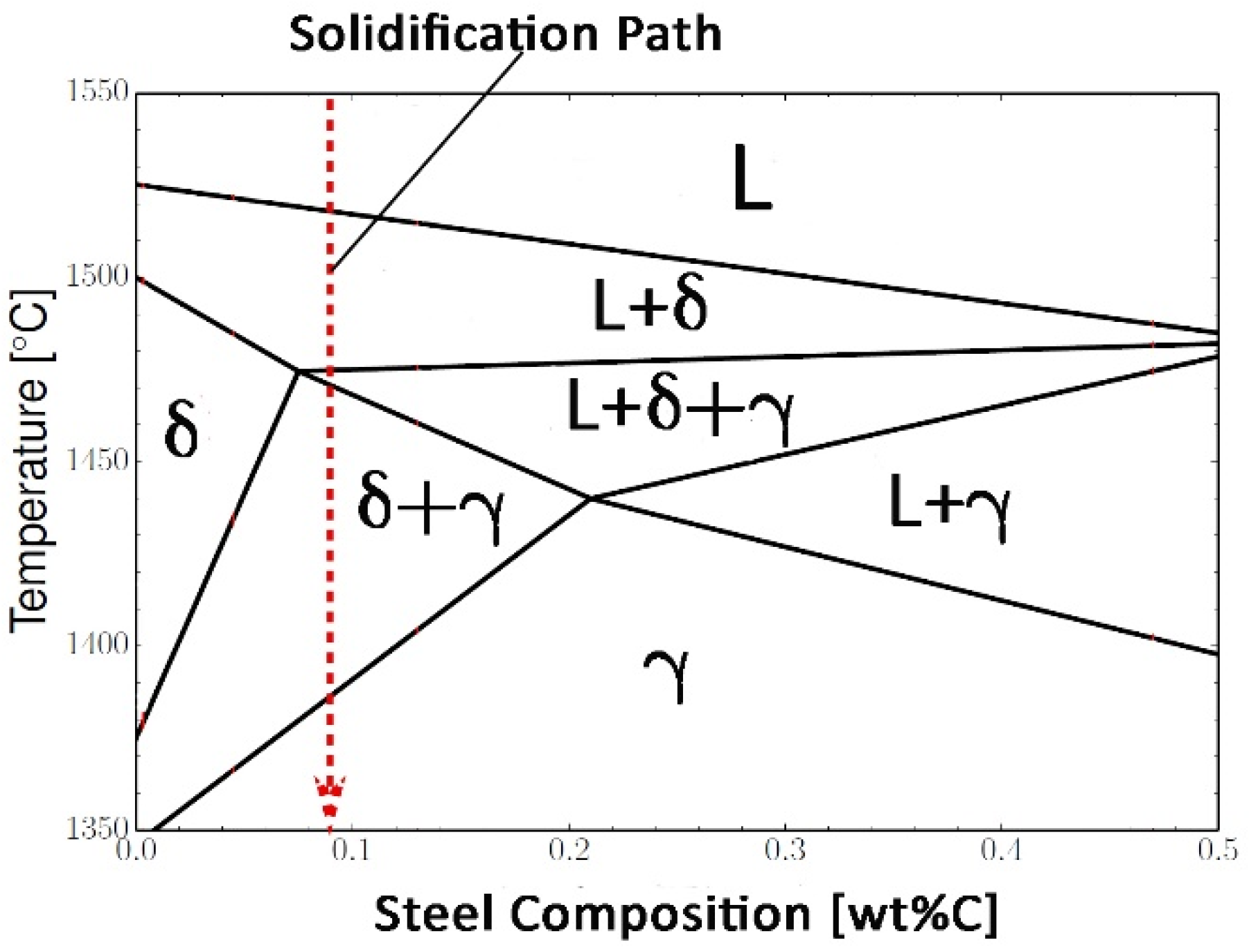
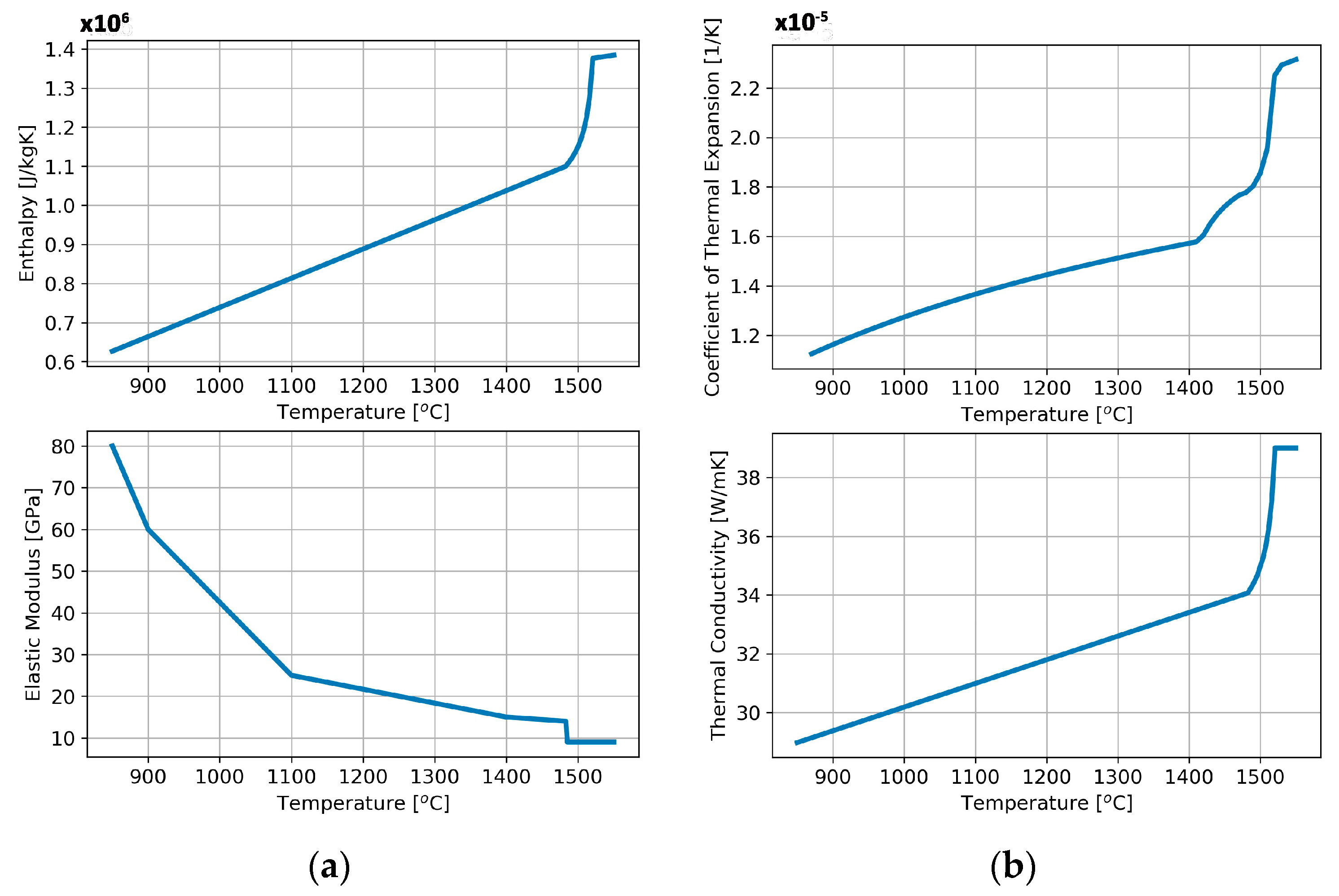
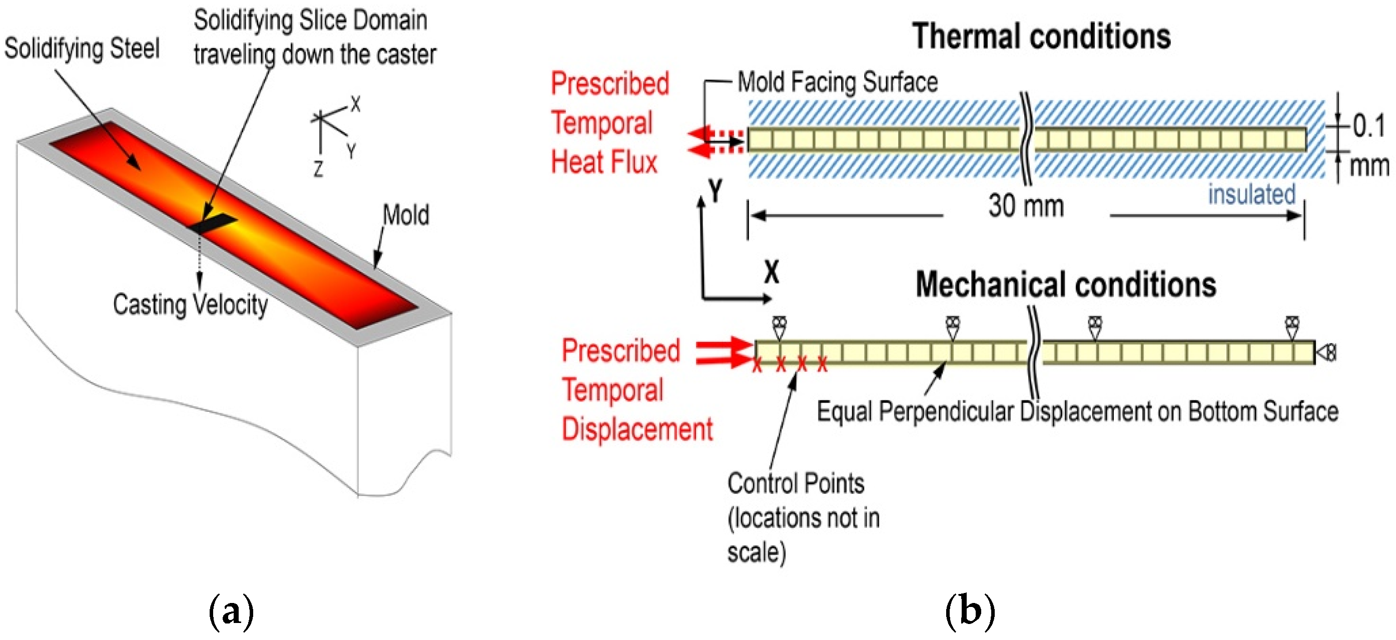
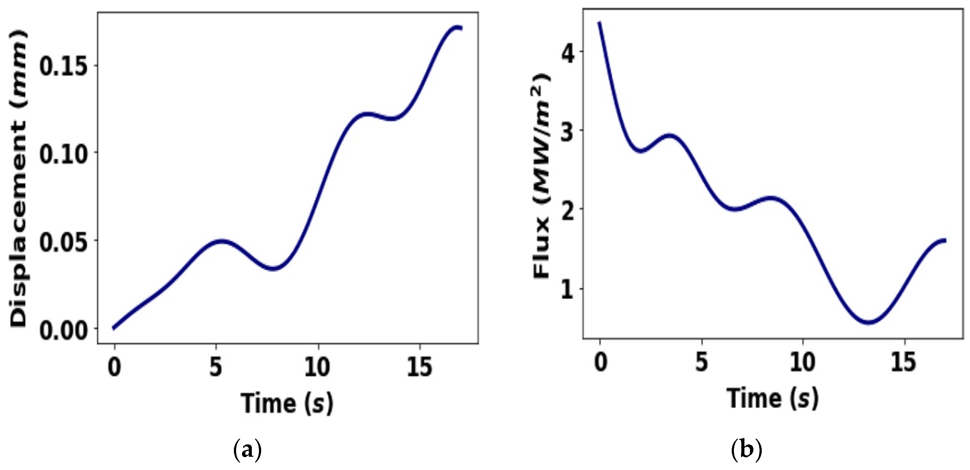
2. Thermo-Mechanical Model of Steel Solidification

We use the modeling results from the existing multiphysics (thermo-mechanical) model [3] with a solidifying slice domain traveling in the Lagrangian frame of reference down the continuous caster to generate training and testing data for the sequential deep learning methods. The governing equation for thermal behavior of the solidifying shell is given in Equation (1)

$$\rho \left(\frac{\partial H}{\partial t}\right)=\nabla \cdot \left(k\nabla T\right),$$

(1)

where k is thermal conductivity, $\rho$ is density, and H is specific enthalpy including the latent heat during phase transformations, such as in solidification and transition from δ-ferrite to austenite. Inertial effects are negligible in solidification problems, so using the quasi-static mechanical equilibrium in Equation (2) as the governing equation is appropriate:

$$\nabla \cdot \mathbf{\sigma }(\mathit{x})+\mathit{b}=0,$$

(2)

where $\mathbf{\sigma }$ is the Cauchy stress tensor and b is the body force density vector. The rate representation of total strain in this thermo-elastic-viscoplastic model is given by Equation (3):

$$\dot{\mathbf{\epsilon }}={\dot{\mathbf{\epsilon }}}_{el}+{\dot{\mathbf{\epsilon }}}_{ie}+{\dot{\mathbf{\epsilon }}}_{th},$$

(3)

where ${\dot{\mathbf{\epsilon }}}_{el},{\dot{\mathbf{\epsilon }}}_{ie},{\dot{\mathbf{\epsilon }}}_{th}$ are the elastic, inelastic, and thermal strain rate tensors, respectively.

At temperatures close to and above the solidification/melting point, steel alloys show significant time- and temperature-dependent plastic behavior, including phase transformations. Kozlowski et al. [21] created a visco-plastic constitutive equation to model the austenite phase of steel, relating inelastic strain to stress, strain rate, temperature, and steel grade via carbon content, Equation (4)

$$\begin{array}{l}{\dot{\overline{\epsilon }}}_{ie}[{\sec }^{-1}]=f_C{\left(\overline{\sigma }[\mathrm{MPa}]-f_1{\overline{\epsilon }}_{ie}|{\overline{\epsilon }}_{ie}{|}^{f2-1}\right)}^{f3}\exp \left(-\frac{Q}{T[\mathrm{K}]}\right)\\ \mathrm{where}:\\ Q=\mathrm{44,465}\\ f_1=130.5-5.128\times {10}^{-3}T[\mathrm{K}]\\ f_2=-0.6289+1.114\times {10}^{-3}T[\mathrm{K}]\\ f_3=8.132-1.54\times {10}^{-3}T[\mathrm{K}]\\ f_C=\mathrm{46,550}+\mathrm{71,400}(\%C)+\mathrm{12,000}{(\%C)}^2\end{array},$$

(4)

where Q is an activation energy constant, $\overline{\sigma }$ (MPa) is Von Mises effective stress, $f_1,f_2,f_3,f_c$ are empirical functions that depend on absolute temperature (K), and %C is carbon content (weight percent) representing steel grade (composition).

Another constitutive model, so called Zhu power law model [22] in Equation (5), was devised to simulate delta ferrite phase with relatively higher creep rate and weaker than austenite phase.

$$\begin{array}{l}{\dot{\overline{\epsilon }}}_{ie}\left(1/\sec .\right)=0.1{\left|\frac{\overline{\sigma }\left(\mathrm{MPa}\right)}{f_{\delta c}(\%C){\left(\frac{T\left({}^{°}\mathrm{K}\right)}{300}\right)}^{-5.52}{(1+1000{\overline{\epsilon }}_{ie})}^m}\right|}^n\\ \mathrm{where}:\\ f_{\delta c}\left(\%C\right)=1.3678\times {10}^4{\left(\%C\right)}^{-5.56\times {10}^{-2}}\\ m=-9.4156\times {10}^{-5}T\left({}^{°}\mathrm{K}\right)+0.3495\\ n=\frac{1}{1.617\times {10}^{-4}T\left({}^{°}\mathrm{K}\right)-0.06166}\end{array}.$$

(5)

The delta-phase model given in Equation (5) is applied in the solid whenever delta-ferrite’s volume fraction is more than 10%, to approximate the dominating influence of the very high-creep rates in the delta-ferrite phase of mixed-phase structures on the net mechanical behavior. While there are sophisticated constitutive models applied in the mushy and liquid zones in the previous works [23,24], in this work, the elastic-perfectly-plastic constitutive model with small yield stress is applied above the solidus temperature Tsol, to enforce negligible strength in those volatile zones. The highly nonlinear constitutive visco-plastic models in Equations (4) and (5) are efficiently integrated at the integration points in UMAT subroutine [3] and linked with Abaqus, which, in turn, solves the coupled thermo-mechanical governing Equations (1) and (2) by the implicit nonlinear finite element solution methodology.

The low carbon steel grade was chosen for this work with 0.09 wt%C, T_sol = 1482.4 °C, and T_liq = 1520.5 °C, whose solidification path is shown in the pseudo-binary iron-carbon phase diagram shown in Figure 1.

Highly temperature-dependent and nonlinear material properties for this steel grade are given in Figure 2a for elastic modulus and enthalpy and in Figure 2b for thermal conductivity and thermal expansion.

The phase fraction and temperature-dependent material properties in Figure 1 and Figure 2 and other interfacial calculations are an integral part of UMAT and other user-defined subroutines, which are programmed and linked with Abaqus to provide a complete multiphysics model of steel solidification on the continuum level [3,8].

Generalized plane strain conditions can realistically recover a full 3D stress state in long objects under thermal loading [3,4], such as in continuous caster in Figure 3a with the considerable length and width. The slice domain in Figure 3b travels down the mold with casting velocity in a Lagrangian frame of reference. It consists of a single row of 300 coupled thermo-mechanical generalized plane strain elements with 602 nodes, which provide generalized plane strain condition in axial (z-direction). In addition, a second generalized plane strain condition was imposed in the y direction by coupling the vertical displacements of all nodes along the bottom edge of the domain. Time-dependent profiles of thermal fluxes leaving the chilled surface on the left side of the domain and their displacement due to mold taper and other interactions with the mold provide the solidifying slice domain’s thermal and mechanical boundary conditions. These profiles’ temporal variations are inputs for the sequence deep learning methods, while the calculated temperature and stress histories are their targets (labels).

3. Deep Learning Models

Deep learning is a subset of machine learning. Deep learning models consist of neural networks, a hierarchical organization of layers of neurons connected to other neurons’ layers.

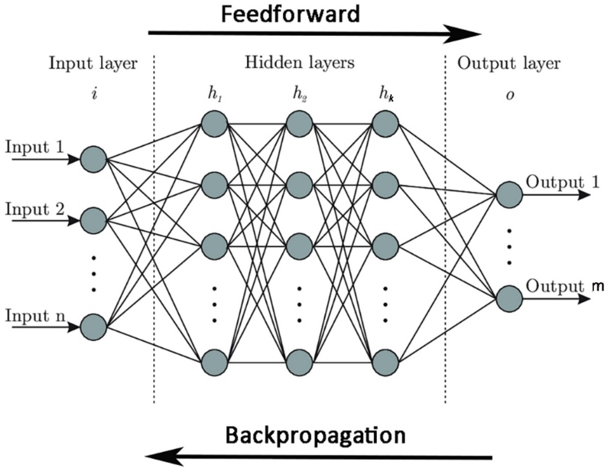
3.1. Dense Feedforward Neural Network

As shown in Figure 4, the most straightforward neural network, the so-called dense feedforward neural network, comprises linked layers of neurons that calculate predictions based on input data.

The layers with neurons feed information forward to other layers based on the received input, and this forms a complex network that learns with some feedback mechanism. The number of hidden layers, i.e., the layers in between input and output layers, defines a neural network’s deepness. Neurons of successive layers are connected through associated weights and biases W and b. The output ${\widehat{\mathit{Y}}}^{[l]}$ for a layer l is calculated as:

$$\begin{array}{l}{\mathit{Z}}^{[l]}={\mathit{W}}^{[l]}{\mathit{Z}}^{[l-1]}+{\mathit{b}}^{[l]}\\ {\widehat{\mathit{Y}}}^{[l]}=f^{[l]}({\mathit{Z}}^{[l]})\end{array},$$

(6)

where W^[l](n_l × n_l−1) and b^[l] (n_l−1 × 1) are matrix of weights and vector of biases, respectively which are updated after every training pass. f^[l] is the activation function that transforms Z into output for every neuron in the layer l. Activation functions in neural networks are nonlinear functions such as Rectified Linear Unit (ReLu), Sigmoid, and Hyperbolic Tangent. They enable the neural network to learn almost any complex functional relationship between inputs and outputs. At the end of each feed-forward pass, the loss function L compares the predictions to the targets by calculating a loss value that measures how well the network’s predictions match what was expected. Then, in a backpropagation process, the optimizer minimizes loss value iteratively with gradient descent in Equation (7) and other similar optimization techniques. The gradients of loss function L are calculated with respect to the weights in the last layer, and the weights are updated for each node before the same process is done for the previous layer and backward until all of the layers have had their weights adjusted. Then, a new k iteration with forward propagation starts again. After a reasonable amount of iterations, the series W^k should converge toward the minimum loss value location. The parameter γ is called the learning rate.

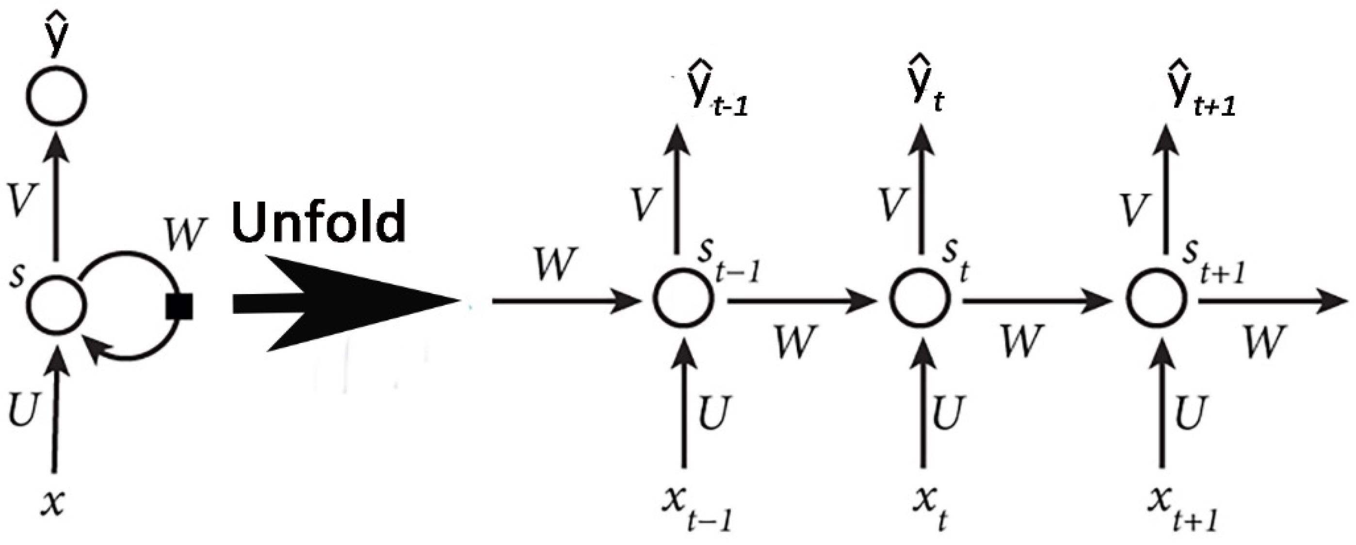
3.2. Recurrent Neural Networks

In a feedforward neural network, we assume that all inputs (and outputs) are independent of each other. However, we want to predict the next value in a sequence for many deep learning tasks, such as a word in a sentence, by knowing which words came before it. The most known sequence neural network is the family of recurrent neural networks (RNN). They are called recurrent because they perform the same task for every element of a sequence, with the output being dependent on the previous computations. Sequence learning predicts for a given input sequence $x_0,\dots ,x_T$ the matching outputs ${\widehat{y}}_0,\dots ,{\widehat{y}}_T$ at each time step while minimizing the loss function L between predictions ${\widehat{y}}_0,\dots ,{\widehat{y}}_T$ and actual targets $y_0,\dots ,y_T$. The diagram in Figure 5 shows RNN being unfolded in time into a full network for an entire sequence and is described by the propagation expressions in Equation (7).

$$\begin{array}{l}{\mathit{s}}_t=f(\mathit{U}{\mathit{x}}_t+\mathit{W}{\mathit{s}}_{t-1}+\mathit{b})\\ {\widehat{\mathit{y}}}_t=\mathit{V}{\mathit{s}}_t+\mathit{c}\end{array}.$$

(7)

${\mathit{s}}_t$ is the hidden state at time step t, also known as the “memory” of the recurrent network since it captures information about what happened in all the previous time steps. It is calculated from the previous hidden state and the input at the current step represented by W (hidden-to-hidden) and U (input-to-hidden) weight connections, respectively, f is the activation function, and b is a bias. Output prediction at time step t is calculated from ${\mathit{s}}_t$ using V (hidden-to-output) weights and c bias. Similarly, to the dense feedforward network, all weights and biases are updated from their loss gradients by backpropagations. However, recurrent neural networks often consist of very deep computational graphs repeatedly (recurrently) applying the identical operation at each time step of a long-time sequence. This may cause the vanishing or exploding gradient problems during backpropagation and makes it challenging to train long sequence data with RNNs. To address the vanishing gradient problems of traditional RNN, the long short-term memory (LSTM) [25] and gated recurrent unit (GRU) [26] are devised. Hidden state (memory) cells in the LSTM and GRU advanced recurrent neural networks are designed to dynamically “forget” some old and unnecessary information via select gated units that control the flow of information inside a memory cell, thus avoiding multiplication of a long sequence of numbers during temporal backpropagation. GRU has a simpler gated unit architecture than LSTM and generally learns faster than LSTM. A recent work [19] has shown that GRU’s formulation is less prone to overfitting in materially non-linear sequence learning and allows faster training due to the smaller number of trainable parameters. A comprehensive mathematical overview of LSTM and GRU networks can be found here [27].

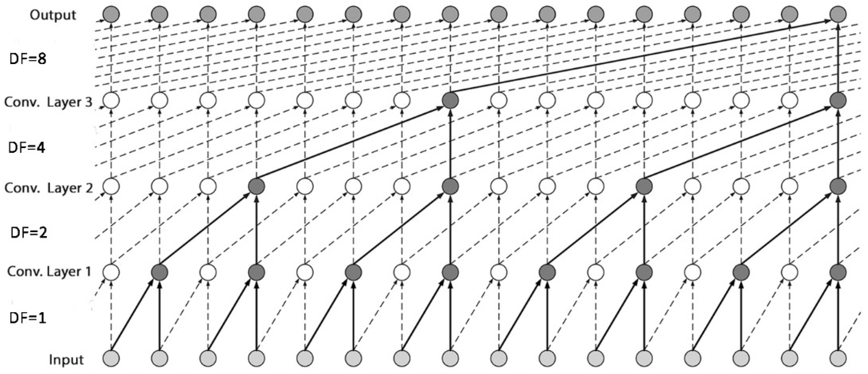
3.3. Temporal Convolutional Neural Network

The temporal convolutional network (TCN) is a variant of Convolutional Neural Networks particularly adept for sequence learning tasks. The two-dimensional (standard) version of Convolutional Neural Networks (CNN) is generally considered the best deep learning model available today for computer vision tasks. Convolution is sliding a smaller matrix (known as a kernel or filter) over a larger matrix representing an image. At each run, we do an element-wise multiplication of the two matrix elements and add them. The kernel slides to another portion of the image matrix until the whole image is convoluted, and a feature map corresponding to a particular kernel is computed. The gradients of the loss function with respect to kernel weights are then calculated in a backpropagation process, and the weights are updated similar to dense feedforward artificial neural networks. There are many kernels in a typical computer vision CNN such as geometric shapes, edges, distribution of colors, etc. This makes these networks very robust in image classification and other similar data that contain 2D-spatial properties. TCN uses a one-dimensional version of CNN where the kernel slides along a single dimension, i.e., time. In these so-called casual convolutions, an output at time t is convoluted only with elements from time t and earlier in the previous layer, as shown in Figure 6. No information from the future is propagated into the past. To produce an output of the same length as the input layer, zero padding of length (kernel size − 1), is added to keep subsequent layers the same size as previous ones. Multiple 1D convolutional layers are typically stacked on top of each other in order to learn from the previous time steps.

The dilation factor (DF), or receptive field enlargement with gaps in entries of subsequent convolution layers, is increased exponentially to achieve large receptive field sizes. Since TCN does not perform recurring calculations, it is more robust with respect to vanishing and exploding gradients than any RNN network. It is more computationally and memory efficient. More detailed information about TCN can be found in [28].

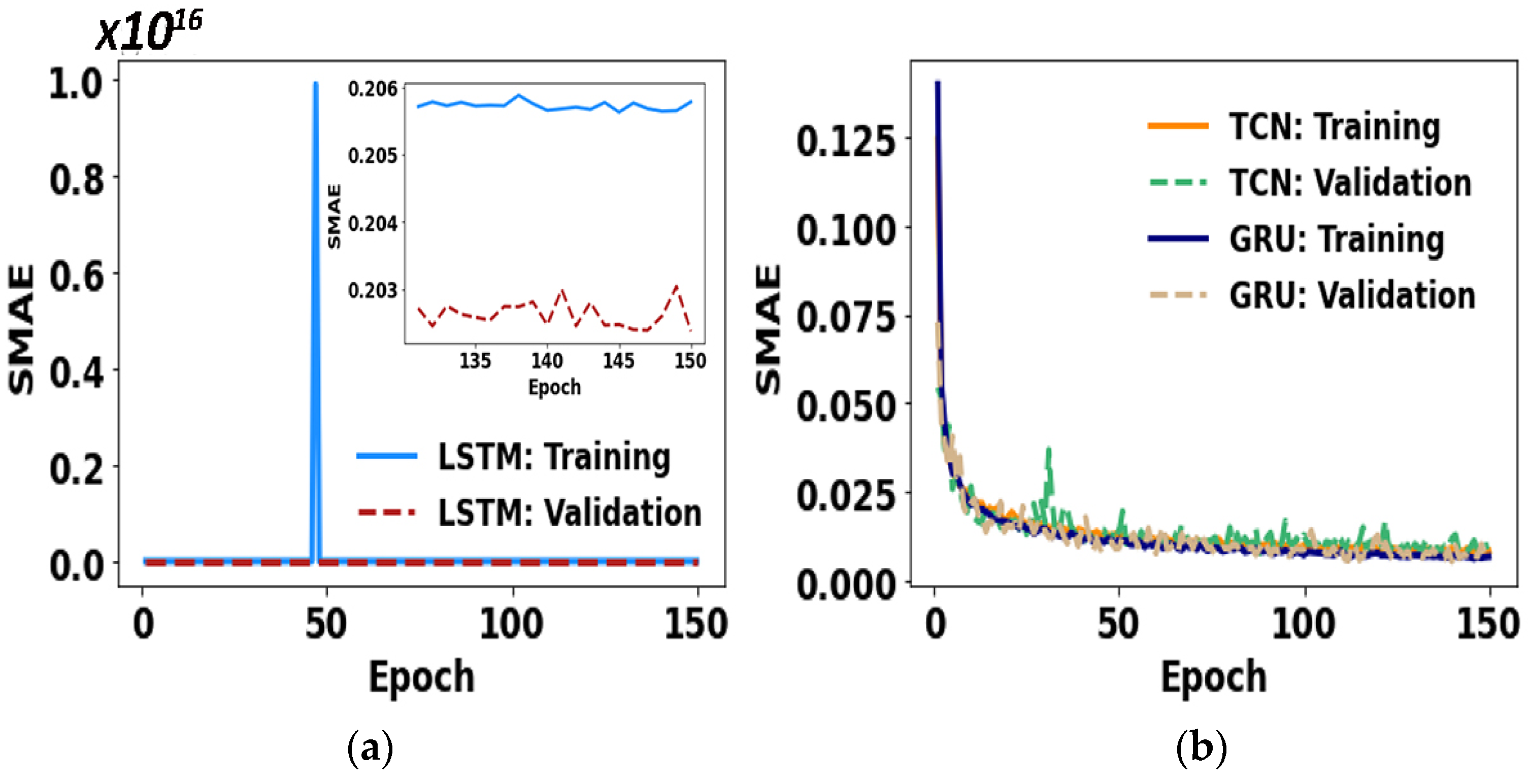
4. Results and Discussion

Instantaneous heat flux profile on the chilled surface is essential for the multiphysics analysis that drives the solidifying shell’s transient heat transfer. Similarly, the chilled solidifying shell surface’s displacement profile due to the mechanical contact and interactions with the mold surface is an important boundary condition for mechanical analysis. Based on a variation of the time histories of heat flux and displacement boundary conditions, the multiphysics model of solidifying slice from Chapter 2 is run for 17 s of simulation time that the slice spends solidifying in the mold. Thus, we generate temperature and stress histories at the four spatial control points along the slice’s bottom edge at the chilled surface and 1, 2, and 3 mm in the domain interior (see Figure 3), which are used as targets (labels) for the sequence deep learning methods. The points are chosen on those locations since casting quality depends on the solidification conditions on the chilled surface and its subsurface. It is known from the steel plant observations that the thermal flux has an overall decaying profile due to transient heat transfer, while the displacement profile has an increasing trend due to mold taper. After having several temporal points defined randomly within ranges of expected profile values, a radial basis interpolation with Gaussian function is used to connect (interpolate) the points and to emulate additional fluctuations and data noise observed in the actual flux and displacement profiles due to sudden changes in contact conditions and interfacial heat transfer between mold and steel surfaces. Many thousands of these thermal and displacement variations provided all possible scenarios that the solidifying shell encounters on its chilled surfaces while traveling down the caster, as well as a sufficient number of data samples generated for deep learning. One such test input data sample with displacement and heat flux profiles is given in Figure 7.

Figure 8 shows the schematic diagram of a training process in sequence learning in this work. The modeling database provides inputs for sequence neural networks and temperature and stress sequences, i.e., labels (targets). The loss function compares predictions from the neural network to the labels and calculates a loss value. The optimizer minimizes the loss value and updates the weights of the network iteratively, as explained earlier.

The three deep learning models have a comparable number of approximately 3.5 million total trainable parameters, such as entries in W, U, V, b, and c weight and bias matrices in Figure 5 that connect a multitude of nodes and layers of the recurrent neural networks, and with each network consisting of 3 hidden layers. This provided an optimum between computational cost and minimization of errors. The input and target data for over 14,000 samples, each with 100 time steps, are generated using high-throughput computing capabilities of several nodes of the high-performance computing cluster called iForge at the National Center for Supercomputing Applications at the University of Illinois. Approximately, 80% of the generated data samples are randomly selected for training with the LSTM, GRU, and TCN sequence deep learning methods, discussed in Section 3, on an iForge’s computing node equipped with GPUs using Keras [29] with TensorFlow backend. The remaining 20% of the data is set aside for testing and validation. Figure 9 depicts an example of each sequence learning model’s convergence plots for 150 training epochs in terms of scaled mean absolute error (SMAE).

The training of the LSTM sequence learning model is generally extremely unstable, as can be seen in Figure 9. This is not the case with GRU and TCN. Both deep learning models provided accurate qualitative and quantitative results, with slight variations in the SMAE and steady converging. Figure 10 shows ground-truth stress and temperature results calculated for the four control points by the multiphysics model and the corresponding sequence learning predictions from the neural networks for the test input sample in Figure 7, which was never trained by any deep learning network.

The GRU and TCN deep learning models almost perfectly predicted the highly complex and coupled multiphysics thermo-mechanical phenomena of steel solidification with multiple visco-plastic constitutive laws, generating tensile and compressive residual stresses on the chilled surface and its subsurface. These stresses and strains are responsible for most cracks and other defects initiating in the continuous casting of steel [4]. The LSTM model, on the other hand, only roughly predicted the temperatures and stresses histories mainly due to its limited capabilities to cope with long sequences of data such as here with 100 time steps. We have inferred results from many other test samples, which again were never trained by the deep learning networks. Every time the GRU and TCN models were able to accurately predict the stress and temperature histories. This is summarized in Figure 11 in terms of average SMAE with its standard deviation for all the testing samples. The LSTM-based model has the highest error values among the models, while the GRU- and TCN-based models have similar error values. However, the TCN model was eight times faster in training than the GRU-based model due to its convolutional algorithm that avoids recurrent calculations and generally much better utilizes the GPU hardware.

5. Conclusions

We have applied and compared the three types of deep sequence learning methods, short-term memory (LSTM), gated recurrent unit (GRU), and temporal convolutional network (TCN), to a multiphysics model of steel solidification. We have found that only the TCN- and GRU-based models could learn and gain enough artificial intelligence to accurately reproduce the extremely complex multiphysics behavior of a solidifying steel domain moving in a continuous caster. At the same time, the TCN-based model is also significantly more computationally efficient. Moreover, once appropriately trained on a high-end computing system with sufficient sequenced data generated from classical multiphysics finite element simulations, the model’s trained weights and biases can be transferred to any low-end computer. Thus, the deep learning models developed in this work can almost instantly produce (inference) good quality results for unseen input data on laptops and without any modeling software. Finally, it is worth pointing that the deep learning methodology developed here is not confined to the slice domain or the constitutive models used in this work. Still, it is readily applicable to other solidification domains and constitutive models. These and other similar Artificial Intelligence (AI)-based surrogate data-driven methods will open the door for future highly accelerated multiphysics modeling, design, optimization, and process predictions in steel solidification and other complex manufacturing processes.

References

1. Lee, J.-E.; Yeo, T.-J.; Hwan, O.K.; Yoon, J.-K.; Yoon, U.-S. Prediction of cracks in continuously cast steel beam blank through fully coupled analysis of fluid flow, heat transfer, and deformation behavior of a solidifying shell. Metall. Mater. Trans. 2000, 31, 225–237. [Google Scholar] [CrossRef]
2. Teskeredžić, A.; Demirdžić, I.; Muzaferija, S. Numerical method for heat transfer, fluid flow, and stress analysis in phase-change problems. Numer. Heat Transf. Part B Fundam. 2002, 42, 437–459. [Google Scholar] [CrossRef]
3. Koric, S.; Thomas, B.G. Efficient thermo-mechanical model for solidification processes. Int. J. Numer. Methods Eng. 2006, 66, 1955–1989. [Google Scholar] [CrossRef]
4. Li, C.; Thomas, B.G. Thermomechanical finite-element model of shell behavior in continuous casting of steel. Metall. Mater. Trans. B 2004, 35, 1151–1172. [Google Scholar] [CrossRef]
5. Abaqus/Standard User’s Manual Version 2019; Simulia Dassault Systèmes: Providence, RI, USA, 2019.
6. Koric, S.; Hibbeler, L.C.; Thomas, B.G. Explicit coupled thermo-mechanical finite element model of steel solidification. Int. J. Numer. Methods Eng. 2009, 78, 1–31. [Google Scholar] [CrossRef] [Green Version]
7. Koric, S.; Thomas, B.G.; Voller, V.R. Enhanced Latent Heat Method to Incorporate Superheat Effects into Fixed-Grid Multiphysics Simulations. Numer. Heat Transf. Part B Fundam. 2010, 57, 396–413. [Google Scholar] [CrossRef]
8. Koric, S.; Hibbeler, L.C.; Liu, R.; Thomas, B.G. Multiphysics Model of Metal Solidification on the Continuum Level. Numer. Heat Transf. Part B Fundam. 2010, 58, 371–392. [Google Scholar] [CrossRef]
9. Zappulla, M.L.; Cho, S.-M.; Koric, S.; Lee, H.-J.; Kim, S.-H.; Thomas, B.G. Multiphysics modeling of continuous casting of stainless steel. J. Mater. Process. Technol. 2020, 278, 116469. [Google Scholar] [CrossRef]
10. Zhang, S.; Guillemot, G.; Gandin, C.-A.; Bellet, M. A Partitioned Solution Algorithm for Concurrent Computation of Stress–Strain and Fluid Flow in Continuous Casting Process. Met. Mater. Trans. A 2021, 1–18. [Google Scholar] [CrossRef]
11. Cai, L.; Wang, X.; Wei, J.; Yao, M.; Liu, Y. Element-Free Galerkin Method Modeling of Thermo-Elastic-Plastic Behavior for Continuous Casting Round Billet. Met. Mater. Trans. B 2021, 1–11. [Google Scholar] [CrossRef]
12. Huitron, R.M.P.; Lopez, P.E.R.; Vuorinen, E.; Jentner, R.; Kärkkäinen, M.E. Converging criteria to characterize crack susceptibility in a micro-alloyed steel during continuous casting. Mater. Sci. Eng. A 2020, 772, 138691. [Google Scholar] [CrossRef]
13. Li, G.; Ji, C.; Zhu, M. Prediction of Internal Crack Initiation in Continuously Cast Blooms. Met. Mater. Trans. B 2021, 1–15. [Google Scholar] [CrossRef]
14. Rong, Q.; Wei, H.; Huang, X.; Bao, H. Predicting the effective thermal conductivity of composites from cross sections images using deep learning methods. Compos. Sci. Technol. 2019, 184, 107861. [Google Scholar] [CrossRef]
15. Goli, E.; Vyas, S.; Koric, S.; Sobh, N.; Geubelle, P.H. ChemNet: A Deep Neural Network for Advanced Composites Manufacturing. J. Phys. Chem. B 2020, 124, 9428–9437. [Google Scholar] [CrossRef] [PubMed]
16. Abueidda, D.W.; Koric, S.; Sobh, N.A. Topology optimization of 2D structures with nonlinearities using deep learning. Comput. Struct. 2020, 237, 106283. [Google Scholar] [CrossRef]
17. Kollmann, H.T.; Abueidda, D.W.; Koric, S.; Guleryuz, E.; Sobh, N.A. Deep learning for topology optimization of 2D metamaterials. Mater. Design 2020, 196, 109098. [Google Scholar] [CrossRef]
18. Spear, A.D.; Kalidindi, S.R.; Meredig, B.K.; Le Graverend, A.J.-B. Data driven materials investigations: The next frontier in understanding and predicting fatigue behavior. JOM 2018, 70, 1143–1146. [Google Scholar] [CrossRef] [Green Version]
19. Mozafar, M.; Bostanabad, R.; Chen, W.; Ehmann, K.; Cao, J.; Bessa, M. Deep learning predicts path-dependent plasticity. Proc. Natl. Acad. Sci. USA 2019, 116, 26414–26420. [Google Scholar] [CrossRef] [Green Version]
20. Abueidda, D.W.; Koric, S.; Sobh, N.A.; Sehitoglu, H. Deep learning for plasticity and thermo-viscoplasticity. Int. J. Plast. 2021, 136, 102852. [Google Scholar] [CrossRef]
21. Kozlowski, P.F.; Thomas, B.G.; Azzi, J.A.; Wang, H. Simple constitutive equations for steel at high temperature. Met. Mater. Trans. A 1992, 23, 903–918. [Google Scholar] [CrossRef]
22. Zhu, H. Coupled Thermo-Mechanical Finite-Element Model with Application to Initial Solidification. Ph.D. Thesis, The University of Illinois at Urbana-Champaign, Urbana, IL, USA, May 1996. [Google Scholar]
23. Fachinotti, V.D.; Le Corre, S.; Triolet, N.; Bobadilla, M.; Bellet, M. Two-phase thermo-mechanical and macrosegregation modelling of binary alloys solidification with emphasis on the secondary cooling stage of steel slab continuous casting processes. Int. J. Numer. Methods Eng. 2006, 67, 1341–1384. [Google Scholar] [CrossRef] [Green Version]
24. Zhu, J.Z.; Guo, J.; Samonds, M.T. Numerical modeling of hot tearing formation in metal casting and its validations. Int. J. Numer. Methods Eng. 2011, 87, 289–308. [Google Scholar] [CrossRef]
25. Hochreiter, S.; Schmidhuber, J. Long Short-Term Memory. Neural Comput. 1997, 9, 1735–1780. [Google Scholar] [CrossRef]
26. Cho, K.; van Merrienboer, B.; Gulcehre, C.; Bahdanau, D.; Bougares, F.; Schwenk, H.; Bengio, Y. Learning Phrase Represen-tations using RNN Encoder-Decoder for Statistical Machine Translation. arXiv 2014, arXiv:1406.1078. [Google Scholar]
27. Pattanayak, S. Pro Deep Learning with TensorFlow, A Mathematical Approach to Advanced Artificial Intelligence in Python, 1st ed.; Apress Media LLC, Springer Media: New York, NY, USA, 2017; pp. 262–277. [Google Scholar]
28. Alla, S.; Adari, S.K. Beginning Anomaly Detection Using Python-Based Deep Learning, 1st ed.; Apress Media LLC, Springer Media: New York, NY, USA, 2019; pp. 257–282. [Google Scholar]
29. Keras, Chollet, François. Available online: https://github.com/keras-team/keras (accessed on 8 February 2021).
Figure 1. Pseudo-binary iron-carbon phase diagram with solidification path for 0.09 wt%C low carbon steel grade.
Metals 11 00494 g001
Figure 2. Temperature dependent material properties for 0.09 wt%C steel grade: (a) elastic modulus and enthalpy and (b) thermal conductivity and thermal expansion.
Metals 11 00494 g002
Figure 3. (a) Continuous caster with solidifying slice finite element domain and (b) thermal and mechanical boundary conditions.
Metals 11 00494 g003
Figure 4. Dense feedforward deep neural network.
Metals 11 00494 g004
Figure 5. Recurrent neural network with its unfolding in time calculations.
Metals 11 00494 g005
Figure 6. Temporal convolutional neural network.
Metals 11 00494 g006
Figure 7. Example of a testing input data sample: (a) displacement profile and (b) flux profile.
Metals 11 00494 g007
Figure 8. Training process in sequence deep learning.
Metals 11 00494 g008
Figure 9. Convergence history: (a) LSTM and (b) GRU and TCN.
Metals 11 00494 g009
Figure 10. Output results, ground-truth, and deep learning predictions for the 4 control points, corresponding to the testing input sample in Figure 7.
Metals 11 00494 g010
Figure 11. Training times and testing scaled mean absolute error (SMAE).
Metals 11 00494 g011
Publisher’s Note: MDPI stays neutral with regard to jurisdictional claims in published maps and institutional affiliations.