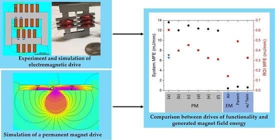
Actuating a Magnetic Shape Memory Element Locally with a Set of Coils

Abstract

The local actuation of a magnetic shape memory (MSM) element as used in an MSM micropump is considered. This paper presents the difference between an electromagnetic driver and a driver that uses a rotating permanent magnet. For the magnetic field energy of the permanent magnetic drive, the element takes in a significant stray field. In a particular case, energy reduction was 12.7 mJ. For an electromagnetic drive with an identical size of the MSM element, the total magnetic field energy created by the system was 2.28 mJ. Attempts to experimentally nucleate twins in an MSM element by energizing an electromagnetic drive failed even though the local magnetic field exceeded the magnetic switching field. The energy variation is an order of magnitude smaller for the electromagnetic drive, and it does not generate the necessary driving force. It was assumed in previous work that the so-called magnetic switching field presents a sufficient requirement to nucleate a twin and, thus, to locally actuate an MSM element. Here, we show that the total magnetic field energy available to the MSM element presents another requirement.

1. Introduction

Progress in modern technology depends upon novel materials with specific physical and functional properties. Some intermetallic alloys exhibit the shape memory effect, where the material experiences a shape change from an external stimulus such as temperature, magnetic field, and mechanical stress (e.g., [1,2,3]). Magnetic shape memory (MSM) alloys exhibit shape change resulting from magnetic field. Single crystal MSM alloy exhibits a large stroke and short actuation time with the ability to change its size and shape several million times. Essentially, the material operates as a metallic muscle controlled by the variation of a magnetic field. Ni-Mn-Ga exhibits a martensite phase with highly mobile twin boundaries. Upon the application of mechanical stress or a magnetic field, the twin domains reorient and enable high magnetic-field-induced strain. MSM alloys are considered for applications in microactuators, strain sensors [4], energy harvesters [5,6], and micropumps [7,8,9].

In a uniform magnetic field, the MSM element deforms by extending and contracting uniformly in the bulk, as would a piezoelectric element [10]. In contrast, a localized magnetic field causes a localized shrinkage in the MSM element, which can be moved along with the localized magnetic field [7]. Rotation of the localized field moves a shrinkage through an MSM element [11]. The motion of the shrinkage along the element can be used to build a pump in a similar manner to the esophageal contractions that mammals use to swallow food [7].

In previous work, the rotating magnetic field has been provided by the rotation of a diametrically magnetized permanent magnet, where a micromotor spun the magnet. Micromotors are large in comparison to an MSM sample and have moving parts prone to failure. In lieu of actuating the shrinkage with a physically rotating magnet, this study considers the advancement of a localized magnetic field using a miniature electromagnet with a plurality of magnetic poles. Previously, to consider the actuation of an MSM sample by localized electromagnetic coils, Smith et al. physically repositioned the poles of an electromagnet [12]. The authors found that a locally twinned region formed at the magnetic pole tips. In [13], we created a motionless magnetic driver in a device with multiple magnetic poles arranged in a row. Individual poles were energized with a strong magnetic field by compressing a magnetic field through two coils in opposition adjacent to a soft ferromagnetic pole. Changing the polarity of the coils energized other poles and advanced a magnetic field. The shrinkage formed on the MSM element near the pole tips. However, the spacing between poles was too coarse to move the deformed region.

In this paper, we present an electromagnetic drive with two rows of magnetic poles, similar to linear motor yokes, which are staggered across the MSM element. Each pole can be energized individually and sequentially to approximate a moving vertical field along the MSM element. A device was built to test the effect of the pulsing electromagnetic drive upon an MSM element. Along with physical results, magnetic models using finite element method magnetics (FEMM) were created. The material and magnetic behavior is compared to that known when driven by a rotating rare earth Nd-Fe-B magnet.

2. Materials and Methods

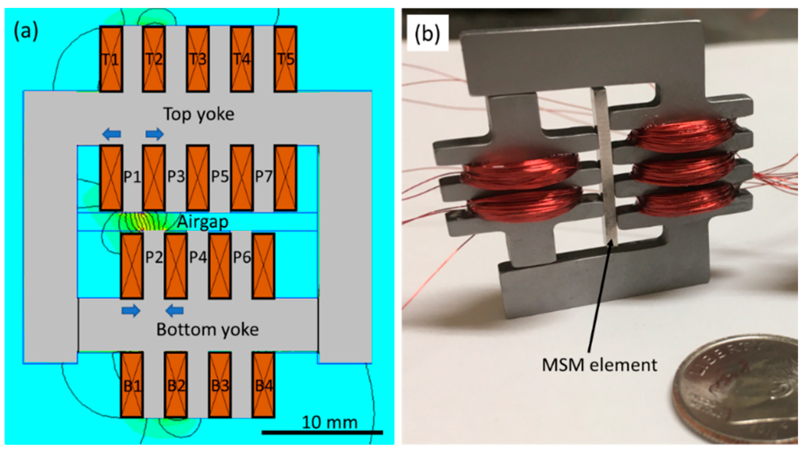
2.1. Device Design

The magnetic yokes were machined as shown in Figure 1 out of a 3.0 mm thick plate of Fe-Co (Vacoflux 50). The material is magnetically soft and supports 2.3 T at saturation [14]. The yoke was composed of a top and bottom yoke that interfaced via a friction fit. The bottom yoke had three poles and the top yoke had four poles. The bottom yoke slid into the top yoke. The two yokes had poles juxtaposed to each other. In Figure 1a, the yokes are separated by an air gap. The poles (P1–P7) were magnetized by the bottom coils, B1–B4, and the top coils T1–T5. Figure 1a shows the flux pattern when P1 and P2 are actuated with magnetic flux flowing upward.

Each side of the yoke had an inner row of poles and an outer row of poles. The outer poles were simply for coil containment when winding. Upon actuation, the magnetic circuit guided the vast majority of magnetic flux through the inner poles. The inner width of the yoke was 20 mm, which was designed to accommodate an MSM element. The edges were deburred by sandblasting such that coils could be wound directly onto the yokes. The coil wire had a polyamide coated and a diameter of 0.13 mm (36 AWG). Figure 1b shows the yokes with only five coils, while for the experiments, four coils were added outside of the outermost poles in each row. Each coil in the drive had 200 turns. The coils were wound on a machinist lathe.

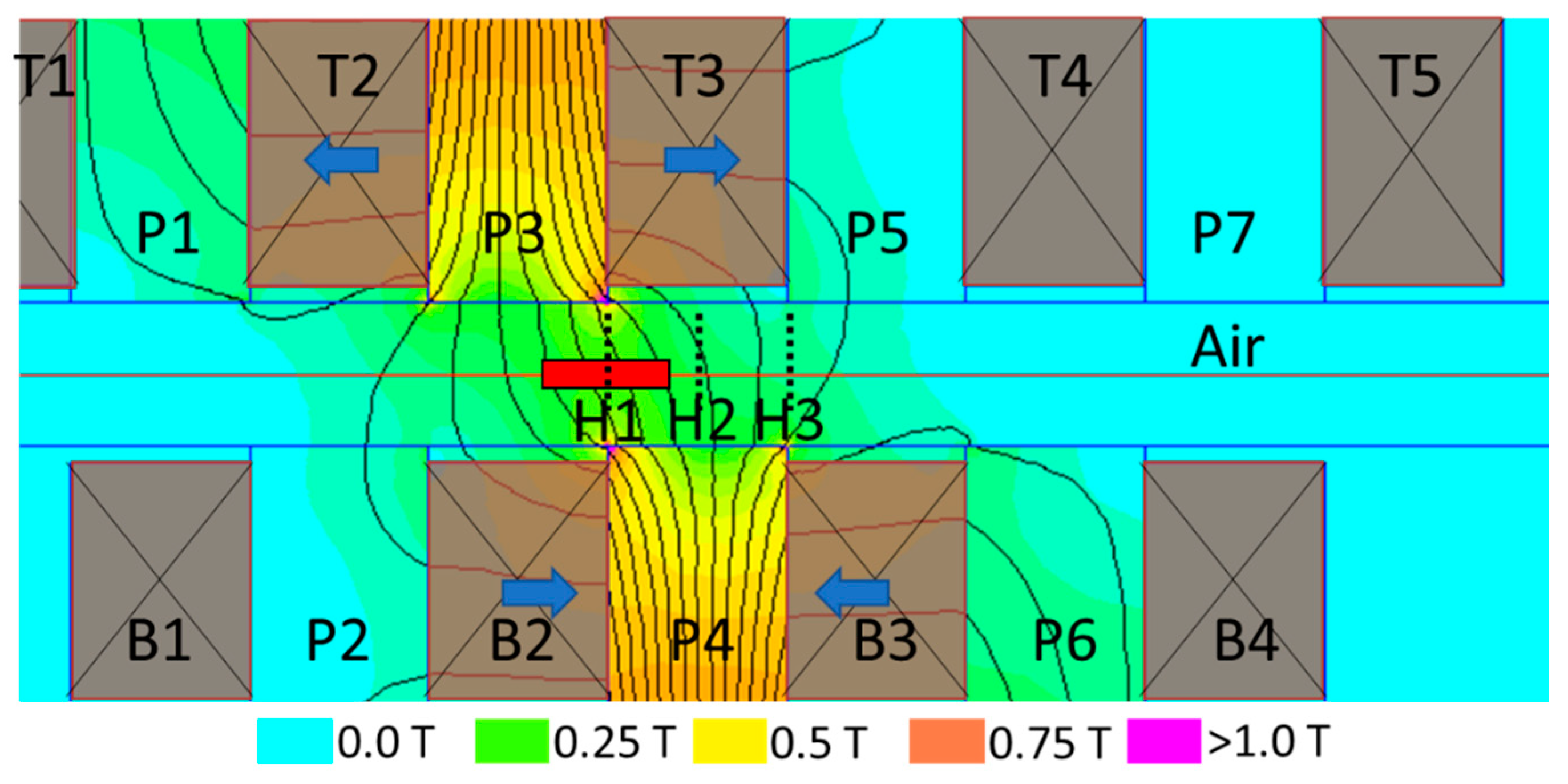
2.2. Magnetic Circuits and Magnetic Field Propagation

To create and move the vertical magnetic field patterns, circuits were sequentially energized. In Figure 1a, for example, coils B1 and B2 were energized in opposition thereby creating a North pole to form at P2. Coils T1 and T2 were opposed and with polarity opposite to the B1 and B2 coils. Therefore, P1 becomes a South pole. The magnetic field streamed from the North pole (P2) to the South pole (P1) across the air gap.

Five circuits were identified as suitable to induce and advance a strong vertical magnetic field. The mechanism considered advanced the field by one pole pitch, although the mechanism could have been extended in either direction. The circuit was numbered according to the position in sequence. The circuits were described by the energized, opposed electrical coil pair (B2, B3) and the pole direction they cause at the airgap (N or S). The circuits were:

• (B2, B3) N, (T2, T3) S
• (B2, B3) N, (T2, T4) S
• (B2, B3) N, (T3, T4) S
• (B2, B4) N, (T3, T4) S
• (B3, B4) N, (T3, T4) S which begins the next elementary sequence.

2.3. Magnetic Measurements

We measured the device induction in the air gap as a function of coil current. The gap was 1.4 mm, which corresponded to the thickness of the MSM element used in this study. Each circuit was energized using an Uno microcontroller (Arduino, Somerville, MA, USA), which controlled an 8 channel 5 V optocoupled relay board (Sunfounder, Shenzhen, China). Ten millisecond pulses were applied and were nearly rectangular in the oscilloscope. The magnetic field was measured using a GM08 gaussmeter (Hirst Magnetic Instruments, Falmouth, UK) with a transverse Hall probe with a 1.5 mm wide Hall sensor. The measured Hall sensor location is indicated by the red box in Figure 2. For the measured circuits 1, 2, and 3, the hall probe was at locations H1, H2, and H3, respectively.

Circuits 1, 2, and 3 were characterized by measuring the magnetic field and current at 1 V increments. The circuit was powered with a 30 V, 5 A power supply (BK Precision, Yorba Linda, CA, USA) and measured the current with a shunt resistor. An Analog Discovery 2 oscilloscope (Digilent, Pullman, WA, USA) was used to collect these data.

2.4. Actuation with MSM Element

A single crystal 10 M Ni₅₀Mn₂₈.₅Ga₂₁.₅ MSM element was used, which was manufactured at Boise State University [15]. The MSM element measured 1.4 mm × 2.0 mm × 20 mm. The faces were cut parallel to {100} crystallographic planes. The element was electropolished in a 1:3 14 M Nitric acid in ethanol solution. The element was compressed along the 20 mm dimension such that the crystallographic c-axes, which coincided with the direction of easy magnetization, were all aligned in the horizontal direction (Parent variant) throughout the entire element. The sample faces were mechanically ground and then finely polished using 0.3 µm diamond suspension for optical analysis. A twin domain, where the c-axis was aligned along the short dimension of the element, was mechanically induced into a portion of the element with calipers such that the volume fraction of the twin was approximately 15% following Ref. [12]. Then, the sample was fixed in this configuration to a glass coverslip with double-sided tape. The MSM element was actuated by circuits described in Section 2.2 and Section 2.3 with an electrical current of 1 A on each coil.

The MSM element was inserted into the drive. The entire drive was placed on the stage of an optical microscope with polarized illumination. Then, circuits described in 2.2 were applied to the MSM element. Video analysis and still micrography were used to measure the twin boundary motion at the expected shrinkage location.

3. Finite Element Analysis

The change of shape and magnetization properties of the MSM material causes several effects on the MSM actuator such as a change of the inductance and magnetic permeability. Commercial finite element analysis tools are not capable of simultaneously calculating the magnetic field, mechanical stress, and resulting shape change in MSM actuators. Integrated magneto-mechanical material models are not commercially available [16,17]. Furthermore, the commonly used 10 M phase of Ni-Mn-Ga has nearly uniaxial anisotropy with a first-order uniaxial constant of K₁(283 K) = 2.0 × 10⁵ J/m³ [18]. For example, a volume of 2.0 mm³ twinned section in the MSM element would change the magnetocrystalline anisotropy energy of the MSM element by about 0.4 mJ.

In our model, the parent variant had a magnetic permeability of μ_r = 2 in the vertical direction and 40 in the horizontal direction [19]. The twin was the opposite and had its axis of easy magnetization in the vertical direction (μ_r = 40). All FEMM simulations use an energization current of 1 A/coil, producing a field in the coil in the direction indicated by arrows.

In this model, the magnetic permeability was assumed to be constant and not depend upon the field strength. Simulation of the dynamical response of the material is not straightforward. Provided a sufficiently strong magnetic field, the material switches to become twinned. Once the twin is formed, the twin becomes a low-reluctance “short” in the magnetic circuit. The position of the “short” dictates the shape of the resultant circuit. The dynamic variation of the magnetic structure was accounted for by simulating instances before and after the switching event.

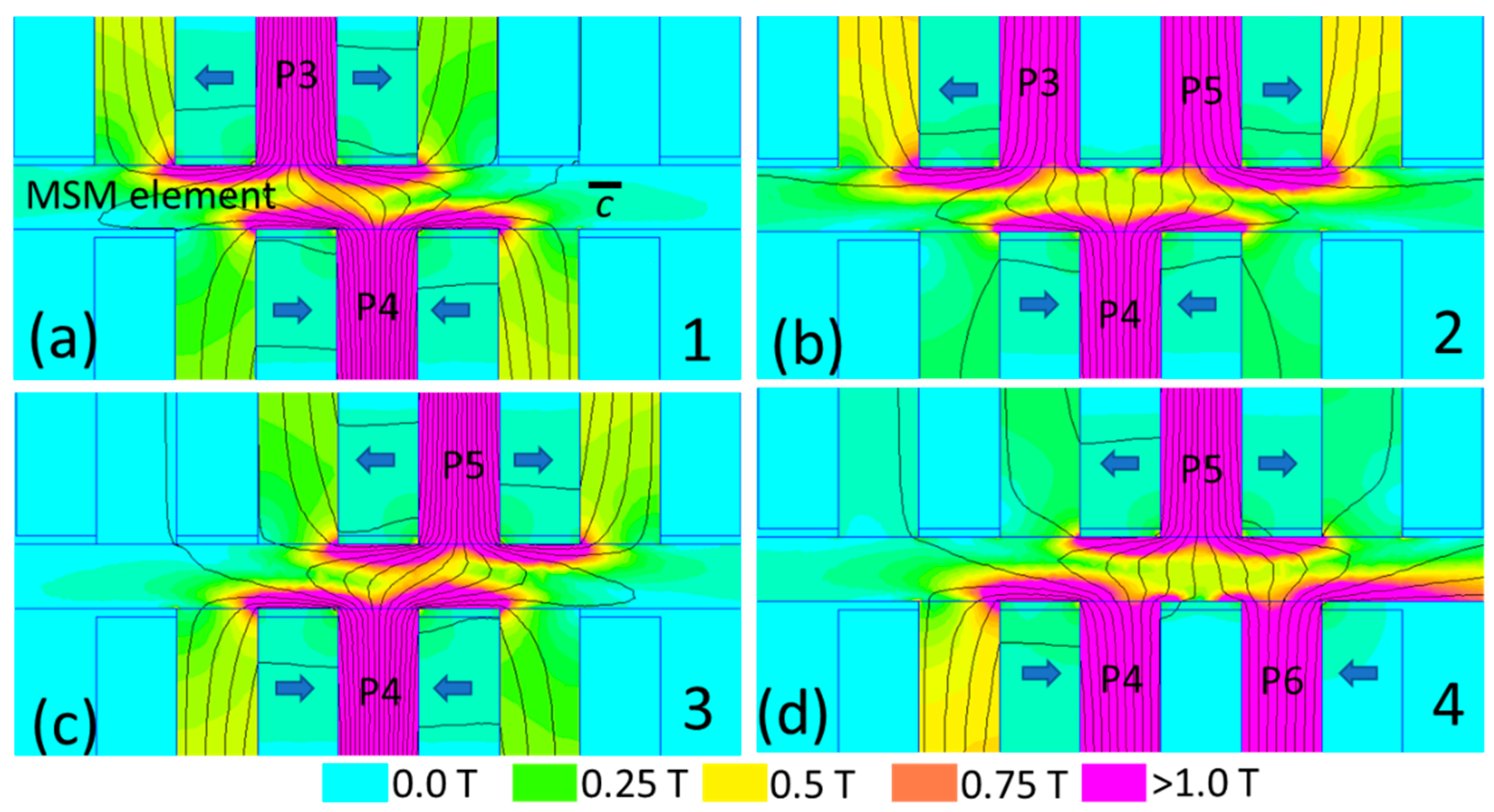
3.1. Simulated Cases

The magnetic field patterns were simulated first without any MSM element for the circuits described in Section 2.2. Then, the experimental and simulated values were compared to determine the validity of the FEMM simulations.

Second, the device was coupled to an MSM element that was fully compressed, with the c-axis oriented horizontally. Thus, the device magnetized the MSM sample along the hard magnetization axis. The pulse sequences 1–5 were simulated as described in Section 2.2. Thus, the simulations showed the magnetic field available to cause the switching effect in an unswitched element.

Then, the magnetic field with a twin in the element was modeled. The twin had c vertical and provided a path for the flux short through the MSM element. However, we were only guessing the position of the twin. The twin was moved to different locations, determining the magnetic flux pattern and interaction of the twin with the activated poles.

Finally, the magnetic field of a permanent magnetic drive was modeled. The simulations allow for comparison of the magnetic field energy between the permanent magnetic drive and the staggered pole electromagnet.

3.2. Magnetic Field Energy

FEMM was used to analyze the magnetic field energy in the drive (with and without the MSM element). The magnetic field energy of the permanent magnet is large and varies slightly with the configuration of the MSM element. The stray field interacts with the MSM element to lower the stray field energy. FEMM integrates the magnetic field energy (MFE) of the defined region as $W_m= {{\displaystyle \int }}_0^{B}HdB$ [20].

The MFE was evaluated for two areas. The region of interest (ROI) was the region of volume occupied by the MSM element. In some simulations, the drive was simulated without the MSM element, and the material within the ROI was air. The second area was the entire system. The total system energy was approximated within the system by evaluating a cylindrical volume with 60 mm diameter and zero-flux density boundary condition on the circumference. This cylindrical volume was centered on the drive system.

Then, the MFE in the MSM element for the staggered pole circuit was considered. A 2.0 mm thick twin was introduced to the element. For each pulse sequence (1–5), the twin was moved along the element, and the MFE of the MSM element was recorded at each position. The twin was moved in increments of 0.5 mm along the element. The total system and ROI MFE energies were evaluated to make direct comparison between the energetics of the electromagnetic drive and that of the permanent magnetic drive.

4. Results

4.1. Device Measurements

Figure 3 shows the experimental results of the flux generated in the air gap by the activation of circuit 1 (gray), circuit 2 (green), and circuit 3 (blue). The drive’s total current was recorded at each measurement and divided by the number of energized coils to determine the current per coil. The magnetization was quite similar for circuits 1, 2, and 3. The red curve shows the activation of only P4 by coils B2 and B3 alone. In the red curve, the magnetic induction began to saturate at a lower field in the airgap than for the other circuits, which have two energized poles.

No motion of twin boundaries was detected for the pulsing sequence. Before and after pulsing, the twin boundary geometries were identical. A slight motion appeared to be due to Maxwell forces at the poles that attracted the MSM element.

4.2. FEMM Simulation

The magnetic induction in the airgap was approximately 250 mT at 1 A on each coil, which correlated well to the experimental measurements of Figure 3.

Figure 4 shows the elementary sequence of circuits that advances the vertical flux along the single variant MSM element. In Figure 4a, circuit 1 activated poles P4 and P3. In Figure 4b, circuit 2 activated P4 and also P3 and P5. In Figure 4c, circuit 3 activated P4 and P5. In Figure 4d, circuit 4 activated P4 and P6 on the bottom yoke, and P5 on the top. The circuit number following Section 2.2 is noted in the bottom right of each frame in Figure 4.

When activated with circuit 1 (Figure 4a), poles P3 and P4 were saturated and directed magnetic flux between them. A significant portion of the flux generated by the individual poles leaked back through adjacent poles P2 and P6, rather than continuing to the other side of the MSM element. When activated with circuit 2 (Figure 4b), the vertical field in the MSM element was broad, and some flux lines circled back to adjacent poles. Activated with circuit 3 (Figure 4c), the field pattern was symmetrical to that of circuit 1. Pole 2 leaked slightly more induction than pole 3. Activated by circuit 4 (Figure 4d), the pattern was symmetrical to circuit 2, which was advanced by half a pole pitch.

Figure 5 shows the line profiles for the circuits that complete the switching pattern in the parent variant. The line position is shown in Figure 2 as the red horizontal line. The peak field takes either of two values. Circuits 1, 3, and 5 have narrower peaks and a lower peak maximum with about 0.3 T. Circuits 2 and 4 have broader peaks and a peak maximum of about 0.47 T. The broadening of the peaks is because three poles conduct the flux. The vertical field moves 6.0 mm from peak to peak, which gives the stroke of the elementary sequence.

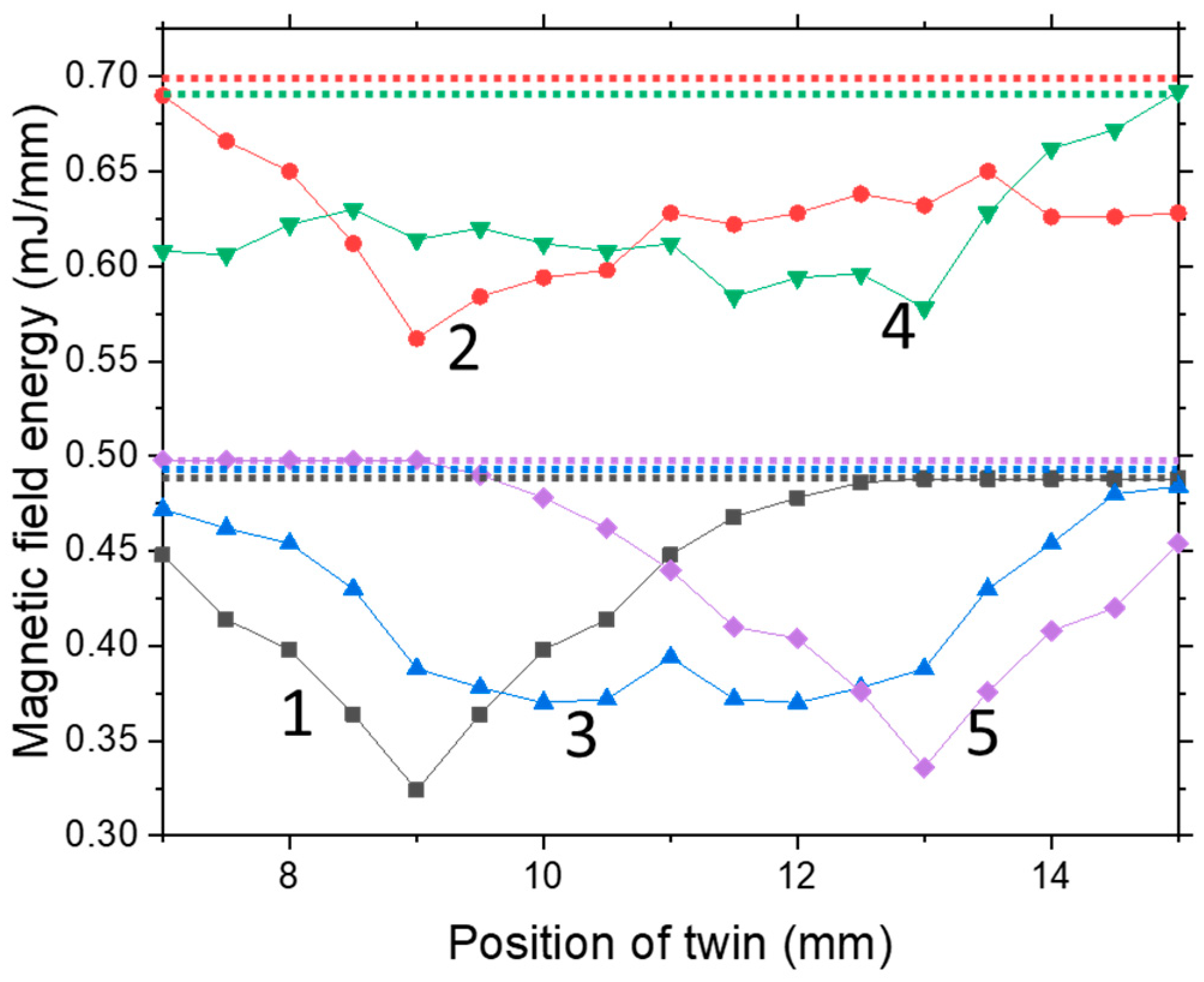
4.2.1. MSM Element with a Twin

The switching of the material had a large effect on induction [21]. Figure 6 shows the induction along the red line in air, the parent variant, and the parent variant with a twin, activated by circuit 1. In air, the peak of the flux was 251 mT. For the material unswitched in the parent variant, the peak maximum was 334 mT. When switched, i.e., with a twin in the MSM element, the field in the twin exceeds 1.4 T. The induction values for the twin were higher than the material’s magnetic saturation of about 600 mT [16].

Figure 7 shows simulation results with a twin at three different locations, namely between poles P3 and P4 (Figure 7a), between poles P4 and P5 (Figure 7b,c), and between poles P5 and P6 (Figure 7d). In the first situation, poles P3 and P4 were energized (i.e., circuit 1); in the other three cases, poles P4 and P5 were energized (i.e., circuit 3). In Figure 7a, the twin was evenly saturated across its width. The broad, symmetric peak of the twin in Figure 6 corresponds to the even saturation at the sample center, across the twin.

In Figure 7b, the magnetic flux entered the twin vertically; then, it was refracted across the twin boundary, to be horizontal in the element, before it exited the MSM element and entered P5. The right twin boundary was highly magnetized, while the left twin boundary was almost void of magnetic flux.

In Figure 7c, the flux narrowly constricted at a location defined by the connection of the right side of P4 and the left side of P5. With the advancement of the mechanism, in Figure 7d, the situation was the opposite of Figure 7b, with the left twin boundary redirecting substantial magnetic flux and the right boundary in a region of low induction. In a next step (not shown here), poles P5 and P6 were activated with the twin at the position as in Figure 7d. The resulting magnetic flux pattern was identical to that shown in Figure 7a but displaced by one pole pitch to the right.

Figure 8 shows profiles (a) through (d) corresponding to the simulation scenarios of Figure 7. For profile (e), the twin was in the position as in (d), but circuit 5 was energized. For this situation, the magnetic flux pattern was nearly identical to that of Figure 7a, though it was advanced by a pole pitch. The induction calculated by FEMM was higher than possible for the MSM sample, which has a saturation magnetization of about 600 mT [16]. The deviation was due to FEMM’s linear approximation of the anisotropic magnetic permeability.

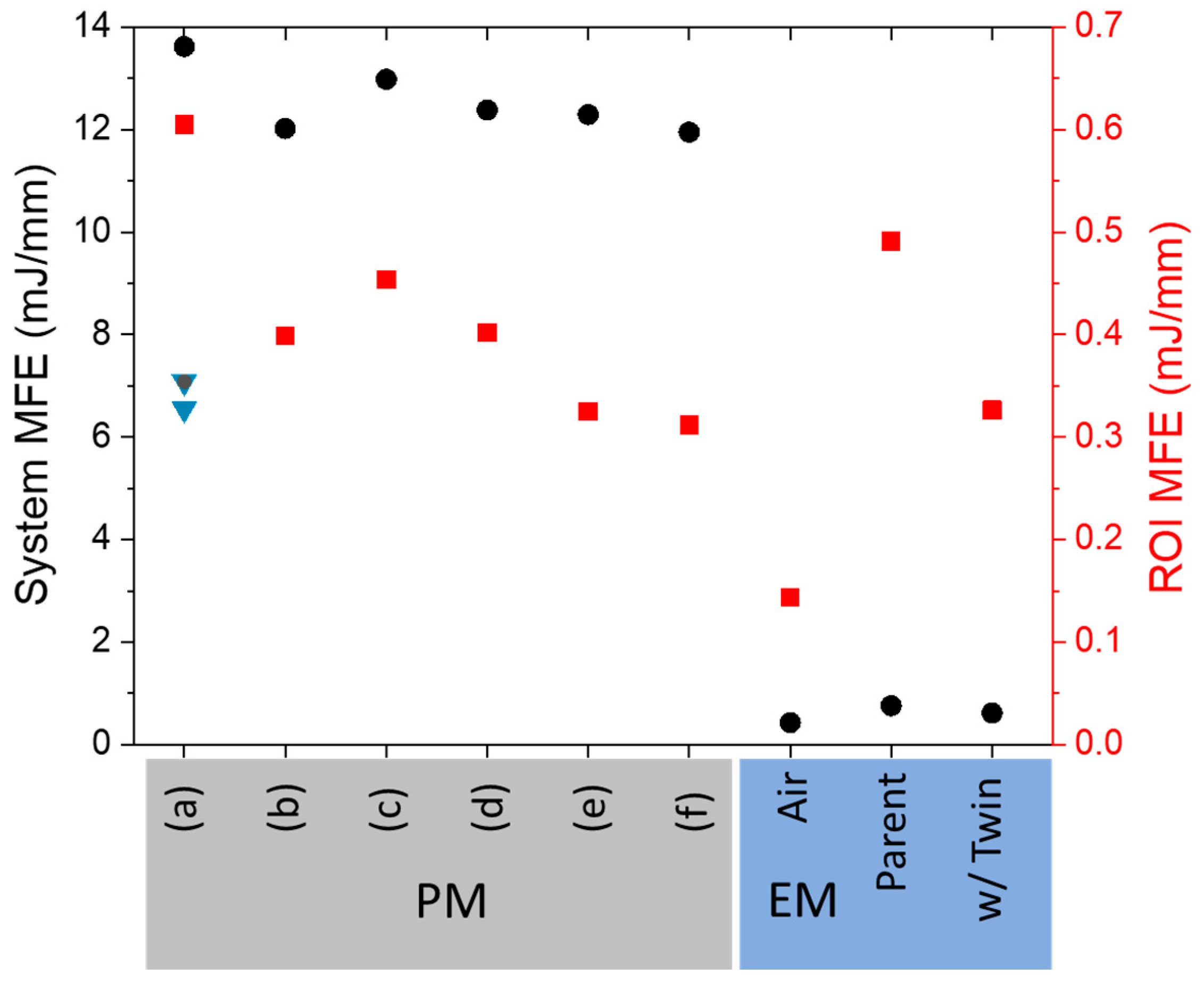
4.2.2. Simulation of Magnetic Field Energies (MFE)

Figure 9 shows the MFE for each magnetic circuit (1–5) as a function of twin positions. The units of MFE were recorded in mJ/mm, which gives the energy for each mm depth of our two-dimensional (planar) simulation. Initially, the MFE for the parent variant MSM element was recorded without any twin, which is represented in Figure 9 as dashed horizontal lines with the same color as the active circuit.

Circuits 2 and 4 had higher MFE than 1, 3, or 5. The deviation in energy between the single variant (dashed line) and the energy minima was the energy variation available to nucleate the twin. The energy reduction of circuit 2 compared to the single variant condition (dashed line) had a maximum of 0.12 mJ/mm at 9 mm. The local minima at 9 mm was distinct. The energy variation between adjacent positions was steep on the left side of the minima, yet shallow on the right side. The energy configurations for circuit 4 are nearly symmetrical to those of circuit 2.

Circuits 1, 3, and 5 had lower MFE for the single variant condition. The MFE for the three circuits was about 0.49 mJ/mm. The energy variation of circuit 1 was 0.155 mJ/mm, which is slightly greater than that of circuit 2. Circuit 1 had a clear and distinct energy minimum compared to circuit 2.

Circuit 3 had similar single variant MFE to circuits 1 and 5. The circuit does not have a distinct minimum, though. The profile takes two shallow troughs separated by a slight peak, which arose at the connection of the troughs. This behavior is interpreted as the twin being relatively stable from about 9 to 13 mm, but with little preference for position.

Figure 10 shows results of simulation of the permanent magnetic drive (PM). In Figure 10a, the magnet was surrounded by air. The system energy was found within the 60 mm boundary condition. The element energy was found within the dashed black box indicated in Figure 10a. Figure 10b shows simulation now with a parent region in the dashed box. The magnetic stray field, which previously entered the air-gap in Figure 10a, was directed horizontally to the ends of the parent variant and back down to the permanent magnet. In Figure 10c, the region was a single variant, which has the c axis oriented vertically (i.e., perpendicular to the axis of the MSM element). The magnetic anisotropy directed magnetic flux up, causing a large magnetic stray field, similar to the magnetic flux distribution in the airgap. In Figure 10d, a twin was introduced, which split the element in half. The parent variant (with c horizontal) was on the left and the twin (with c vertical) was on the right. Flux concentrates in the parent variant and only weakly magnetizes the twin. In Figure 10e, the situation was reversed. Here, the twin magnetized strongly underneath the twin boundary, and in the parent variant, it refracted across the twin boundary. In Figure 10f, a twin was created between two parent variants. Similarly, to Figure 10e, magnetic flux concentrated underneath the twin boundary. The parent variant on the left directed flux horizontally. A minimal stray field was present above the element in Figure 10b,c.

Figure 11 shows a comparison of the magnetic energies of the permanent magnetic drive and the staggered pole electromagnetic (EM) drive. The horizontal axis indicates the simulation. (a) gives the energies corresponding to Figure 10a. The black circle is the system energy. The upside-down triangles show the magnetic field energy in the magnet (gray) and the stray field (blue). The red square indicates the magnetic field energy in the boxed region, which in this simulation was air. The red squares are read by the right axis, which shows finer energy variations. Thus, for (a), the system energy was 13.62 mJ/mm, the MFE in the permanent magnet was 7.08 mJ/mm, and the MFE for the stray field was 6.54 mJ/mm. The MFE in the ROI was 0.61 mJ/mm. In (b), the air region was changed to the parent variant, and the MFE for the system and ROI were defined. The system and ROI energy are decreases relative to (a). In (c), the parent variant was changed to the twin variant, and it shows switching of the entire element. The system and ROI energy were greater than for the parent variant but less than for the air. In (c,d), a twin boundary split the volume of the ROI equally into twin and parent. With the parent on the right (d), the system energy is in-between that of the single variant parent or twin. The ROI energy is about the same as for the parent. With the parent on the left, the system energy was slightly decreased, and the ROI energy decreased more substantially. In (e), with a single thick twin in the center of two parent variants, the system energy and the ROI energy are the lowest for the permanent magnetic drive.

Figure 11 shows the MFE for three simulations of the electromagnetic (EM) drive for the activation of circuit 1. With an airgap separating the top and bottom yokes, the total system MFE was 0.43 mJ/mm. The MFE in the airgap region was 0.14 mJ/mm. With a parent variant MSM element inserted, the system’s MFE energy increased to 0.75 mJ/mm. The MFE of the MSM element was 0.49 mJ/mm. With a twin connecting poles P4 and P3, as in Figure 7a, the systems energy was slightly lower, and the energy of the MSM element decreased compared to the parent variant, at 0.33 mJ/mm. The system MFE of the electromagnetic drive was almost an order of magnitude less than that for the permanent magnetic drive.

5. Discussion

There is a significant difference between the actuator properties of the permanent magnetic drive and the electromagnetic drive. The permanent magnetic drive creates a twin in the material and then translates the twin along the MSM element [8]. The electromagnetic drive does not readily generate the twin nor move the twin boundaries. For the permanent magnetic drive, the vertical magnetic field that first caused deformation was about 200 mT [8]. The electromagnetic drive here generates a 300 mT magnetic field in the airgap. Our previous device in [10] required a field measured in the airgap of 500 mT to nucleate a twin, which is more than three times more than the switching field of 150 mT measured along the short direction in a vibrating sample magnetometer. Thus, the local magnetic switching field is perhaps three times the global magnetic switching field.

The MFE was calculated using FEMM. The method disregards the contributions of the Zeeman energy and lowering of anisotropy energy by variant reorientation. The anisotropy energy was found in Section 3.2 to be about 0.6 mJ for a 3.0 mm³ twin band, which is small for the permanent magnet yet significant for the EM drives. Significant sections of our element exhibit magnetic saturation, which causes additional significant error to the MFE.

In Figure 11a, the energy of the permanent magnet and the stray field without an MSM element is 13.6 mJ/mm. The permanent magnet in a PM drive is 12.7 mm long. The multiplication of these two numbers gives an MFE of 172 mJ for the system. The minimum required length of the magnet is unknown; however, if it was only as wide as the element (2.0 mm), the MFE would be 27.2 mJ. The energy needed to cause a shrinkage to form and move through the element has been experimentally measured by Smith et al. as 0.77 mJ by the difference in energy of a motor before and after coupling to the MSM element [9]. In Figure 11, by taking either the parent single variant or the twin within the parents, the stray field is reduced by about 1 mJ per mm depth of simulation. Thus, for a 2.0 mm wide MSM element, the energy reduction would be 2.0 mJ. This is perhaps not the only energy given to the MSM element, which can draw also 0.6 mJ of anisotropy energy.

For the EM drive, the MSM element can draw energy proportional to its reluctance. The maximum system energy is 0.76 mJ/mm depth, which translates for our physical device, which has a yoke depth of only 3 mm, to a maximum output of 2.28 mJ.

The variation of the stray field energy for just the MSM element is actually greater in the electromagnetic drive. A permanent magnet acts as a constant source of magnetic flux, analogous to a current source in electronics. In contrast, the electromagnetic coils act as a generators of flux potential, analogous to a voltage driving a current according to the circuit’s resistance. The flux induced by the coils is a function of the reluctance of the circuit. When the reluctance is decreased, e.g., by insertion of the MSM element, the magnetic flux across the entire system increases. The different behaviors can be seen in Figure 11. When the MSM element is added to the magnetic circuit of the permanent magnetic drive, the total system energy decreases. The electromagnetic drive initially has a low system energy, as the airgap causes a large reluctance gap and reduces generated flux in the system. When the MSM element is inserted, the system energy increases by 79%.

Our device has a relatively high physical pole density. However, this does not necessarily translate to the creation of a high density of stable twin positions. In Figure 9, only circuits 1 and 5 have distinct energy minima. Circuits 2 and 4 have low energy variations, and the energy minima are at the same position as for circuits 1 and 5 (i.e., no motion of the minima). Circuit 3 exhibits a shallow depression, which is composed of two shallow troughs. The slight peak between the troughs indicates that a twin at this position is a bit unstable. The local minima observed do not account for the anisotropy energy, which together with the Zeeman energies affects the total system energy configuration, which drives the deformation. However, the calculation of all energies is quite challenging.

The energies of a single domain MSM element in the field of a permanent magnetic (Figure 10b) and the energy of an MSM element with a small twin (Figure 10f) are almost identical. The creation of the twin reduces the magnetic stray field energy by only 0.07 mJ/mm while decreasing anisotropy nearly 0.6 mJ. This indicates that other energy contributions play a significant role, such as the magnetocrystalline anisotropy energy. Further analysis of this situation is required, which is beyond the scope of this study.

6. Conclusions

An MSM element was exposed to localized magnetic fields in two ways: (1) with a permanent magnet, (2) with sets of electrical coils and yokes. The magnetic field strength at the position of the MSM element was similar for the two cases and larger than the magnetic switching field. For the permanent magnet, the magnetic field nucleated twins, while it was not so for the electromagnetic drive. This variation is attributed (1) to the high energy carried in the stray field of the permanent magnet, and (2) to the coils generating a magnetic flux potential where the actual magnetic flux depends on the reluctance of the magnetic circuit. More detailed studies are required to develop a quantitative understanding of the localized switching of MSM elements in heterogeneous magnetic fields.

References

1. Costanza, G.; Stefano, P.; Maria, E.T. IR Thermography and Resistivity Investigations on Ni-Ti Shape Memory Alloy. Key Eng. Mater. 2014, 605, 23–26. [Google Scholar] [CrossRef]
2. Lin, Y.C.; Lin, C.F. Microstructures and magnetic properties of Fe–Ga and Fe–Ga–V ferromagnetic shape memory alloys. IEEE Trans. Magn. 2015, 51, 1–4. [Google Scholar] [CrossRef]
3. Kuchin, D.; Elvina, D.; Yurii, K.k.; Alexander, K.; Victor, K.; Alexey, M.; Vladimir, S.; Jacek, C.; Krzysztof, R.; Vladimir, K. Direct measurement of shape memory effect for Ni54Mn21Ga25, Ni50Mn41. 2In8. 8 Heusler alloys in high magnetic field. J. Magn. Magn. Mater. 2019, 482, 317–322. [Google Scholar] [CrossRef]
4. Suorsa, I.; Tellinen, J.; Ullakko, K.; Pagounis, E. Voltage generation induced by mechanical straining in magnetic shape memory materials. J. Appl. Phys. 2004, 95, 8054–8058. [Google Scholar] [CrossRef] [Green Version]
5. Lindquist, P.; Hobza, T.; Patrick, C.; Müllner, P. Efficiency of Energy Harvesting in Ni–Mn–Ga Shape Memory Alloys. Shape Mem. Superelasticity 2018, 4, 93–101. [Google Scholar] [CrossRef]
6. Karaman, I.; Basaran, B.; Karaca, H.E.; Karsilayan, A.I.; Chumlyakov, Y.I. Energy harvesting using martensite variant reorientation mechanism in a NiMnGa magnetic shape memory alloy. Appl. Phys. Lett. 2007, 90. [Google Scholar] [CrossRef]
7. Ullakko, K.; Wendell, L.; Smith, A.; Mullner, P.; Hampikian, G. A magnetic shape memory micropump: Contact-free, and compatible with PCR and human DNA profiling. Smart Mater. Struct. 2012, 21. [Google Scholar] [CrossRef]
8. Saren, A.; Smith, A.R.; Ullakko, K. Integratable magnetic shape memory micropump for high-pressure, precision microfluidic applications. Microfluid. Nanofluid. 2018, 22. [Google Scholar] [CrossRef]
9. Smith, A.R.; Saren, A.; Jarvinen, J.; Ullakko, K. Characterization of a high-resolution solid-state micropump that can be integrated into microfluidic systems. Microfluid. Nanofluid. 2015, 18, 1255–1263. [Google Scholar] [CrossRef]
10. Ullakko, K. Magnetically controlled shape memory alloys: A new class of actuator materials. J. Mater. Eng. Perform. 1996, 5, 405–409. [Google Scholar] [CrossRef]
11. Armstrong, A.; Karki, B.; Smith, A.; Müllner, P. Traveling Surface Undulation on a Ni-Mn-Ga Single Crystal Element. Submitted for Publication. Available online: https://core.ac.uk/download/pdf/334778582.pdf#page=127 (accessed on 23 February 2021).
12. Smith, A.; Tellinen, J.; Mullner, P.; Ullakko, K. Controlling twin variant configuration in a constrained Ni-Mn-Ga sample using local magnetic fields. Scr. Mater. 2014, 77, 68–70. [Google Scholar] [CrossRef]
13. Armstrong, A.; Finn, K.; Hobza, A.; Lindquist, P.; Rafla, N.; Mullner, P. A motionless actuation system for magnetic shape memory devices. Smart Mater. Struct. 2017, 26. [Google Scholar] [CrossRef] [Green Version]
14. Jiles, D. Introduction to Magnetism and Magnetic Materials; CRC Press: Boca Raton, FL, USA, 2015. [Google Scholar]
15. Kellis, D.; Smith, A.; Ullakko, K.; Mullner, P. Oriented single crystals of Ni-Mn-Ga with very low switching field. J. Cryst. Growth 2012, 359, 64–68. [Google Scholar] [CrossRef]
16. Schiepp, T.; Maier, M.; Pagounis, E.; Schluter, A.; Laufenberg, M. FEM-Simulation of Magnetic Shape Memory Actuators. IEEE Trans. Magn. 2014, 50. [Google Scholar] [CrossRef]
17. Gómez, E.; Roger-Folch, J.; Molina, A.; Fuentes, J.A.; Gabaldón, A.; Torres, R. Modelling of magnetic anisotropy in the finite element method. COMPEL 2006, 25, 609–615. [Google Scholar] [CrossRef]
18. Heczko, O.; Straka, L.; Lanska, N.; Ullakko, K.; Enkovaara, J. Temperature dependence of magnetic anisotropy in Ni-Mn-Ga alloys exhibiting giant field-induced strain. J. Appl. Phys. 2002, 91, 8228–8230. [Google Scholar] [CrossRef] [Green Version]
19. Suorsa, I.; Pagounis, E.; Ullakko, K. Position dependent inductance based on magnetic shape memory materials. Sens. Actuators a-Phys. 2005, 121, 136–141. [Google Scholar] [CrossRef]
20. Meeker, D. Finite Element Method Magnetics—Version 4.0 User’s Manual; University of Virginia: Charlottesville, VA, USA, 2006. [Google Scholar]
21. Suorsa, I.; Pagounis, E.; Ullakko, K. Magnetization dependence on strain in the Ni-Mn-Ga magnetic shape memory material. Appl. Phys. Lett. 2004, 84, 4658–4660. [Google Scholar] [CrossRef] [Green Version]
Figure 1. Design of the electromagnetic drive: (a) finite element method magnetics (FEMM) simulation including the Fe-Co yoke geometry, pole geometry, and coil geometry. The bottom yoke contains the bottom poles P2, P4, and P6 and slides between the tines of the top yoke. The bottom and top yokes had poles that were staggered relative to each other. (b) shows the machined device before winding the outermost coils.
Metals 11 00536 g001
Figure 2. Schematic of the poles (P1–P7), the bottom yoke poles (B1–B4), and the top yoke coils (T1–T5). The flux density was measured in the center of the air gap, at location H1, for sequence 1. The hall probe (the red box) recorded data at positions H2 and H3 for the pulsing sequences measured experimentally.
Metals 11 00536 g002
Figure 3. Experimental data of the magnetic induction in the air gap as a function of the applied current. In gray (squares), the results of pulse sequence 1, measured at Hall sensor location H1. In green (triangles pointing down), the energized sequence 2 measured at H2. The blue pulse sequence 3 (triangles pointing up), measured at H3. The red data (circles) shows activation of just the P4 pole by coils B2 and B3, at H2.
Metals 11 00536 g003
Figure 4. FEMM simulation of the pulsing sequence which approximates a moving vertical field. The simulation shows the fields induced in a single variant MSM element with the c-axis oriented horizontally. (a) shows circuit 1, which sent flux up and left. In (b) circuit 2 caused vertical and symmetrical flux. (c) shows circuit 3, which had identical flux to circuit 1, but mirrored in the vertical to be up and right. In (d), Circuit 4 had flux identical to that of circuit 2, but mirrored across horizontal and advanced a pole pitch.
Metals 11 00536 g004
Figure 5. Profiles of the induction of the single variant element for circuits 1–5.
Metals 11 00536 g005
Figure 6. The twin has induction much greater than that for the parent variant, or air. The profiles show the profile along the center of the simulations presented in Figure 2, Figure 4a and Figure 7a.
Metals 11 00536 g006
Figure 7. FEMM simulations of circuit 1 for (a) and circuit 3 for (bd). The location of the twin affected the magnetic flux pattern. In (a), a twin variant was between P3 and P4 using circuit 1. In (b), with circuit 3 activated, the field interacts with the twin still at the location of (a). Then, the twin was moved further along the element in (c,d). In (c), the magnetic flux was locally concentrated in a strong vertical magnetic field. In (d), the magnetic flux reflected strongly across the left twin boundary, in a pattern symmetrical to that of (b).
Metals 11 00536 g007
Figure 8. Simulation of the flux density along the magnetic shape memory (MSM) element, including a twin region. The twin region moved along the element corresponding to the (ad) sequences in Figure 7. (e) profile shows the simulation of the (d) twin boundary position, using circuit 5.
Metals 11 00536 g008
Figure 9. Drive energy at configurations of a 2.0 mm wide twin moving through the studied circuits (1–5). The dotted lines correspond to the circuit by color and give the energy of the single variant condition.
Metals 11 00536 g009
Figure 10. FEMM simulation of the magnetic flux pattern of the permanent magnetic drive. In (a), the cylindrical magnet generated a magnetic dipole field in air. In (b), the boxed region was defined as the parent variant with the c-axis oriented horizontally. (c) shows the boxed region defined as a single variant of twin with the c axis oriented vertically. In (d), a twin boundary in the center separated the twin and parent into equal volumes. The left volume was defined as the parent (c horizontal), and the right was defined as the twin (c vertical). In (e), a twin boundary again separates equal twin volumes; however, the twin was defined on the left and the parent was defined on the right. In (f), two twin boundaries were inserted with a twin in between, at the center of the parent variant. The energy within the dashed box is highest in air and lowest with two twin boundaries.
Metals 11 00536 g010
Figure 11. Comparison of the magnetic field energies for the Figure 10 configurations of the permanent magnetic (PM) to configurations of the electromagnetic (EM) drive. The black circles show the magnetic field energy of the entire system read on the left axis. Red squares show the magnetic field energy of the ROI region and reads according to the right axis. The triangles show the magnetic field energy in the magnet (black triangle) and in the magnets stray field (blue triangle) for simulation of the permanent magnet in air. (a) shows the energies for the permanent magnet drive in air, the magnet with single variant parent configuration (b) and single variant twin configuration (c). (d) with a twin boundary in the center separating parent and twin variants on the right and left, and (e) with the variants switched in position. (f) shows the magnetic field energy associated with a band of twin variant between two parent variants.
Metals 11 00536 g011
Publisher’s Note: MDPI stays neutral with regard to jurisdictional claims in published maps and institutional affiliations.