Flow Stress of 6061 Aluminum Alloy at Typical Temperatures during Friction Stir Welding Based on Hot Compression Tests

Abstract

The purpose of this paper is to report quantitative data and models for the flow stress for the computer simulation of friction stir welding (FSW). In this paper, the flow stresses of the commercial 6061 aluminum alloy at the typical temperatures in FSW are investigated quantitatively by using hot compression tests. The typical temperatures during FSW are determined by reviewing the literature data. The measured data of flow stress, strain rate and temperature during hot compression tests are fitted to a Sellars–Tegart equation. An artificial neural network is trained to implement an accurate model for predicting the flow stress as a function of temperature and strain rate. Two models, i.e., the Sellars–Tegart equation and artificial neural network, for predicting the flow stress are compared. It is found that the root-mean-squared error (RMSE) between the measured and the predicted values are found to be 3.43 MPa for the model based on the Sellars–Tegart equation and 1.68 MPa for the model based on an artificial neural network. It is indicated that the artificial neural network has better flexibility than the Sellars–Tegart equation in predicting the flow stress at typical temperatures during FSW.

1. Introduction

Friction stir welding (FSW) [1,2,3,4,5,6] is an advanced solid-state welding technology for joining structural metals, such as aluminum alloys [7] and magnesium alloys [8]. In FSW, a rigid rotating tool plunges into the workpieces and travels along the interface to be joined. The friction between the rotating tool and the workpiece leads to significant heat generation. As a result, the metals in the vicinity of the welding tool are heated and softened. The friction-induced plastic flow occurs in the vicinity of the welding tool, which results in sound solid-state bonding at the interface [9]. The in-process plastic flow during FSW is very important in understanding the generation [10], heat transfer [11], microstructure evolution [12,13] and defect formation [14,15]. Flow stress at the welding temperature, which determines the viscosity, is one of the physical factors that govern the momentum transfer and mass transfer in plastic flow during FSW. Due to the complexity of the problem, computer simulation [16,17] has been the major approach for investigating the in-process plastic flow pattern during FSW. Because of the critical role that the material flow plays, reliable quantitative models for predicting the flow stress at high temperatures are generally desired as a part of the material model in the simulation of FSW processes.

In the previous computer simulations for FSW, models for predicting the flow stress of metals in other hot working processes, such as extrusion and rolling, have been applied in the simulation model for FSW. As both temperature and strain rate changes sharply in the vicinity of the welding tool during FSW, flow stress is necessary to consider as a function of both temperature and strain rate. The equation proposed by Sellars and Tegart [18] is one of the most widely used methods for predicting the flow stress at high-temperature as a function of both temperature and strain rate. In the early simulations, Collegrove et al. [19] employed the Sellars–Tegart equation to represent the flow stress of 5083 aluminum alloy in their simulation model based on computational fluid dynamics (CFD). Nandan et al. [11] adopted the Sellars–Tegart equation to calculate the flow stress of mild steel in their CFD analysis of the temperature and material flow during FSW. In a recent smoothed particle hydrodynamics model for FSW, Pan et al. [20] applied the Sellars–Tegart equation in predicting the flow stress of AZ31 magnesium alloy. Researchers have also extended the Sellars–Tegart equation in the simulation model for FSW regarding the uniqueness of the thermal conditions in FSW. It has been demonstrated that the temperature could be very close to the solidus temperature [21,22,23,24]; however, the Sellars–Tegart equation has been mostly applied in the typical temperature range of conventional hot working processes [25,26,27,28]. In other words, the typical temperatures during the conventional hot working processes are different from those during FSW. Currently, the quantitative data and models for the flow stress of metals at the typical temperatures in FSW are still insufficient. To develop simulation models for FSW, researchers have been looking for proper approaches for predicting the flow stress of metals at the typical welding temperatures. Colegrove et al. [29,30] proposed a linear empirical softening rule to calculate the flow stress of aluminum alloys when the temperature is close to the solidus temperature in the analysis of the heat generation and material flow of FSW processes. Due to the limitation in the temperature range of the Sellars–Tegart equation, other nonlinear terms [31,32,33] were adopted to calculate the flow stress when the temperature is close to the solidus temperature. However, the current methods for predicting the flow stress at the typical FSW temperature were empirical. Few experimental data on the flow stress when the temperature is close to the solidus temperature are available. Moreover, whether the Sellars–Tegart equation is feasible in representing the flow stress at typical FSW temperatures is also unknown.

In addition to the Sellars and Tegart equation, direct interpolation has been another method for calculating the flow stress at typical temperatures in FSW. In Chen et al.’s models [34,35] for FSW, a smooth function represents the temperature dependency of the flow stress. However, there has not been a generalized analytical function representing both the temperature dependency and the strain rate dependency of the flow stress. It has been recently demonstrated that the artificial neural network (ANN) [36,37,38,39,40] was successfully applied in the prediction of the flow stress, which depends on temperature, strain rate and strain because the ANN-based regression methods can fit complex mathematical relationships [41]. Although the feasibility of applying the ANN in modeling the flow stress is demonstrated, a comparative study is still needed to clarify the difference between the ANN method and the conventional method to support selecting a flow stress model in a simulation for FSW.

The purpose of this paper to report quantitative data and models for the flow stress for the computer simulation of friction stir welding (FSW). In this paper, models and data for predicting the flow stress of a commercial aluminum alloy 6061 (AA6061) at the typical temperatures during FSW are presented and studied. Quantitative data on the stress–strain curves were obtained by using hot compression tests. Both the Sellars–Tegart equation and the ANN are employed to establish a model for predicting the flow stress at typical temperatures during FSW. In addition, the Sellars–Tegart equation and ANN are discussed regarding their performance in predicting flow stress.

2. Materials and Methods

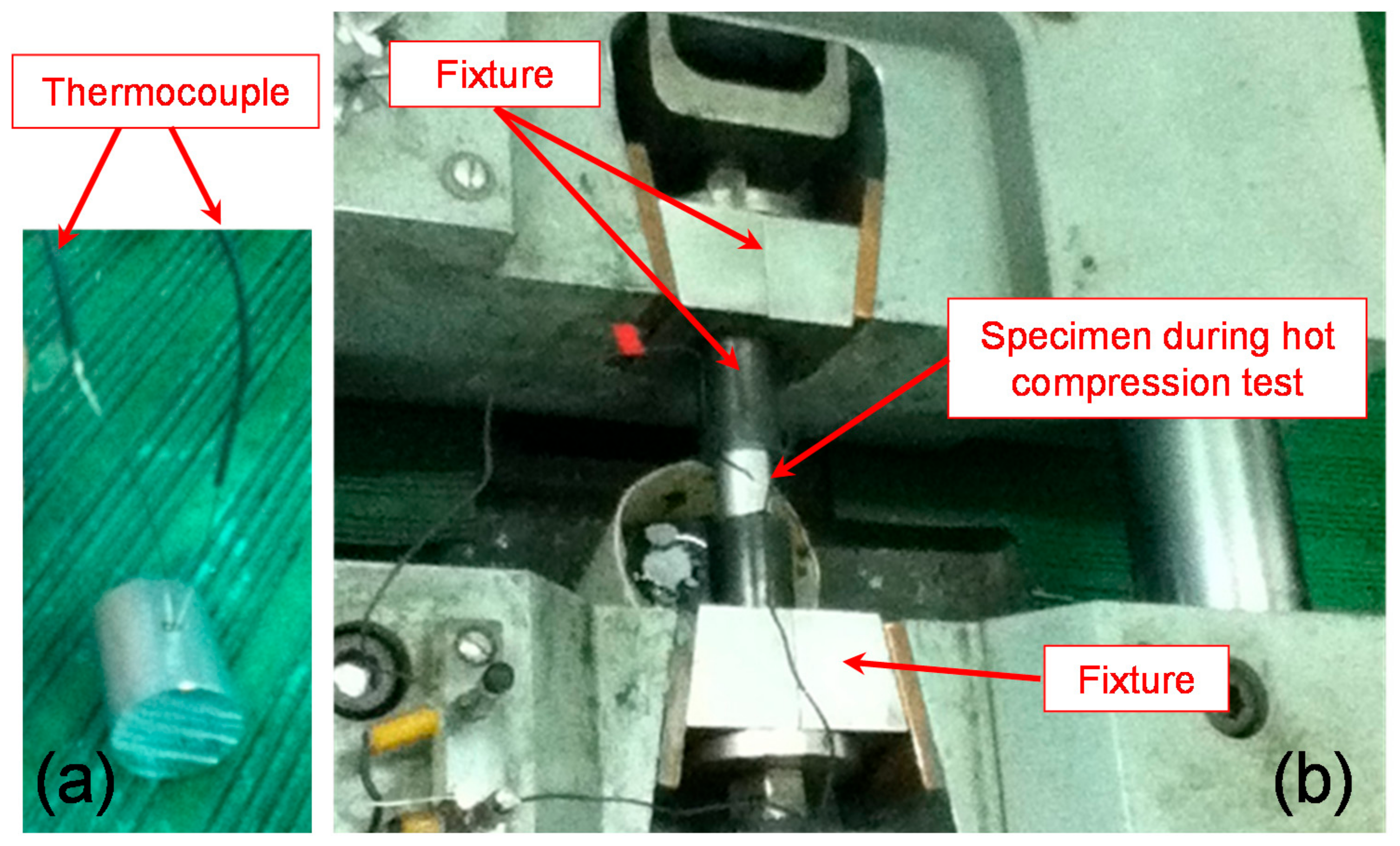
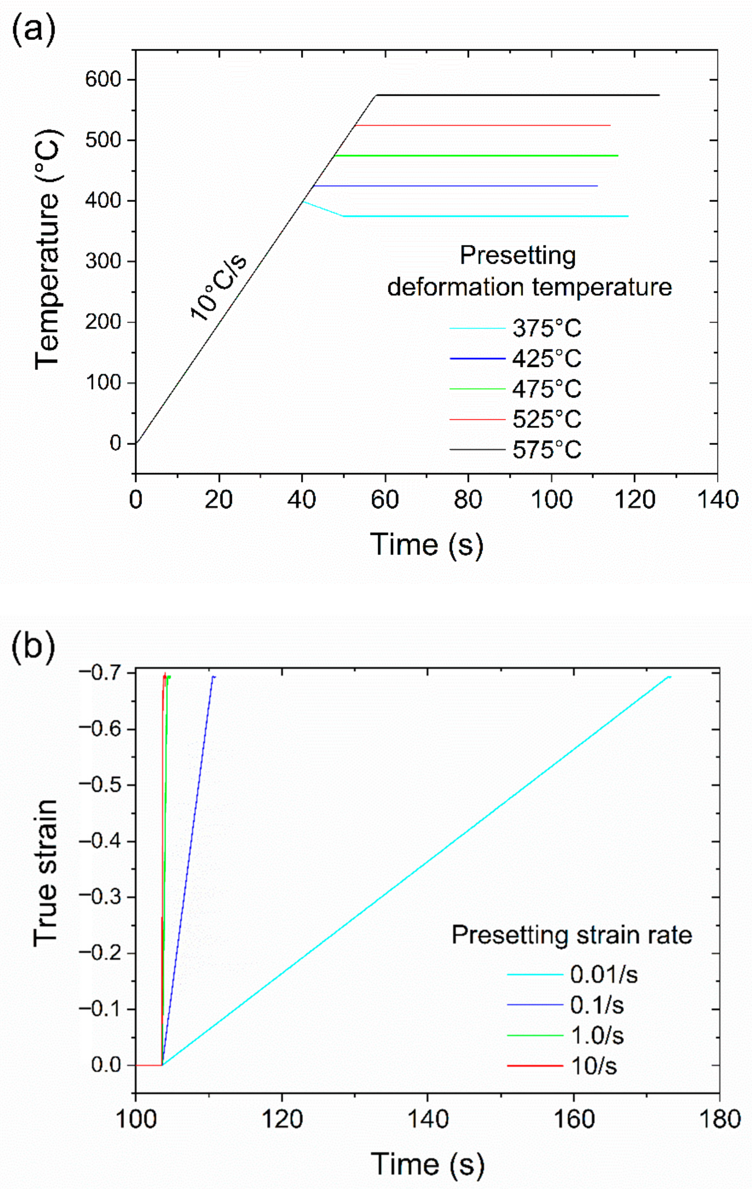
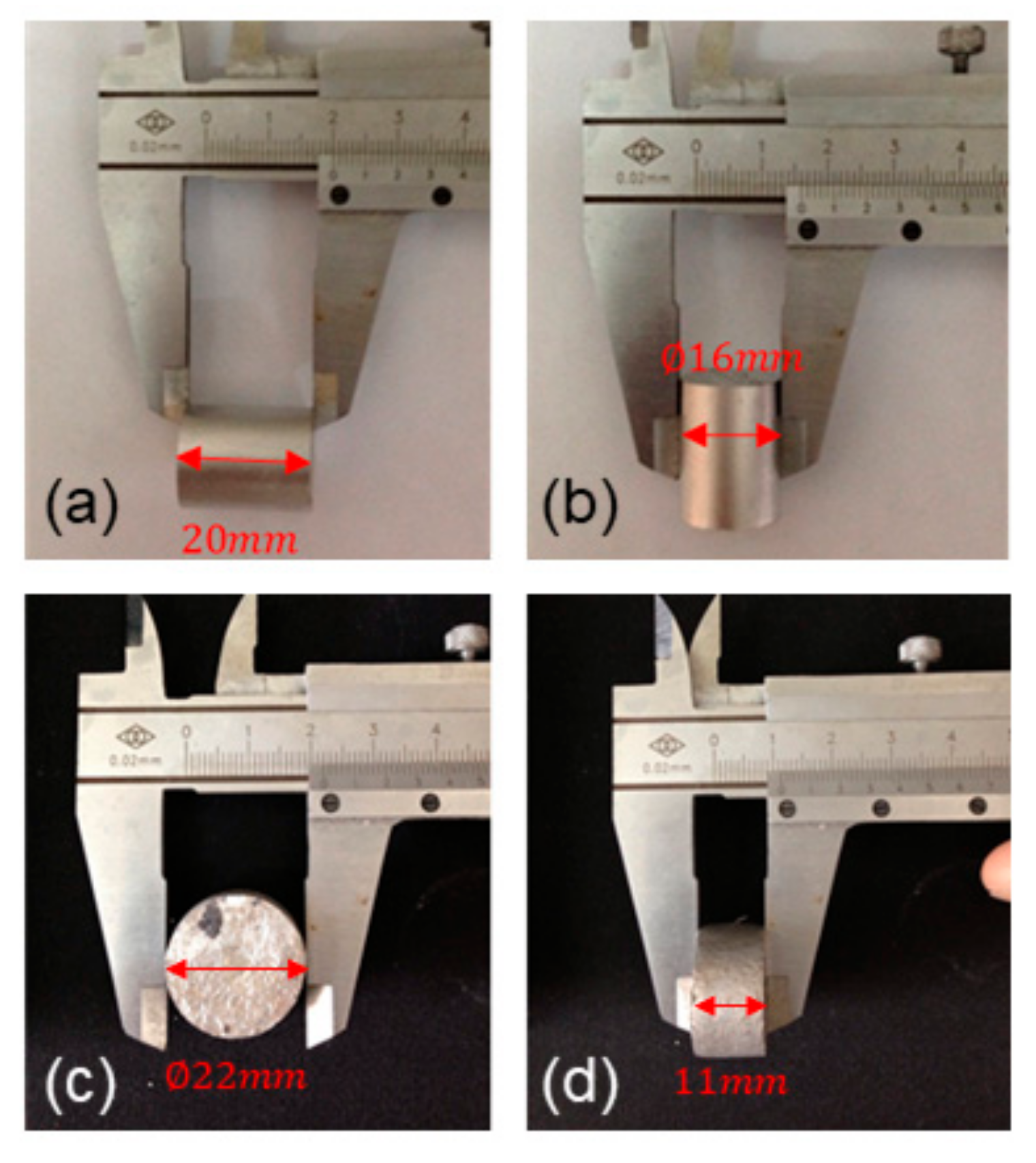
2.1. Hot Compression Tests

In this study, the commercial AA6061-T6 rod was used for testing flow stress. The chemical composition of AA6061 is shown in

Table 1. Chemical composition of commercial aluminum 6061 (mass fraction,%).

Element	Mg	Si	Cu	Cr	Fe	Mn	Zn	Ti	Al
Mass fraction, %	0.8~1.2	0.4~0.8	0.15~0.40	0.04–0.35	≤0.7	≤0.15	≤0.25	≤0.15	bal

. The uniaxial hot compression tests were conducted using a Gleeble-1500D system (Dynamic Systems Inc., Poestenkill, New York, USA). Before the tests, the prepared cylindrical specimens were 16 mm in diameter and 20 mm in height. As shown in Figure 1a, a K-type thermocouple is connected to the surface of the specimen for measuring the temperature. The reported temperature in the vicinity of the welding tool is shown in

Table 2. Typical in-process temperature during friction stir welding (FSW) of AA6061.

No.	Typical Temperature in FSW	Reference
1	383 °C~408 °C	[42]
2	487 °C~547 °C	[43]
3	477 °C~571 °C	[44]
4	413 °C~456 °C	[45]
5	427 °C~477 °C	[46]
6	518 °C~536 °C	[47]
7	541 °C	[48]

. It can be found that the reported temperature in FSW ranges from 383 °C to 571 °C. To conduct hot compression tests at typical temperatures during FSW, the testing temperatures in the uniaxial hot compression tests were designed to be 375 °C to 575 °C with an interval of 50 °C. The configuration of the hot compression tests is shown in Figure 1b. The designed thermomechanical history is shown in Figure 2. During the hot compression, the specimen was heated up to the target deformation temperature, as shown in Figure 2a. When the target deformation temperature was 375 °C, the sample was heated up to 400 °C at the rate of 10 °C/s and then cooled to 375 °C. When the target deformation temperature was 425 °C, 475 °C, 525 °C or 575 °C, the specimen was heated up to the target deformation temperature directly at the rate of 10 °C/s. Thereafter, the temperature was held at the targeted deformation temperature for 60 s. The hot compression test was carried out with the target strain rate after the temperature holding. The compressive true strain rate was taken as 0.01 /s, 0.1 /s, 1 /s, and 10 /s, respectively. Figure 2b shows the strain histories when the target deformation temperature was 425 °C as an example, and the deformation started at ~103 s. Figure 3 shows the geometry of the sample before and after the hot compression. It could be seen that the samples were well kept in the cylinder geometry. Therefore, in this study, the calculation of the true stress–strain curve is based on the assumption of uniform deformation. After the hot compression tests, the specimen was cooled to room temperature. In the hot compression tests, the stress–strain curve and the temperature curve were recorded.

2.2. Preparation of Dataset for Building the Flow Stress Models

Predictive models for the flow stress are of critical importance for developing a computer simulation for FSW. In FSW, significant plastic flow occurs near the welding tool. It was known from Liu et al. [49]’s study that the typical value of the typical strain in the vicinity of the welding tool is ~30. In other words, the material that directly interacts with the tool during FSW is severely deformed. As such, the flow stress for large strains from 0.2 to 0.6 with an interval of 0.1 was used to build the dataset for the flow stress. Each data point in the data set includes the temperature, the strain rate and the flow stress. The measured temperature, rather than the presetting temperature, was used as the temperature variable for each data point in the data set. Therefore, there are a total of 100 data points in the dataset. Based on the dataset used in this research, two models, i.e., the Sellars–Tegart equation and artificial neural network, for predicting the flow stress are built in this paper.

2.3. Approaches for Determining the Constants in the Sellars–Tegart Equation

The Sellars–Tegart equation [18] is widely used to predict the flow stress as a function of the temperature and the strain rate. The Sellars–Tegart equation was formulated as [18]:

$$\dot{\mathsf{\epsilon }}\exp (\mathrm{Q}/\mathrm{RT})=\mathrm{A}{\left[\sinh (\mathsf{\alpha }\mathsf{\sigma })\right]}^{\mathrm{n}}$$

(1)

where ${\dot{\mathsf{\epsilon }}}_{\mathrm{n}}$ is strain rate, σ is flow stress, Q is a material constant, which is the deformation activation energy, R is gas constant (8.314 J/mol/K), T is the temperature in K and α, A, and n is material constants. In total, the constants Q, α, A, and n are needed to be calculated. To fit the constants, we rewrite equations (1) as:

$$\ln \dot{\mathsf{\epsilon }}+\mathrm{Q}/\mathrm{RT}=\ln \mathrm{A}+\mathrm{n}\ln \left[\sinh (\mathsf{\alpha }\mathsf{\sigma })\right]$$

(2)

The data points in the dataset built in Section 2.2 were used to calculate the material constants in Equation (1). We used a two-step method to calculate the constants. The steps are described below. First, the method for calculating the constants in the Sellars–Tegart equation in our previous work [50] is used to precalculate the constant values. After the pre-calculation, a direct search is employed to look up optimal constant values by minimizing the difference between the calculated values and the measured values.

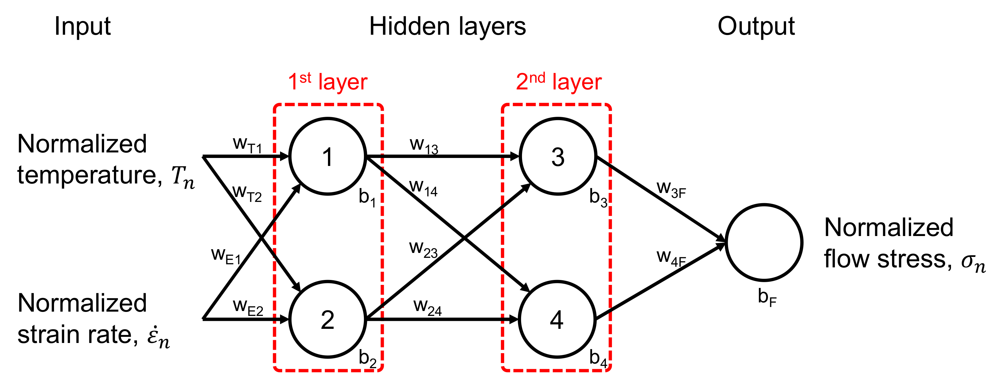
2.4. Structure and Training Method of the Artificial Neural Network

In this paper, an ANN is built for predicting flow stress. The structure of ANN is illustrated in Figure 4. A multilayer perceptron (MLP) is used. There are two hidden layers and a total of four neurons in the hidden layers. When we design the ANN structure, we try to minimize the number of neurons to reduce the complexity of the ANN to avoid overfitting. The experimental dataset (see Section 2.2), including a total of 100 data points of the flow stress, temperature and strain rate, are employed to train the ANN to predict the flow stress. The entire dataset is used to train the ANN in this study. The “lbfgs” optimizer in scikit-learn software [51] is employed as a solver during the training process. A personal computer with a quad-core processor with a clock speed of 2.66 GHz and random access memory (RAM) of 16 GB was used for training the ANN.

The input of the ANN is the normalized temperature, and the normalized strain rate and the output of the ANN is the normalized flow stress. Before the raw data were used, the raw data were scaled by using the following equation. The normalized temperature T_n is calculated by:

$${\mathrm{T}}_{\mathrm{n}}=\frac{\mathrm{T}-350}{250}$$

(3)

where T is the temperature (in °C). The normalized strain rate ${\dot{\mathsf{\epsilon }}}_{\mathrm{n}}$ is calculated by,

$${\dot{\mathsf{\epsilon }}}_{\mathrm{n}}=\frac{{\log }_{10}\dot{\mathsf{\epsilon }}+3}{5}$$

(4)

where $\dot{\mathsf{\epsilon }}$ is the strain rate (in 1/s). The normalized flow stress σ_n is calculated by:

$${\mathsf{\sigma }}_{\mathrm{n}}=\frac{\mathsf{\sigma }}{100}$$

(5)

where σ is strain rate (in MPa). As shown in Figure 4, the input signal X of the proposed ANN is expressed in a vector form given by:

$$\mathrm{X}=\left[\begin{array}{c}{\mathrm{T}}_{\mathrm{n}}\\ {\dot{\mathsf{\epsilon }}}_{\mathrm{n}}\end{array}\right]$$

(6)

The outputs of the 1_st layer is calculated by:

$${\mathrm{Output}}_1=\left[\begin{array}{c}{\mathrm{O}}_1\\ {\mathrm{O}}_2\end{array}\right]=\tanh \left(\left[\begin{array}{cc}{\mathrm{w}}_{\mathrm{T}1}& {\mathrm{w}}_{\mathrm{E}1}\\ {\mathrm{w}}_{\mathrm{T}2}& {\mathrm{w}}_{\mathrm{E}2}\end{array}\right]\left[\begin{array}{c}{\mathrm{T}}_{\mathrm{n}}\\ {\dot{\mathsf{\epsilon }}}_{\mathrm{n}}\end{array}\right]+\left[\begin{array}{c}{\mathrm{b}}_1\\ {\mathrm{b}}_2\end{array}\right]\right)$$

(7)

where O₁ and O₂ are the output of neuron 1 and neuron 2, w_T1, w_T2, w_E1and w_E2 are the weight coefficients, and b₁ and b₂ are the bias of neuron 1 and neuron 2. The outputs of the 2nd layer is calculated by:

$${\mathrm{Output}}_2=\left[\begin{array}{c}{\mathrm{O}}_3\\ {\mathrm{O}}_4\end{array}\right]=\tanh \left(\left[\begin{array}{cc}{\mathrm{w}}_{13}& {\mathrm{w}}_{23}\\ {\mathrm{w}}_{14}& {\mathrm{w}}_{24}\end{array}\right]\left[\begin{array}{c}{\mathrm{O}}_1\\ {\mathrm{O}}_2\end{array}\right]+\left[\begin{array}{c}{\mathrm{b}}_3\\ {\mathrm{b}}_4\end{array}\right]\right)$$

(8)

where O₃ and O₄ are the output of neuron 3 and neuron 4, w₁₃, w₁₄, w₂₃and w₂₄ are the weight coefficients, and b₃ and b₄ are the bias of neuron 3 and neuron 4. The output of the ANN is calculated by:

$${\sigma }_n=\left[\begin{array}{cc}{w}_{3F}& w_{4F}\end{array}\right]\left[\begin{array}{c}{O}_3\\ O_4\end{array}\right]+\left[b_F\right]$$

(9)

where w_3F and w_4F are the weight coefficients, and b_F are the bias in the output layer.

3. Results and Discussion

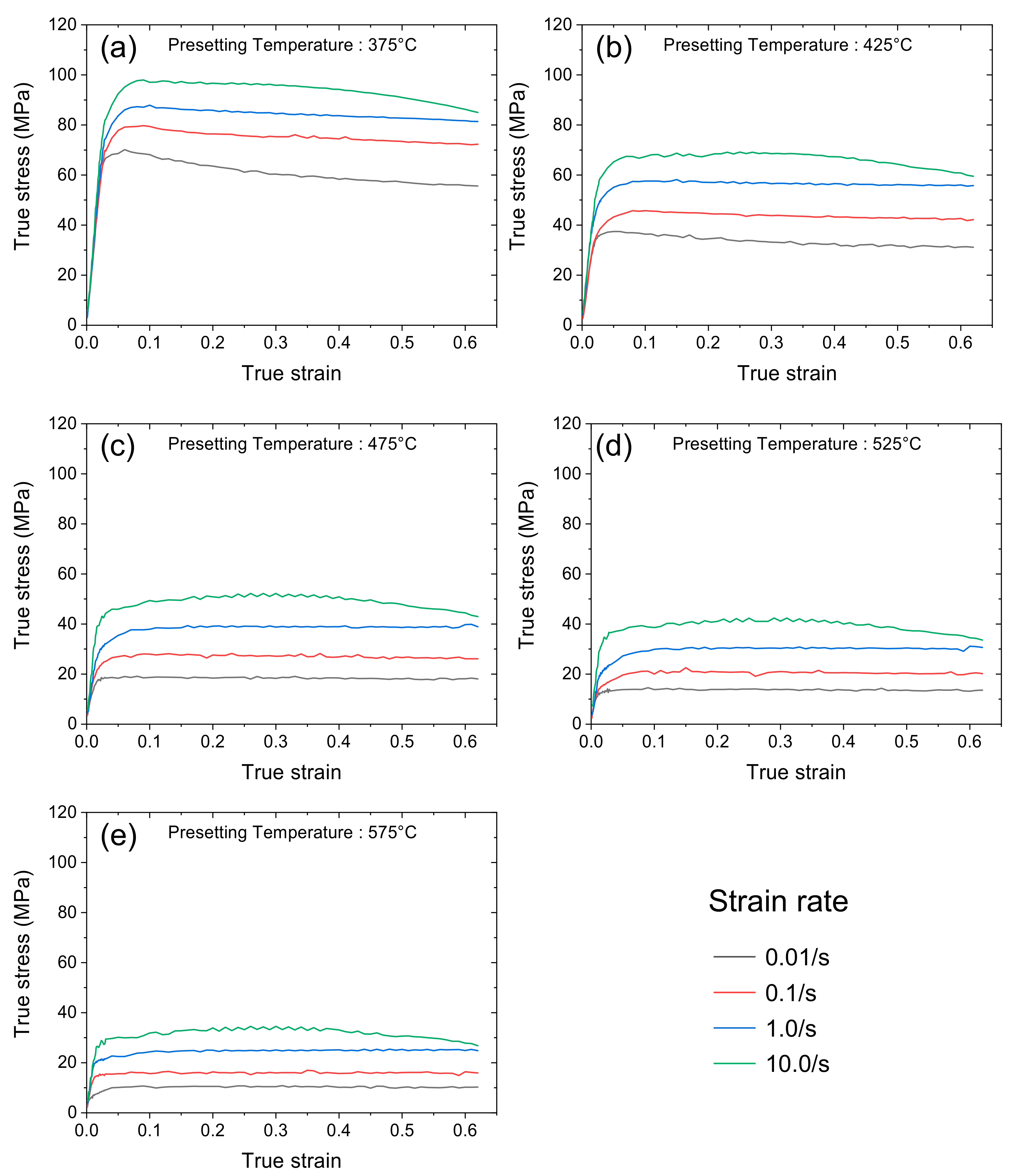
3.1. Measured Stress–Strain Curve

Figure 5 shows the measured stress–strain curve in the hot compression tests for AA6061 at the designed temperatures and strain rates. The strain rates range from 0.01/s to 10.0/s. Figure 5a shows the stress–strain curve at the testing strain rates when the presetting deformation temperature is 375 °C. Figure 5b shows the stress–strain curve at the testing strain rates when the presetting deformation temperature is 425 °C. Figure 5c shows the stress–strain curve at the testing strain rates when the presetting temperature is 475 °C. Figure 5d shows the stress–strain curve at the testing strain rates when the presetting deformation temperature is 525 °C. Figure 5e shows the stress–strain curve at the testing strain rates when the presetting deformation temperature is 575 °C. The flow stress measures the necessary stress that causes plastic deformation. In other words, the flow stress is a measure of the resistance that the metals experience during plastic deformation. It could be found that the shape of the stress–strain curves at different deformation temperatures and different strain rates are quite similar. As shown in Figure 5a–e, a stress–strain curve in the hot compression test generally includes two deformation stages, which are the elastic deformation stage and the plastic deformation stage. The plastic stage starts when the true strain is ~0.05. At the early stage of the plastic deformation, when the strain is less than 0.1, the stress increases gradually as the strain increases. The stress–strain curve tends to be flat at large strains. This is attributed to the softening mechanism of the dynamic recovery and the dynamic recrystallization [52]. Generally, when the strain exceeds 0.2, the stress–strain curve becomes almost independent of strain, as shown in Figure 5.

3.2. Measured Temperature–Strain Curve

Figure 6 shows the measured temperature–strain curve in the above hot compression tests for AA6061 at the designed temperatures and strain rates. The strain rates range from 0.01/s to 10.0/s. Figure 6a shows the temperature–strain curve at the testing strain rates when the presetting deformation temperature is 375 °C. Figure 6b shows the temperature–strain curve at the testing strain rates when the presetting deformation temperature is 425 °C. Figure 6c shows the temperature–strain curve at the testing strain rates when the presetting deformation temperature is 475 °C. Figure 6d shows the temperature–strain curve at the testing strain rates when the presetting deformation temperature is 525 °C. Figure 6e shows the temperature–strain curve at the testing strain rates when the presetting deformation temperature is 575 °C. It could be seen from Figure 6a–e, the temperature fluctuates for a few degrees during the hot compression tests. In the hot compression tests by using Gleeble, the temperature is kept constant by applying variable current through the sample. In Figure 6a, it could be seen that the temperature remains almost constant when the strain rate is 0.01/s or 0.1/s. In contrast, the temperature is elevated as the plastic strain increases when the strain rate is 1.0/s or 10.0/s. When the deformation rate becomes high, the rise of temperature caused by the adiabatic heating due to plastic deformation could become more significant. Similar trends could be found in other cases shown in Figure 6b–e. Although the temperature rise due to the adiabatic heating becomes less significant because of the thermal softening effect, the temperature could deviate from the presetting temperature during the deformation. Therefore, the measured temperature is used in the dataset for determining the constant in the Sellars–Tegart equation and training of the ANN.

It could be found from the above results that temperature is a major influencing factor on the flow stress of AA6061. Figure 7 plots the measured flow stress versus the deformation temperature at different strain rates when the true strain is 0.4. The deformation temperature is taken from the measured temperature–strain curve shown in Figure 6. It could be seen from Figure 7 that the stress decreases with the increase of deformation temperature. For example, when the temperature is close to 375 °C, the flow stress of AA6061 is 58.3 MPa at the strain rate of 0.01/s. When the temperature is close to 575 °C, the flow stress of AA6061 is as low as 10.2 MPa at the strain rate of 0.01/s.

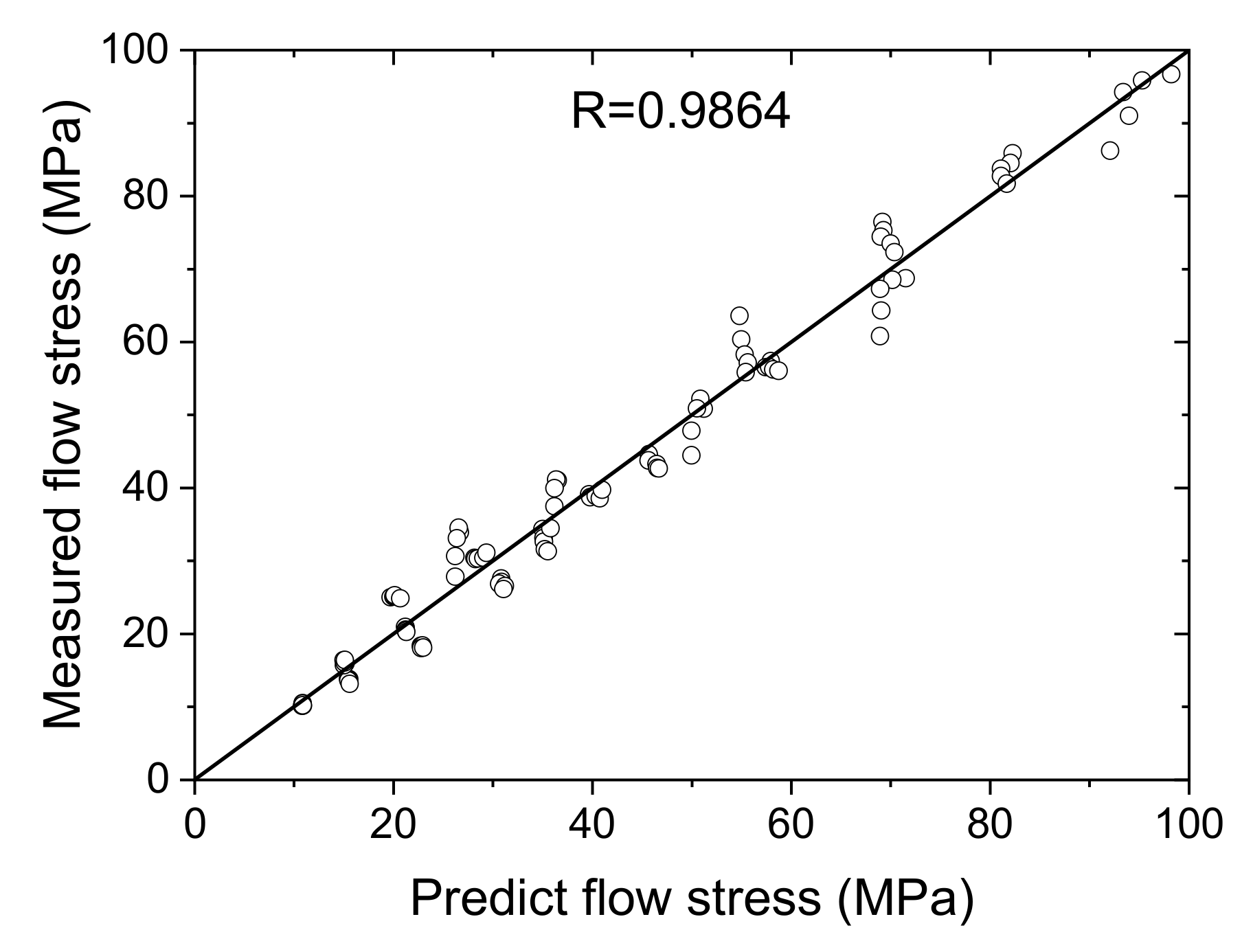
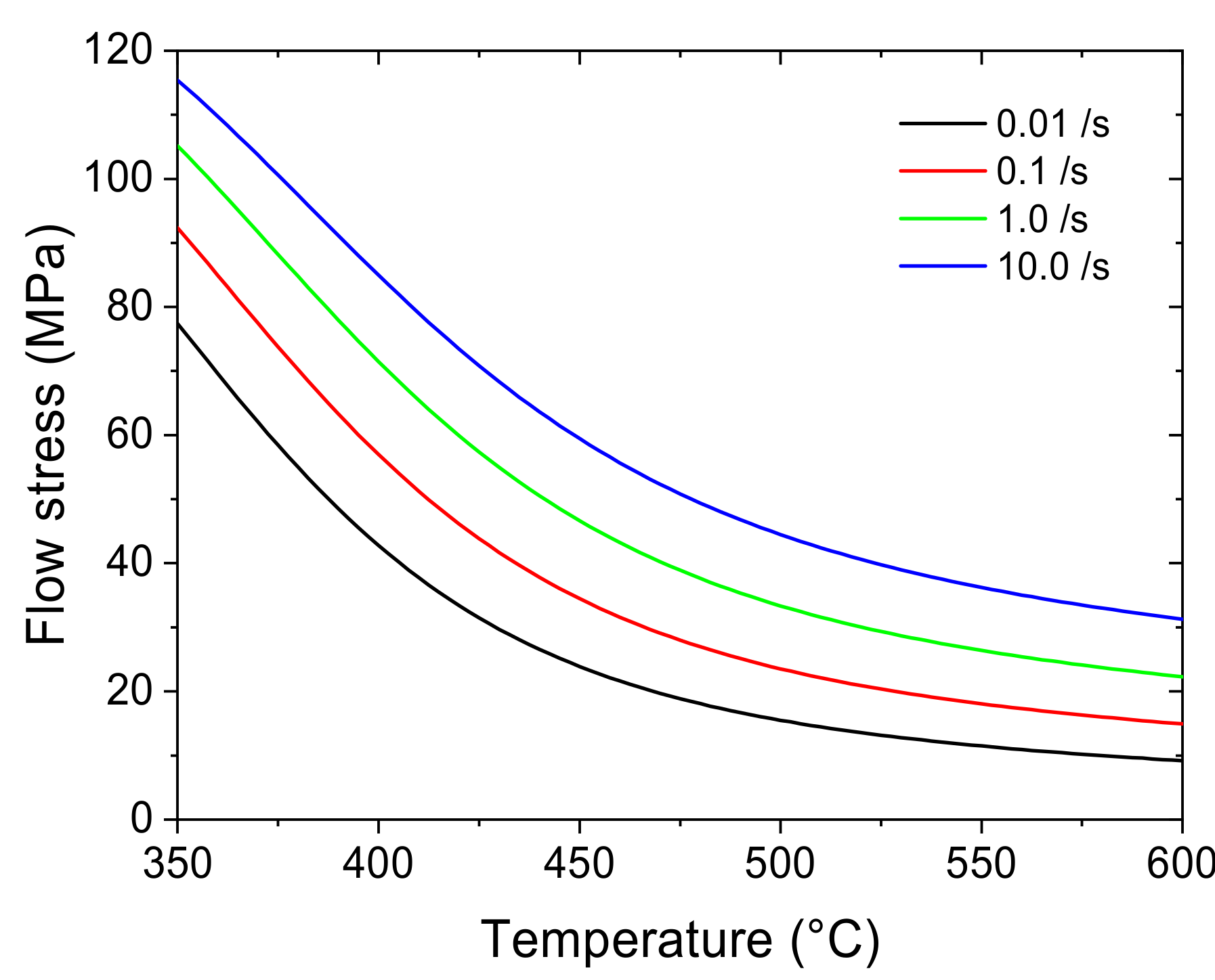
3.3. Predicting the Flow Stress by the Sellars–Tegart Equation

According to Equation (1), the flow stress could be taken as a function of temperature and strain rate. The flow stresses in the dataset built in Section 2.3 are used for the calculation of the constants. The constants in the Sellars–Tegart equation are calculated by using the method proposed in Section 2.3 and listed in

Table 3. Values of constants in the Sellars–Tegart equation for predicting the flow stress.

Parameters	Value
α	0.0173 MPa−1
n	7.25
Q	292 $\mathrm{kJ}/\mathrm{mol}$
A	$1.68\times {10}^{21}$

. The predicted flow stresses at different strain rates are plotted versus temperature in Figure 8. The thermal activation energy, Q, is determined to be 292kJ/mol, as shown in Table 3. This is comparable but lower than the calculated thermal-activation energy in the literature for AA6061, which is 314.304 kJ/mol [28]. It is worth noting that the temperature range for testing in [28] is from 300 °C to 450 °C. The change in the temperature range for testing may influence the value of the thermal-activation energy. Figure 9 shows the correlation between the measured and predicted flow stresses by the Sellars–Tegart equation. The correlation factor is found to be 0.9864. To test the model based on the Sellars–Tegart equation for predicting the flow stress, the root-mean-squared error (RMSE) between the measured and the predicted values of flow stress was calculated by:

$$\mathrm{RMSE}=\sqrt{\frac{1}{m}\sum {\left({\sigma }_{p,i}-{\sigma }_{m,i}\right)}^2}$$

(10)

where m = 100 is the number of data point in the dataset, σ_m,i represents each of the measured flow stress in the dataset and σ_p,i represents each of the predicted flow stress in the dataset. The RMSE regarding the Sellars–Tegart equation is calculated as 3.43 MPa. It is indicated by the comparison between the predicted and measured values of flow stress that the model based on the Sellars–Tegart equations in this paper can predict the flow stress at temperatures ranging from 375 °C to 575 °C and strain rate ranging from 0.01/s to 10/s.

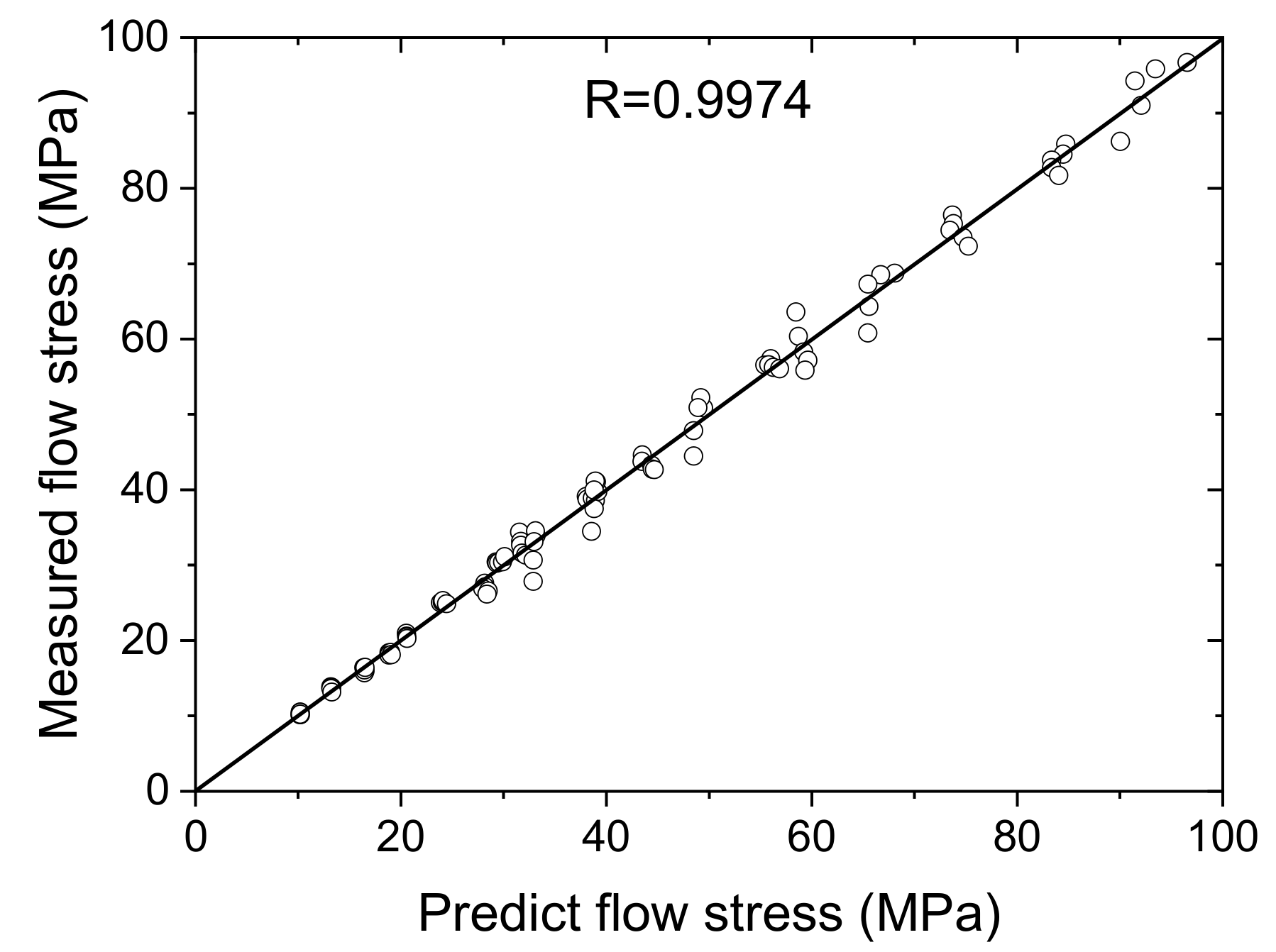
3.4. Predicting the Flow Stress by Artificial Neural Network

Using the method proposed in Section 2.4, the ANN is established to represent the mathematical relationship of the flow stress, the temperature and the strain rate. The flow stresses in the dataset (see Section 2.2) with different temperatures and strain rates are used for training the ANN. After training, all the obtained coefficients in the ANN are listed in

Table 4. Coefficients of the ANN for predicting the flow stress.

Parameters	Value
wT1	−0.15598581
wT2	1.81017239
wE1	0.63329026
wE2	0.04463549
w13	0.27981264
w14	−1.63153269
w23	0.24637079
w24	1.41631146
w3F	0.59353861
w4F	−0.76671464
b1	−0.01082548
b2	0.16777425
b3	0.83656406
b4	−0.14121194
bF	0.28329775

. Figure 10 shows the predicted flow stress by the ANN. Figure 11 shows the correlation between the measured and predicted flow stresses by the Sellars–Tegart equation. The correlation factor is found to be 0.9864. The RMSE between the measured value and the predicted flow stress values by using the proposed ANN is calculated as 1.68 MPa. It could be found from the comparison between the predicted and measured values of flow stress that the ANN established here can predict the flow stress at temperatures ranging from 375 °C to 575 °C and strain rate ranging from 0.01/s to 10/s.

In this paper, the testing temperature is designed to be cover the typical temperature range in FSW, which ranges from 375 °C to 575 °C. The ANN model has more flexibility in the complex fitting relationship than the Sellars–Tegart equation. Therefore, we would suggest using the ANN model if adequate data covering the typical temperature range in FSW is available in the modeling and simulation of FSW. Combining data with an ANN would be a good substation to predict the flow stress for the design and simulation of FSW and similar processes.

4. Conclusions

The purpose of this paper is to report quantitative data and models for the flow stress for the computer simulation of FSW. The experimental flow stress is measured by using hot compression tests. Unlike the current studies, the deformation temperature in this study is designed to cover the typical range during FSW. We report two models, i.e., Sellars–Tegart equation and artificial neural network (ANN), for predicting the flow stress of the commercial 6061 aluminum alloy based on experimental data at typical temperatures during FSW. The root-mean-squared error (RMSE) between the measured and the predicted values are found to be 3.43 MPa for the model based on the Sellars–Tegart equation and 1.68 MPa for the model based on ANN. ANN shows better flexibility than the Sellars–Tegart equation in predicting the flow stress at typical temperatures during FSW. In the future, data together with an ANN would be a substation way to predict the flow stress for the design and simulation of FSW and similar processes.

References

1. Mishra, R.S.; Ma, Z.Y. Friction stir welding and processing. Mater. Sci. Eng. R-Rep. 2005, 50, 1–78. [Google Scholar] [CrossRef]
2. Nandan, R.; DebRoy, T.; Bhadeshia, H. Recent advances in friction-stir welding–process, weldment structure and properties. Prog. Mater. Sci. 2008, 53, 980–1023. [Google Scholar] [CrossRef] [Green Version]
3. Shen, Z.; Ding, Y.; Gerlich, A.P. Advances in friction stir spot welding. Crit. Rev. Solid State Mater. Sci. 2019, 1–78. [Google Scholar] [CrossRef]
4. Meng, X.; Huang, Y.; Cao, J.; Shen, J.; dos Santos, J.F. Recent progress on control strategies for inherent issues in friction stir welding. Prog. Mater. Sci. 2021, 115, 100706. [Google Scholar] [CrossRef]
5. Jandaghi, M.R.; Pouraliakbar, H.; Saboori, A.; Hong, S.I.; Pavese, M. Comparative Insight into the Interfacial Phase Evolutions during Solution Treatment of Dissimilar Friction Stir Welded AA2198-AA7475 and AA2198-AA6013 Aluminum Sheets. Materials 2021, 14, 1290. [Google Scholar] [CrossRef]
6. El Rayes, M.M.; Soliman, M.S.; Abbas, A.T.; Pimenov, D.Y.; Erdakov, I.N.; Abdel-mawla, M.M. Effect of Feed Rate in FSW on the Mechanical and Microstructural Properties of AA5754 Joints. Adv. Mater. Sci. Eng. 2019, 2019, 4156176. [Google Scholar] [CrossRef] [Green Version]
7. Xu, W.F.; Luo, Y.X.; Fu, M.W. Microstructure evolution in the conventional single side and bobbin tool friction stir welding of thick rolled 7085-T7452 aluminum alloy. Mater. Charact. 2018, 138, 48–55. [Google Scholar] [CrossRef]
8. Chen, J.; Ueji, R.; Fujii, H. Double-sided friction-stir welding of magnesium alloy with concave-convex tools for texture control. Mater. Des. 2015, 76, 181–189. [Google Scholar] [CrossRef]
9. Mori, K.-I.; Bay, N.; Fratini, L.; Micari, F.; Tekkaya, A.E. Joining by plastic deformation. CIRP Ann. 2013, 62, 673–694. [Google Scholar] [CrossRef]
10. Chen, G.Q.; Shi, Q.Y.; Li, Y.J.; Sun, Y.J.; Dai, Q.L.; Jia, J.Y.; Zhu, Y.C.; Wu, J.J. Computational fluid dynamics studies on heat generation during friction stir welding of aluminum alloy. Comput. Mater. Sci. 2013, 79, 540–546. [Google Scholar] [CrossRef]
11. Nandan, R.; Roy, G.G.; Lienert, T.J.; Debroy, T. Three-dimensional heat and material flow during friction stir welding of mild steel. Acta Mater. 2007, 55, 883–895. [Google Scholar] [CrossRef]
12. Yu, P.; Wu, C.; Shi, L. Analysis and characterization of dynamic recrystallization and grain structure evolution in friction stir welding of aluminum plates. Acta Mater. 2021, 207, 116692. [Google Scholar] [CrossRef]
13. Zhao, J.; Wu, C.S.; Su, H. Ultrasonic effect on thickness variations of intermetallic compound layers in friction stir welding of aluminium/magnesium alloys. J. Manuf. Process. 2021, 62, 388–402. [Google Scholar] [CrossRef]
14. Zhu, Y.C.; Chen, G.Q.; Chen, Q.L.; Zhang, G.; Shi, Q.Y. Simulation of material plastic flow driven by non-uniform friction force during friction stir welding and related defect prediction. Mater. Des. 2016, 108, 400–410. [Google Scholar] [CrossRef]
15. Long, L.; Chen, G.Q.; Zhang, S.; Liu, T.; Shi, Q.Y. Finite-element analysis of the tool tilt angle effect on the formation of friction stir welds. J. Manuf. Process. 2017, 30, 562–569. [Google Scholar] [CrossRef]
16. Chen, G.; Zhang, S.; Zhu, Y.; Yang, C.; Shi, Q. Thermo-mechanical Analysis of Friction Stir Welding: A Review on Recent Advances. Acta Metall. Sin. 2020, 33, 3–12. [Google Scholar] [CrossRef] [Green Version]
17. He, X.C.; Gu, F.S.; Ball, A. A review of numerical analysis of friction stir welding. Prog. Mater. Sci. 2014, 65, 1–66. [Google Scholar] [CrossRef] [Green Version]
18. Sellars, C.; McTegart, W. On the mechanism of hot deformation. Acta Metall. 1966, 14, 1136–1138. [Google Scholar] [CrossRef]
19. Colegrove, P.A.; Shercliff, H.R. 3-Dimensional CFD modelling of flow round a threaded friction stir welding tool profile. J. Mater. Process. Technol. 2005, 169, 320–327. [Google Scholar] [CrossRef]
20. Pan, W.X.; Li, D.S.; Tartakovsky, A.M.; Ahzi, S.; Khraisheh, M.; Khaleel, M. A new smoothed particle hydrodynamics non-Newtonian model for friction stir welding: Process modeling and simulation of microstructure evolution in a magnesium alloy. Int. J. Plast. 2013, 48, 189–204. [Google Scholar] [CrossRef]
21. Woo, W.; Feng, Z.; Wang, X.L.; Brown, D.W.; Clausen, B.; An, K.; Choo, H.; Hubbard, C.R.; David, S.A. In situ neutron diffraction measurements of temperature and stresses during friction stir welding of 6061-T6 aluminium alloy. Sci. Technol. Weld. Join. 2007, 12, 298–303. [Google Scholar] [CrossRef]
22. Liu, Z.L.; Ji, S.D.; Meng, X.C. Joining of magnesium and aluminum alloys via ultrasonic assisted friction stir welding at low temperature. Int. J. Adv. Manuf. Technol. 2018, 97, 4127–4136. [Google Scholar] [CrossRef]
23. Liu, F.J.; Fu, L.; Chen, H.Y. Effect of high rotational speed on temperature distribution, microstructure evolution, and mechanical properties of friction stir welded 6061-T6 thin plate joints. Int. J. Adv. Manuf. Technol. 2018, 96, 1823–1833. [Google Scholar] [CrossRef]
24. Gerlich, A.; Su, P.; North, T.H. Peak temperatures and microstructures in aluminium and magnesium alloy friction stir spot welds. Sci. Technol. Weld. Join. 2005, 10, 647–652. [Google Scholar] [CrossRef]
25. Alharthi, N.H.; Sherif, E.M.; Taha, M.A.; Abbas, A.T.; Abdo, H.S.; Alharbi, H.F. Influence of Extrusion Temperature on the Corrosion Behavior in Sodium Chloride Solution of Solid State Recycled Aluminum Alloy 6061 Chips. Crystals 2020, 10, 353. [Google Scholar] [CrossRef]
26. Berndt, N.; Frint, P.; Wagner, M.F.X. Influence of Extrusion Temperature on the Aging Behavior and Mechanical Properties of an AA6060 Aluminum Alloy. Metals 2018, 8, 51. [Google Scholar] [CrossRef] [Green Version]
27. Zhao, Q.-L.; Shan, T.-T.; Geng, R.; Zhang, Y.-Y.; He, H.-Y.; Qiu, F.; Jiang, Q.-C. Effect of Preheating Temperature on the Microstructure and Tensile Properties of 6061 Aluminum Alloy Processed by Hot Rolling-Quenching. Metals 2019, 9, 182. [Google Scholar] [CrossRef] [Green Version]
28. Zhang, X.; Wang, X.; Zhang, D. Investigation into Constitutive Equation and Hot Compression Deformation Behavior of 6061 Al Alloy. Teh. Vjesn. 2019, 26, 1376–1382. [Google Scholar] [CrossRef]
29. Colegrove, P.A.; Shercliff, H.R. CFD modelling of friction stir welding of thick plate 7449 aluminium alloy. Sci. Technol. Weld. Join. 2006, 11, 429–441. [Google Scholar] [CrossRef]
30. Colegrove, P.A.; Shercliff, H.R.; Zettler, R. Model for predicting heat generation and temperature in friction stir welding from the material properties. Sci. Technol. Weld. Join. 2007, 12, 284–297. [Google Scholar] [CrossRef] [Green Version]
31. Su, H.; Wu, C.S.; Pittner, A.; Rethmeier, M. Thermal energy generation and distribution in friction stir welding of aluminum alloys. Energy 2014, 77, 720–731. [Google Scholar] [CrossRef]
32. Shi, L.; Wu, C.S.; Gao, S.; Padhy, G.K. Modified constitutive equation for use in modeling the ultrasonic vibration enhanced friction stir welding process. Scr. Mater. 2016, 119, 21–26. [Google Scholar] [CrossRef]
33. Zhao, W.; Wu, C. Constitutive equation including acoustic stress work and plastic strain for modeling ultrasonic vibration assisted friction stir welding process. Int. J. Mach. Tools Manuf. 2019, 145, 103434. [Google Scholar] [CrossRef]
34. Chen, G.Q.; Li, H.; Wang, G.Q.; Guo, Z.Q.; Zhang, S.; Dai, Q.L.; Wang, X.B.; Zhang, G.; Shi, Q.Y. Effects of pin thread on the in-process material flow behavior during friction stir welding: A computational fluid dynamics study. Int. J. Mach. Tools Manuf. 2018, 124, 12–21. [Google Scholar] [CrossRef]
35. Chen, G.; Wang, G.; Shi, Q.; Zhao, Y.; Hao, Y.; Zhang, S. Three-dimensional thermal-mechanical analysis of retractable pin tool friction stir welding process. J. Manuf. Process. 2019, 41, 1–9. [Google Scholar] [CrossRef]
36. Ding, F.J.; Jia, X.D.; Hong, T.J.; Xu, Y.L. Flow Stress Prediction Model of 6061 Aluminum Alloy Sheet Based on GA-BP and PSO-BP Neural Networks. Rare Metal Mater. Eng. 2020, 49, 1840–1853. [Google Scholar]
37. Merayo, D.; Rodriguez-Prieto, A.; Camacho, A.M. Prediction of the Bilinear Stress-Strain Curve of Aluminum Alloys Using Artificial Intelligence and Big Data. Metals 2020, 10, 904. [Google Scholar] [CrossRef]
38. Huang, C.; Jia, X.; Zhang, Z. A Modified Back Propagation Artificial Neural Network Model Based on Genetic Algorithm to Predict the Flow Behavior of 5754 Aluminum Alloy. Materials 2018, 11, 855. [Google Scholar] [CrossRef] [PubMed] [Green Version]
39. Khalaj, G.; Azimzadegan, T.; Khoeini, M.; Etaat, M. Artificial neural networks application to predict the ultimate tensile strength of X70 pipeline steels. Neural Comput. Appl. 2013, 23, 2301–2308. [Google Scholar] [CrossRef]
40. Pouraliakbar, H.; Hosseini Monazzah, A.; Bagheri, R.; Seyed Reihani, S.M.; Khalaj, G.; Nazari, A.; Jandaghi, M.R. Toughness prediction in functionally graded Al6061/SiCp composites produced by roll-bonding. Ceram. Int. 2014, 40, 8809–8825. [Google Scholar] [CrossRef]
41. Winiczenko, R.; Górnicki, K.; Kaleta, A.; Janaszek-Mańkowska, M. Optimisation of ANN topology for predicting the rehydrated apple cubes colour change using RSM and GA. Neural Comput. Appl. 2018, 30, 1795–1809. [Google Scholar] [CrossRef] [Green Version]
42. Hwang, Y.-M.; Kang, Z.-W.; Chiou, Y.-C.; Hsu, H.-H. Experimental study on temperature distributions within the workpiece during friction stir welding of aluminum alloys. Int. J. Mach. Tools Manuf. 2008, 48, 778–787. [Google Scholar] [CrossRef]
43. Assidi, M.; Fourment, L.; Guerdoux, S.; Nelson, T. Friction model for friction stir welding process simulation: Calibrations from welding experiments. Int. J. Mach. Tools Manuf. 2010, 50, 143–155. [Google Scholar] [CrossRef]
44. Feng, Z.; Wang, X.L.; David, S.A.; Sklad, P.S. Modelling of residual stresses and property distributions in friction stir welds of aluminium alloy 6061-T6. Sci. Technol. Weld. Join. 2007, 12, 348–356. [Google Scholar] [CrossRef]
45. Zhang, J.Q.; Shen, Y.F.; Li, B.; Xu, H.S.; Yao, X.; Kuang, B.B.; Gao, J.C. Numerical simulation and experimental investigation on friction stir welding of 6061-T6 aluminum alloy. Mater. Des. 2014, 60, 94–101. [Google Scholar] [CrossRef]
46. Sun, Z.; Wu, C.S. A numerical model of pin thread effect on material flow and heat generation in shear layer during friction stir welding. J. Manuf. Process. 2018, 36, 10–21. [Google Scholar] [CrossRef]
47. Zhai, M.; Wu, C.; Su, H. Influence of tool tilt angle on heat transfer and material flow in friction stir welding. J. Manuf. Process. 2020, 59, 98–112. [Google Scholar] [CrossRef]
48. Gerlich, A.; Yamamoto, M.; North, T.H. Strain rates and grain growth in Al 5754 and Al 6061 friction stir spot welds. Metall. Mater. Trans. A-Phys. Metall. Mater. Sci. 2007, 38A, 1291–1302. [Google Scholar] [CrossRef]
49. Liu, X.C.; Wu, C.S.; Padhy, G.K. Characterization of plastic deformation and material flow in ultrasonic vibration enhanced friction stir welding. Scr. Mater. 2015, 102, 95–98. [Google Scholar] [CrossRef]
50. Lei, B.W.; Chen, G.Q.; Liu, K.H.; Wang, X.; Jiang, X.M.; Pan, J.L.; Shi, Q.Y. Constitutive Analysis on High-Temperature Flow Behavior of 3Cr-1Si-1Ni Ultra-High Strength Steel for Modeling of Flow Stress. Metals 2019, 9, 42. [Google Scholar] [CrossRef] [Green Version]
51. Pedregosa, F.; Varoquaux, G.; Gramfort, A.; Michel, V.; Thirion, B.; Grisel, O.; Blondel, M.; Prettenhofer, P.; Weiss, R.; Dubourg, V.; et al. Scikit-learn: Machine Learning in Python. J. Mach. Learn. Res. 2011, 12, 2825–2830. [Google Scholar]
52. Prasad, Y.; Sasidhara, S. Hot Working guide: A Compendium of Processing Maps; ASM International: Almere, The Netherlands, 1997. [Google Scholar]
Figure 1. Specimen and configuration of the hot compression tests. (a) The cylinder specimen is connected with a thermocouple before the tests; (b) The configuration of the tests.
Metals 11 00804 g001
Figure 2. Thermomechanical history during the hot compression tests. (a) Temperature history; (b) strain history.
Metals 11 00804 g002
Figure 3. Geometry of the sample. (a,b) presents the sample before compression. (c,d) shows the sample after compression.
Metals 11 00804 g003
Figure 4. Structure of the artificial neural network for predicting the flow stress.
Metals 11 00804 g004
Figure 5. Measured stress–strain curves of AA6061 aluminum. The experiment data at different deformation conditions are grouped by the presetting temperature (a) 375 °C, (b) 425 °C, (c) 475 °C, (d) 525 °C and (e) 575 °C.
Metals 11 00804 g005
Figure 6. Measured temperature–strain curves during hot compression tests of AA6061 aluminum. The experiment data at different deformation conditions are grouped by the presetting temperature (a) 375 °C, (b) 425 °C, (c) 475 °C, (d) 525 °C and (e) 575 °C.
Metals 11 00804 g006
Figure 7. Influence of temperature on the measured flow stress of AA6061-T6 (true strain = 0.4).
Metals 11 00804 g007
Figure 8. Predicted flow stresses by the Sellars–Tegart equation.
Metals 11 00804 g008
Figure 9. Correlation between the measured flow stresses and predicted flow stresses by the Sellars–Tegart equation.
Metals 11 00804 g009
Figure 10. Predicted flow stresses by the artificial neural network.
Metals 11 00804 g010
Figure 11. Correlation between the measured flow stresses and predicted flow stresses by an artificial neural network.
Metals 11 00804 g011