Multi–interface isothermal and nonisothermal kinetics experiments can further determine the influence of CO
2 concentration on the reduction rate in the CVTO smelting process. The nonisothermal kinetic process can reflect the complexity and activity of the interfacial reaction at different stages in the experiments of the softening–melting–dripping characteristics. As shown in
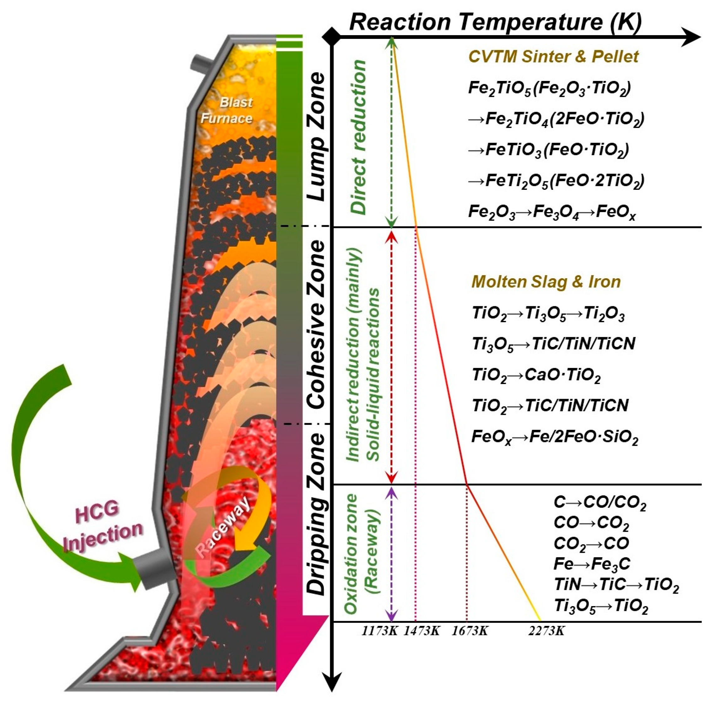
Figure 5, the results of nonisothermal kinetics show that the weight change is synchronized with the softening–melting–dripping experiments. It can be found that as the temperature increases, the nonisothermal kinetics curve shows a nonlinear change, which means that complex multi–interface reactions may occur simultaneously during the CVTO reduction smelting process, such as the gas–solid reaction in the lump zone, the solid–solid/gas reaction in the softening zone, and the liquid–liquid/solid/gas reaction in the dripping zone.
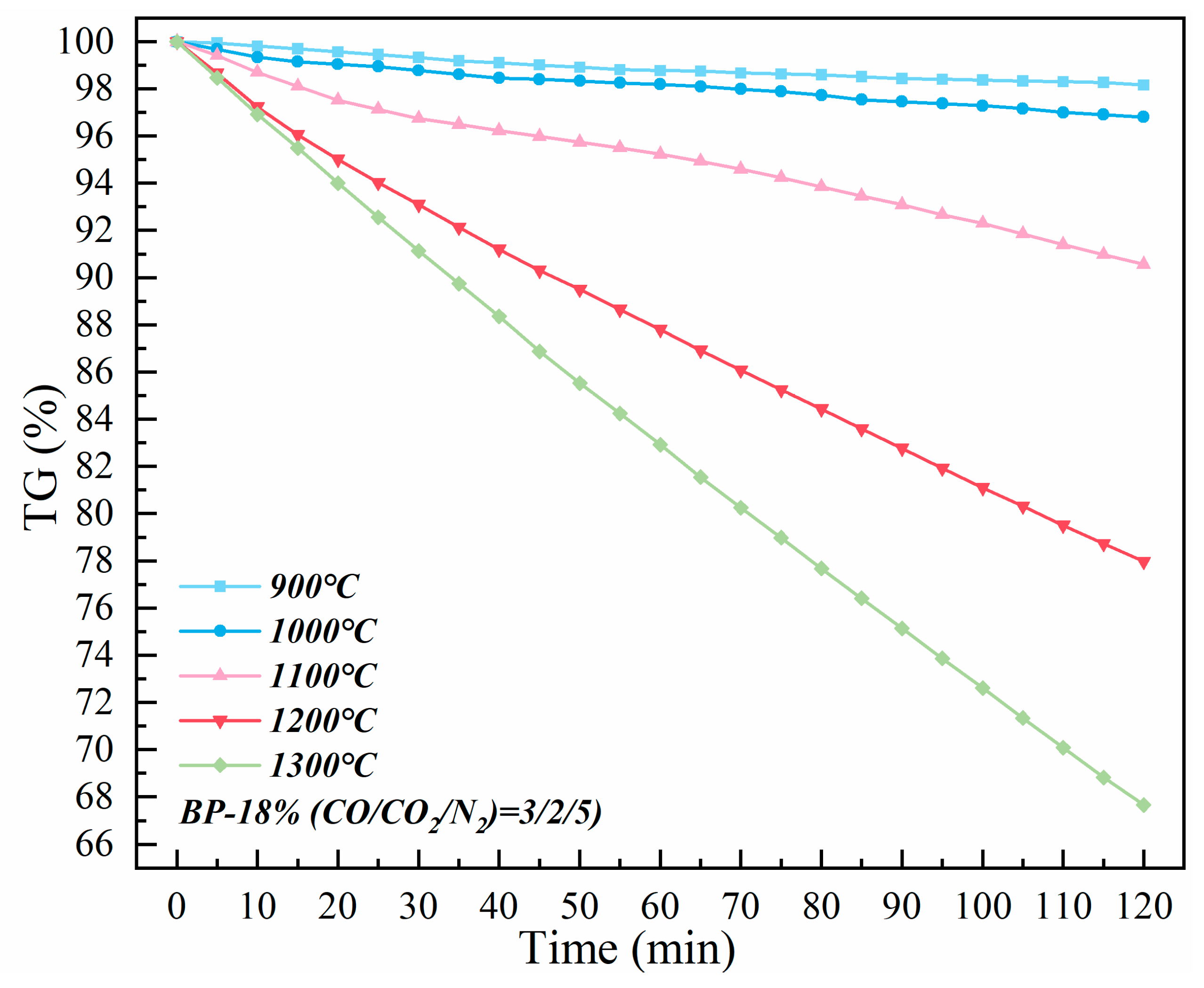
Figure 6 shows the weight change of the sample’s multi–interface isothermal kinetics. When the side temperature increases from 900 °C to 1300 °C, it is estimated that the corresponding core temperature rises from 800 °C to 1200 °C. The experimental results of isothermal kinetics correspond to the reaction stages of the lump zone and the softening zone in the softening–melting–dripping characteristic experiments. The isothermal kinetics curve shows a linear trend, which indicates that the gas–solid reaction and the solid–solid interface reaction that mainly occur in the lump zone and the softening zone may not be restricted by the diffusion law. Therefore, it can be considered that the weight loss of the charge is caused by complex multi–interface reactions, and the valuable metal oxides may also participate in the reoxidation reaction in the reduction process.
In order to further analyze the nonisothermal and isothermal kinetics curves, the weight loss rate
α can be set to indicate the reduction rate of the charge, and its definition is shown in Equation (1).
where Δ
m is the weight loss of the sample, and m
0 is the original weight of the sample. According to the Avrami–Erofeev model (Equation (2)), it can be judged that the reduction process of the sample conforms to the
n–order reaction.
where
k is the reaction rate constant,
t is the time (min), and n is the Avrami exponent.
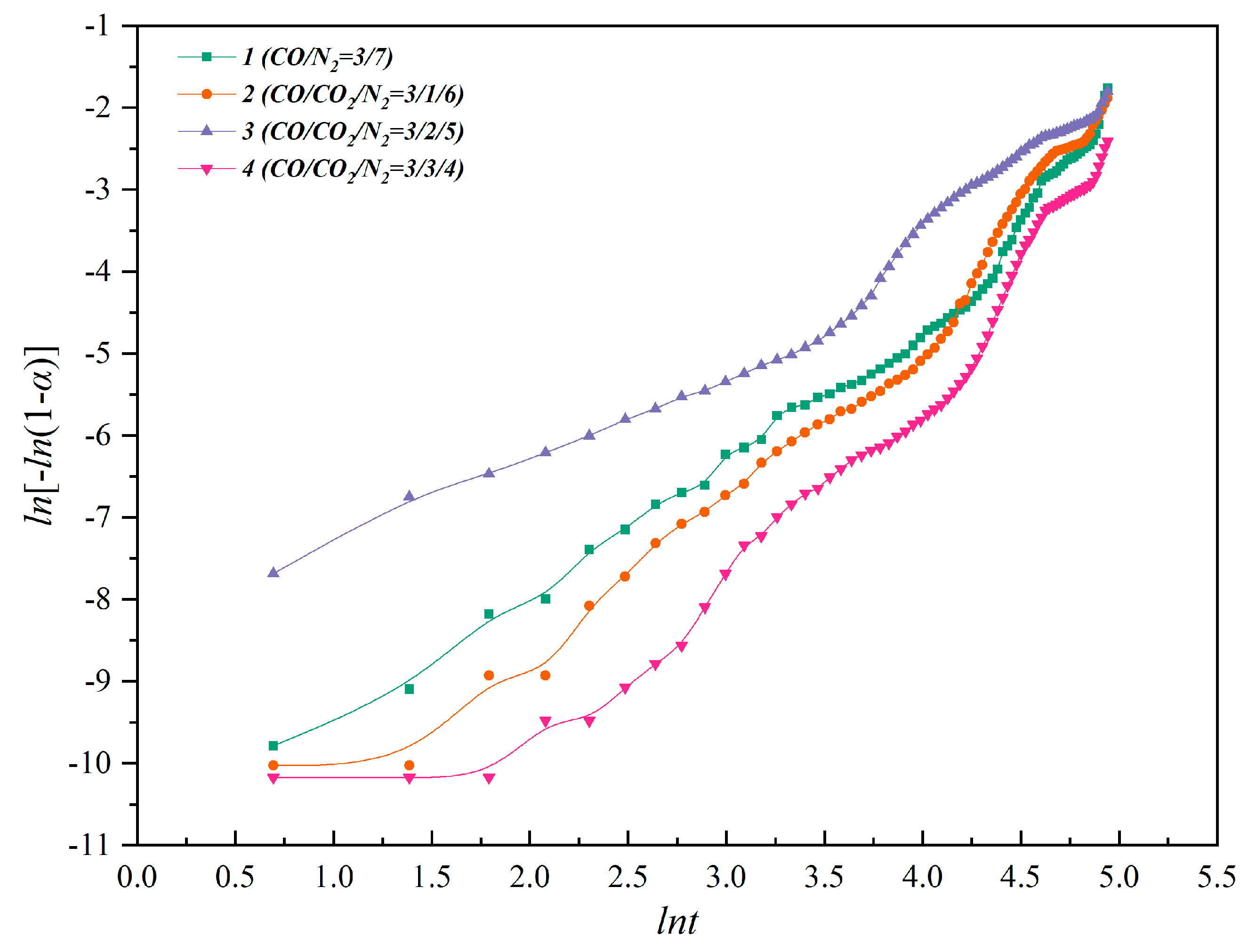
Figure 7 and
Figure 8 show the mapping and fitting of ln [−ln (1 −
α)] − ln
t to nonisothermal and isothermal kinetics, respectively.
Table 2 and
Table 3 are the ln–ln fitting parameters of non–isothermal and isothermal kinetics, respectively. The slope of the fitted line represents the Avrami exponent
n. The fitting slope of ln–ln for nonisothermal kinetics is between 1.3 and 2.6, while the fitting slope of ln–ln for isothermal kinetics is between 0.67 and 1.02. Therefore, according to the commonly used kinetics models and the
n value in
Table 4, the CG
2, A
2, and A
3 models can be used to describe the nonisothermal reduction kinetics process of CVTO, which means that the reduction kinetics model is more suitable for the phase interface reaction model than the random 3D/2D unreacted core model as the concentration of the injected CO
2 increases. In addition, the isothermal reduction kinetics process of CVTO is more in line with the D
1, R
1, and CG
3 models, which means that it may also be suitable for a diffusion model at temperatures where chemical reactions are not active [
13,
15,
16,
17,
18,
19,
20,
25].
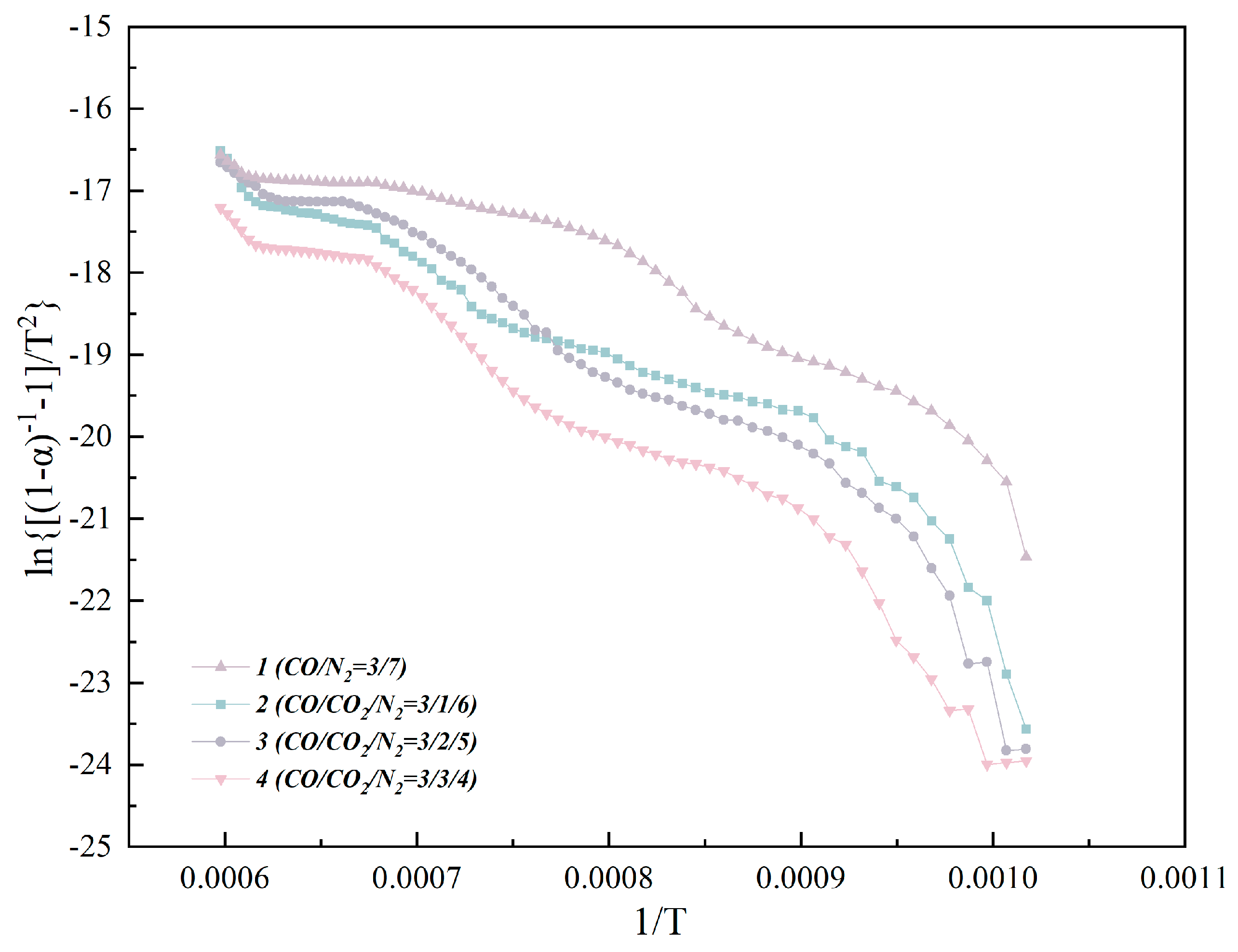
The activation energy of nonisothermal kinetics is generally solved by the Coats–Redfern equation. When
n ≠ 1, the C–R equation is as follows:
where β is the heating rate (K/min),
R is the ideal gas constant 8.314 J·mol
−1·K
−1, and
T is the reduction temperature (K). ln {[1 − (1 −
α)1 − n]/ [(1 − n)
T2]} vs. 1/
T is plotted in
Figure 9. As shown in
Table 5, as the concentration of the injected CO
2 increases, the apparent activation energy reaches the minimum value of 75.58 kJ·mol
−1 when CO
2 is 20 vol.%, which means that injecting an appropriate concentration of CO
2 can also effectively promote the smelting process of CVTO.
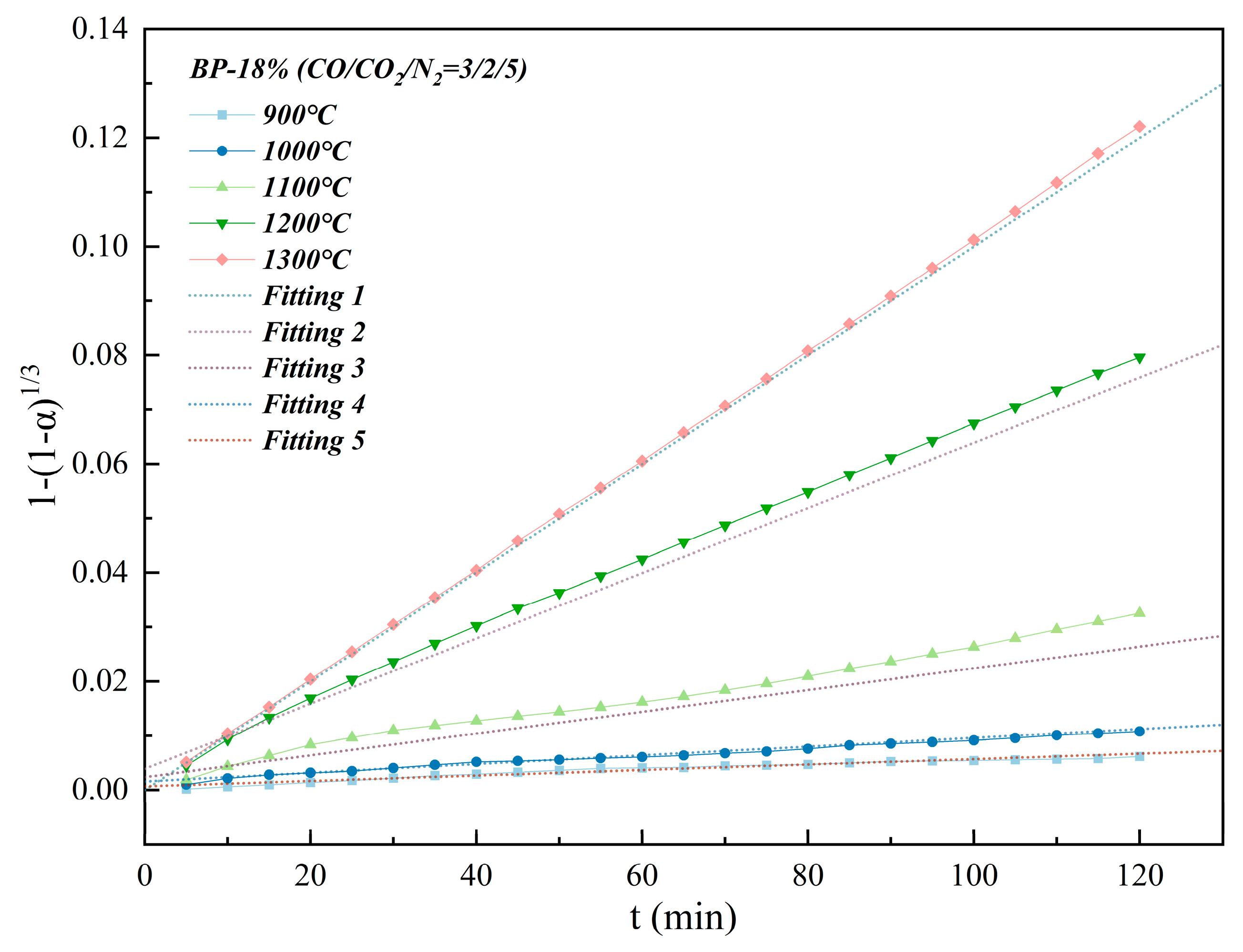
For the activation energy calculation of isothermal kinetics, according to
Table 3 and
Table 4, it can be seen that the isothermal reduction process satisfies the CG
3 model. Therefore, the weight loss rate
α of the isothermal reduction process is fitted according to 1 − (1 −
α)
1/3 −
t, and the result is shown in
Figure 10. The slope of the fitted straight line is the
k value, and the fitting parameters of the isothermal reduction kinetics are shown in
Table 6.
According to the Arrhenius equation (Equation (4)), ln
k and 1/
T can be further fitted, and the fitted straight line is shown in
Figure 11. The slope of the fitted straight line can be solved according to Equation (4), and the apparent activation energy of the isothermal kinetics process is 121.93 kJ·mol
−1. When the apparent activation energy is greater than 400 kJ·mol
−1, the restrictive step is determined by the interface chemical reaction. When the apparent activation energy is less than 150 kJ·mol
−1, the restrictive step is controlled by diffusion. Therefore, the restrictive step of this isothermal kinetics process is mainly determined by diffusion.


