Article

Coupled Modeling Approach for Laser Shock Peening of AA2198-T3: From Plasma and Shock Wave Simulation to Residual Stress Prediction

1
Institute of Product and Process Innovation, Leuphana University of Lüneburg, Universitätsallee 1, 21335 Lüneburg, Germany
2
Institute of Materials Mechanics, Helmholtz-Zentrum Hereon, Max-Planck-Straße 1, 21502 Geesthacht, Germany
3
Modeling and Simulation, Department of Electric Power Engineering, South Westphalia University of Applied Science, Lübecker Ring 2, 59494 Soest, Germany
*
Authors to whom correspondence should be addressed.
Metals 2022, 12(1), 107; https://doi.org/10.3390/met12010107
Submission received: 6 December 2021 / Revised: 24 December 2021 / Accepted: 26 December 2021 / Published: 6 January 2022
(This article belongs to the Special Issue Laser Peening for Improving Fatigue Properties of Aluminium Alloys)

Abstract

:
Laser shock peening (LSP) is a surface modification technique to improve the mechanical properties of metals and alloys, where physical phenomena are difficult to investigate, due to short time scales and extreme physical values. In this regard, simulations can significantly contribute to understand the underlying physics. In this paper, a coupled simulation approach for LSP is presented. A global model of laser–matter–plasma interaction is applied to determine the plasma pressure, which is used as surface loading in finite element (FE) simulations in order to predict residual stress (RS) profiles in the target material. The coupled model is applied to the LSP of AA2198-T3 with water confinement, 3 × 3 mm 2 square focus and 20 ns laser pulse duration. This investigation considers the variation in laser pulse energy (3 J and 5 J) and different protective coatings (none, aluminum and steel foil). A sensitivity analysis is conducted to evaluate the impact of parameter inaccuracies of the global model on the resulting RS. Adjustment of the global model to different laser pulse energies and coating materials allows us to compute the temporal pressure distributions to predict RS with FE simulations, which are in good agreement with the measurements.

1. Introduction

Nowadays, different methods of material surface improvement are available and applied in industry, such as ultrasonic impact treatment [1], shot peening [2] or laser shock peening (LSP) [3]. These techniques allow us to enhance the material performance regarding the fatigue, corrosion and wear resistance of structures and components of, e.g., aircraft or nuclear reactors [3,4].
Within this study, LSP is investigated. It has been described as a process where short laser pulses with a high intensity are used to vaporize the surface layer of a target material or a coating. This vapor is turned into a high-temperature [5] and high-pressure plasma [6], which induces a mechanical shock wave within the material during its expansion; see Figure 1. The propagating shock waves cause local plastic deformation, which results in residual stresses (RS) in the target material [3]. For instance, due to the higher and deeper penetration depth of compressive RS, LSP is a potential substitute for conventional shot peening processes [7].
The generation of high-pressure shock waves in materials by intense laser pulses was first demonstrated by Askaryan and Moroz in 1963 [8]. Shortly thereafter, White [9] experimentally observed this process and concluded that short laser pulses with high intensity can be used to generate acoustic waves in a target material. Further investigations in the mode of direct ablation, where the irradiated target is in a vacuum and the plasma freely expands, are mainly motivated by inertial confinement fusion (ICF) studies [10]. It has been shown that high pressures in ICF can be obtained mainly by varying the incident laser intensity [11]. Furthermore, in this regime, the plasma pressure temporal profile is approximately equal to the laser pulse profile, due to the rapid cooling of the plasma bulk by its adiabatic expansion in vacuum conditions. Both the duration and amplitude of the obtained plasma pressure can be increased by application of a laser-transparent overlay. The usage of such a confinement was introduced by Anderholm [12]. O’Keefe et al. [13] experimentally observed increased peak pressures in the confined case, investigating aluminum alloys and stainless steel. Fairand et al. [14] showed comparisons between measured and calculated pressures, including the effects of different transparent overlays and target absorber materials. It was concluded that significant improvements in the size and duration of a stress wave can be achieved by confinement techniques.
The success of the first experiments with laser-transparent overlays led to the further exploration and development of LSP of metals. Due to the fact that LSP is a highly non-linear process with short-time events, involving a large number of adjustable process parameters, it is difficult to optimize this process based on experiments alone. Additionally, the extreme values of the occurring physical quantities are difficult to measure experimentally, i.e., shock wave propagation and plasma formation. Therefore, a number of studies have been published concerning simulations of LSP at confined regimes [15,16,17,18,19,20,21,22,23,24,25,26,27,28,29,30]. However, the majority of these works are dedicated mostly to finite element (FE) simulations to predict the RS state after LSP using simplified approaches for pressure loading identification, e.g., assumptions of spatial uniformity and linear temporal behavior of the pressure [15,16,17,18,19,20,21,22,23,24,25]. Applying a laser–matter–plasma model allows us to determine the pressure distributions at the material surface, which provides more realistic profiles.
Different approaches to plasma modeling within LSP simulation exist. Pirri et al. [31] proposed one of the first models based on laser-supported combustion wave description. However, this model was applicable only for low-intensity laser pulses and regimes with no confinement. The currently most widely used model [19,20,21,22,23,24,25,26,27] was introduced by Fabbro et al. [27]. This simple analytical model can be applied to confined regimes, but it does not consider any mass or energy exchange within the system, contains experimentally identified parameters and is mainly applied to identify simply the pressure at the material surface. Besides this, the model of Fabbro et al. [27] does not include the effect of different coatings. An advanced model, formulated by Wu et al. [28], includes a detailed description of the occurring processes, taking into account mass and energy flows from material and confinement, and deals only with variables, which are calculated based on related physical phenomena. However, this model does not describe the shock propagation process and also requires large computational effort. More recent thermal models [32,33] properly describe the vaporization of the material surface based on the Hertz–Knudsen equation and vapor breakdown, but no mass or energy transport from a confinement is considered. In addition, no effects of the propagating shock waves are presented. The HELIOS code [29] could be a suitable alternative to the mentioned models, as it contains a precise two-temperature model to describe plasma and shock wave behavior without experimental parameters and is coupled with a user-friendly interface. Although this commercially available code allows us to identify a number of different process parameters, it also requires additional PROPACEOS data [34] and SESAME tables [35] for correct material property description. Therefore, the global model proposed by Zhang et al. [30] is a good compromise between simplicity and accuracy of LSP description. The model allows to identify time-dependent plasma and shocked region parameters, which can be used to study and optimize the process, taking into account mass flows between metal, plasma and confinement.
Time-dependent plasma pressures obtained by all these different models can be used in subsequent FE simulations to predict the RS state of the target material. This process can be split into two phases. The first phase is the pulse phase, where the shock wave causes plastic deformation in the material. The second phase, the relaxation phase, deals with the relaxation of the system, where the time-dependent stress variations decrease and the equilibrium stress state is determined. In particular, the relaxation phase is simulated differently by several authors. The work of Braisted and Brockman [18] can be seen as the first LSP process simulation based on the FE method, predicting the resulting RS after a certain pressure loading at the surface. While the pulse phase is simulated with an explicit solver, an implicit (static) solver is used for the relaxation phase to calculate the equilibrium stress state. In contrast, for example, Bahmare et al. [36] used an explicit solver for the relaxation phase with added artificial damping to decrease the simulation time. The aim is to calculate a state that is close enough to equilibrium.
The material strain rate can reach values up to 10 6 s 1 during LSP [37]. However, the material behavior at such high strain rates is not exactly known. This may lead to inaccuracies in terms of material modeling during the RS prediction. Amachinta et al. [38] compared different material models for LSP process simulation and concluded that the Johnson–Cook model [39] provides the most reasonable results regarding RS prediction. This conclusion is supported for an investigation of aluminum and titanium alloys by Langer et al. [40].
In this paper, the influence of different coating materials on the RS profiles in the aluminum alloy AA2198 in T3 condition at two laser pulse energies is investigated. A schematic of the applied simulation scheme, including the comparison of predicted and experimentally determined RS, is depicted in Figure 2. The laser–matter–plasma interaction is described by the global model of Zhang et al. [30], where input parameters (laser and material properties) yield temporal distributions of physical quantities in water, metal and plasma. The resulting temporal plasma pressure distributions are applied as surface pressure loadings in the FE simulations, following the simulation approach presented in Keller et al. [41], in order to obtain RS distributions within the target material. Unknown plasma parameters are identified based on a comparison between predicted and experimentally determined RS for one experimental scenario. Finally, the global model is applied to different coating materials and two laser pulse energies. RS predictions, based on calculated pressure profiles and experimentally determined RS, show good agreement, indicating that the proposed simulation scheme is applicable for LSP description.

2. Materials and Methods

2.1. Experimental Parameters

In this work, experiments were performed with an Nd:YAG laser (Quantel Laser by Lumibird, Les Ulis, France) with a wavelength of 1064 nm. Laser pulse energies of 3 J and 5 J with the full-width-at-half-maximum (FWHM) of T = 20 ns and a square laser focus with a size of F = 3 × 3 mm 2 were used. Laser pulses were applied with the frequency of 10 Hz. As shown in Figure 3, the used laser provides a non-symmetric temporal profile with the total pulse duration T L of 80 ns. The spatial laser intensity distribution is almost constant over the square spot.
In all LSP experiments, AA2198 sheet material in T3 temper condition, i.e., solution heat-treated and cold-worked, with a sample size of 80 mm × 40 mm × 5 mm , was used. A rectangular peening patch with a size of 15 × 15 mm 2 was applied to analyze the effect of LSP. Laser pulses were arranged in columns that were shot in the same direction. Different surface conditions (no coating, aluminum foil and steel foil) were investigated to study the influence on plasma pressure and RS distribution. Water as a transparent overlay was sprayed above the peened area in order to form a laminar water curtain to have a laser-transparent medium. The experiments were conducted with no overlapping of treated areas. After LSP treatment, the RS state within the material was determined by the measurement system Prism by Stresstech (Rennerod, Germany), which is based on an incremental hole drilling technique and electronic speckle pattern interferometry [42]. A drill diameter of 2 mm was used. RS determinations were repeated at least three times. Results shown in this work represent the average value of these stress determinations, where the experimental scatter represents the minimum and maximum value determined at the respective depth. For more details on the experimental set-up, the interested reader is referred to Keller et al. [41].

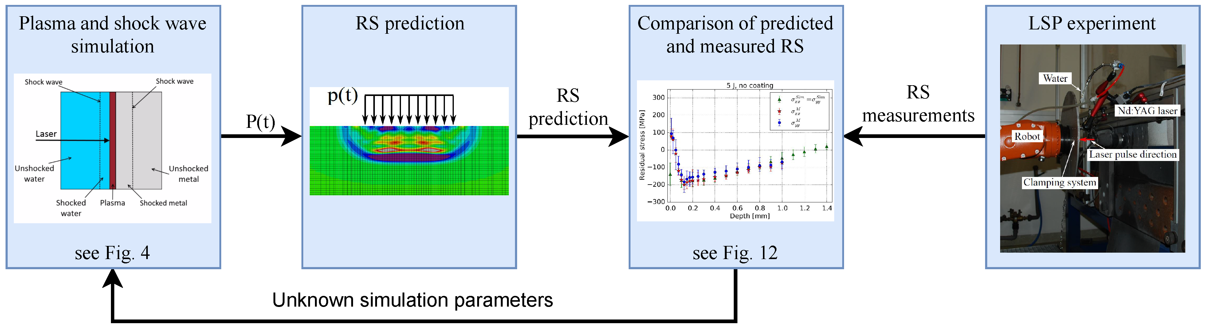
2.2. Simulation Scheme

As outlined in Figure 2, the simulation scheme consists primarily of two main ingredients. At first, a global plasma model is used to determine the resulting pressure pulse due to the laser pulse. The pressure pulse is subsequently used in the FE simulation to predict the RS distribution. Both models are illustrated in detail in the following.

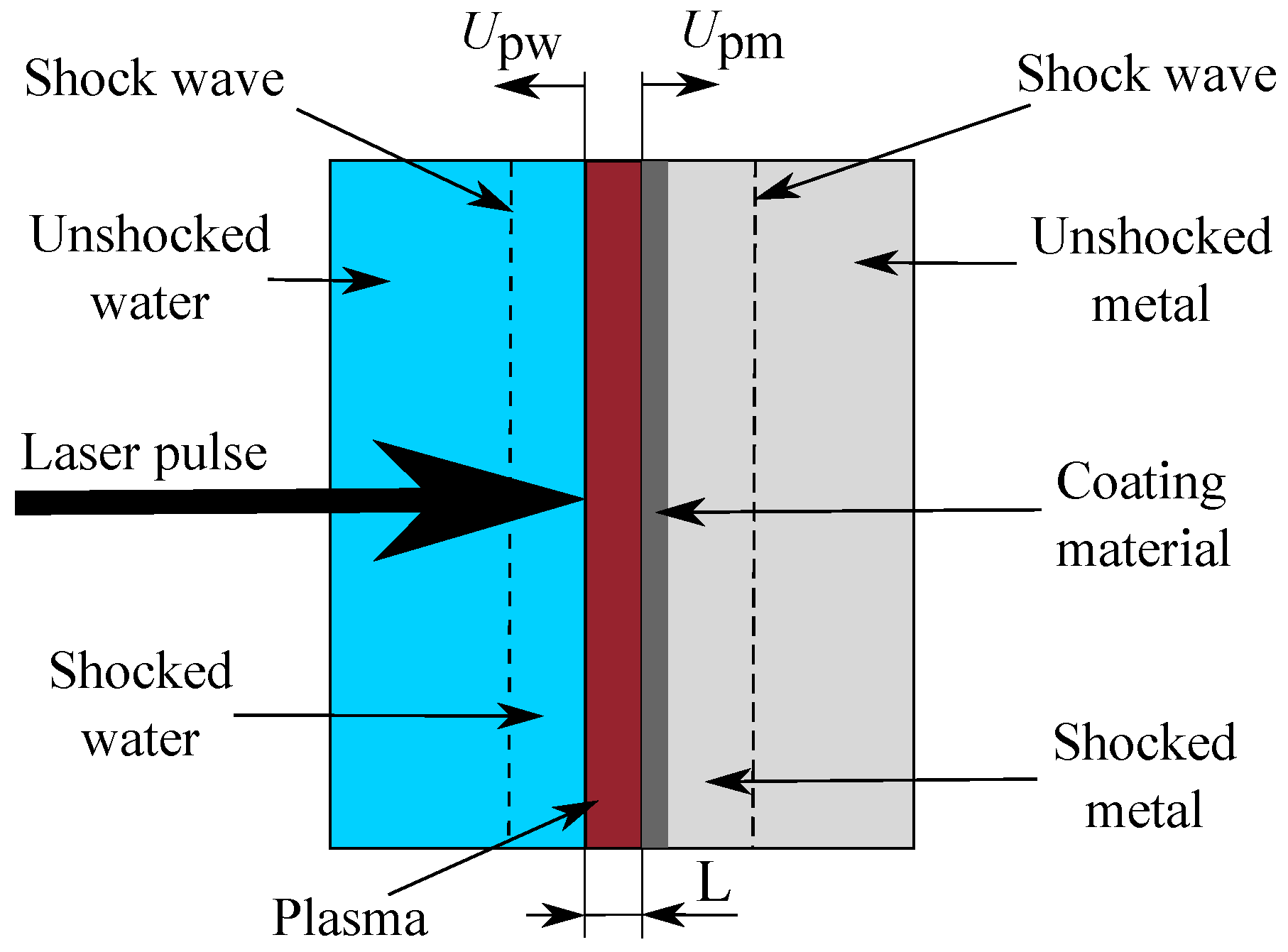
2.2.1. Global LSP Model

To determine the plasma pressure depending on laser parameters and material properties, Zhang et al. [30] proposed a global model for microscale LSP, i.e., laser focus diameter ≈12 μ m, for a metallic sample immersed in a container with water. The thickness of the water layer above the sample was approximately 3 mm. Due to the assumptions of a plasma expansion only in the axial direction and uniform parameter distributions in the radial direction [30], the model is also applicable for larger focus sizes. Besides this, a small thickness of a shocked water region (less than 1 mm), which does not exceed the total water layer thickness at the early stages of shock wave propagation (first 300 ns), allows us to apply the global model also to water curtain confinement. In this regard, in the current research, the model was applied to the LSP of aluminum with a focus size in the mm range, covered with different coating materials and a thin (≈1 mm) water curtain.
For simplicity, five separate interacting regions—see Figure 4—are considered within the model: unshocked and shocked water, unshocked metal, shocked metal with a protecting coating and the plasma. Due to the assumption that the coating layer is thin and well coupled with the target material, all the properties of shocked metal and coating are assumed equal, except the mass density [30]. All unshocked properties of water and metal are known; see Table 1.
The relation between the shocked (i) and unshocked (i0) properties of water (i = w), as well as metal (i = m), are represented by mass (1), momentum (2) and energy (3) conservation laws and coupled with shock speed constitutive relations (4) as follows:
ρ i 0 ρ i = 1 U i D i ,
P i P i 0 = ρ i 0 D i U i ,
E i + U i 2 2 = P i + P i 0 2 1 ρ i 0 1 ρ i ,
D i = U i s + S i U i .
ρ i represents the density, U i the particle velocity and D i the shock velocity, U i s the velocity of sound. S i is an empiric parameter, which connects shock and particle velocity [43], P i represents the pressure and E i the internal energy in each material i, respectively.
Furthermore, at any instant at the water–plasma and metal–plasma interfaces, mass ((5), (6)) and momentum ((7), (8)) conservation hold as well:
ρ w [ U pw U w ] = ρ p U pw ,
ρ c [ U pm U m ] = ρ p U pm ,
P p + ρ p U pw U w = P w ,
P p + ρ p U pm U m = P m .
U pw and U pm represent the expansion speed of the plasma in the water and metal directions, respectively; see Figure 4. P p and ρ p are the plasma pressure and density, respectively, and ρ c is the coating layer density. The mass balance of the plasma reads as follows:
ρ p 0 t [ U pw + U pm ] d t = 0 t [ Γ w + Γ c ] d t .
Γ w = ρ w [ U pw U w ] and Γ c = ρ c [ U pm U m ] denote the mass flows from water and coating material to plasma, respectively. The energy balance within the plasma is given by:
0 t A p I d t + E Γ = E pt + W p ,
where I is the laser intensity and A p is the coefficient of laser absorption by the plasma, which is assumed to be constant [30]. The total energy of the plasma E pt can be defined as:
E pt = ρ p L [ E pk + E p ] ,
where L is the plasma length—see Figure 4—determined as
L = 0 t [ U pw + U pm ] d t .
E pk denotes the kinetic energy of the plasma, determined as
E pk = 1 6 [ U pw 2 + U pm 2 U pw U pm ] .
The internal energy of the plasma E p reads as
E p = γ P p [ γ 1 ] ρ p ,
with γ denoting the specific heat ratio. It is assumed that the ideal gas law holds for the plasma with γ 1.3 [30]. The work W p done by the plasma and the energy exchange E Γ through mass flows is given by
W p = 0 t P p [ U pm + U pw ] d t ,
E Γ = 0 t ( Γ w [ E pk + E p U w 2 2 Q w ] + Γ c [ E pk + E p U m 2 2 Q c ] ) d t .
Q w and Q c are the specific phase change energies of water and coating material, respectively, including internal and ionization energies.
A radial expansion of the plasma starts together with the ignition, which results in a rarefaction wave propagation from the edge to the plasma center. In macroscale LSP, the radial relaxation process is not significant and can be neglected [30]. Immediately after the laser pulse terminates ( T L 80 ns —see Figure 3)—the axial relaxation starts and the temporal plasma pressure distribution P relax ( t ) deviates from the global model result P p ( t ) [30]. According to [48], the following scaling law can be applied:
P relax = P p T L t 3 / 2 .
Based on the system of Equations (1)–(16), all the unknown physical quantities, such as pressure, density, etc., can be numerically determined. The used materials’ parameters are summarized in Table 1, where U s and S are not presented for coating materials such as steel. Material parameters of coatings are only taken into account in the model with the mass density and the specific phase change energy.

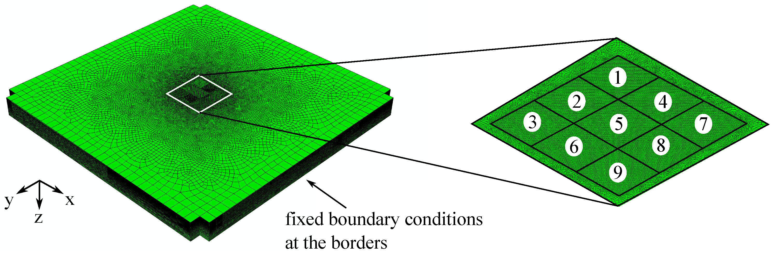
2.2.2. Finite Element Model

An FE model is used to simulate the mechanical shock wave propagation within a target material. The aim of the FE simulation is the prediction of the resulting RS after the LSP treatment, based on the pressure pulse obtained from the global model. The LSP process model follows the set-up presented by Keller et al. [41] and the FE analysis was performed with ABAQUS (Dassault Systèms, Vèlizy-Villacoublay, France). Continuum elements (C3D8R) with an approximate element size of 0.075 × 0.075 × 0.032 mm 3 were used near the laser spot, where the size in depth direction was significantly smaller than parallel to the surface plane. The borders of the FE model were fixed, but the top (target surface) and back surfaces were left unconstrained, simulating free surfaces; see Figure 5. Note that possible reflections of the mechanical stress wave at the back surface were assumed to not affect the resulting RS, as demonstrated in Keller et al. [41]. Laser impacts were simulated as pressure loadings acting locally on the target surface. The time-dependent pressure loading was assumed to be spatially constant, as the experimental spatial laser intensity distribution was almost constant [41].
The shock wave propagation, assumed as a purely mechanical process, leads to extremely high strain rates within the material. Assuming a temperature-independent shock wave propagation, the strain-rate-dependent (reduced) Johnson–Cook model [39] was used:
σ Y = A + B ε P n 1 + C ln ε ˙ P ε ˙ P , 0 ,
where σ Y is the yield stress, ε P the plastic strain and ε ˙ P the plastic strain rate. The material parameter A (yield strength), B (strengthening coefficient) and n (strain hardening exponent) correspond to the behavior at a reference plastic strain rate ε ˙ P , 0 . C describes the rate dependency of the material. The material parameters used in the FE simulations are summarized in Table 2.
The value of the simulated laser impact was limited to a square of 3 × 3 laser pulses to minimize the required computational costs. This is justified by a periodicity assumption, proven by Keller et al. [41], which leads to the fact that the RS of the middle spot (spot 5) are representative of peening a large area, i.e., the peened area of the conducted experiments, except all spots at the edge of the LSP pattern. The sequence of applied pressure pulses is indicated in Figure 5. To be able to compare the experimentally determined and numerically calculated RS, the RS of the simulation were averaged layer-wise in the volume below the middle spot. The indicated scatter of the simulation represents the standard deviation used to calculate the stress average at the respective depth. An explicit solver was used for the pulse phases as well as the relaxation phases of approximately 100 μ s between subsequent pressure pulses, except the last, where an implicit solver was used to calculate the final equilibrium stress state.

2.3. Model Analysis

2.3.1. Sensitivity Study

The set of Equations (1)–(16) was discretized in the time domain with a regular finite difference scheme and solved in Wolfram Mathematica 11.2 (Wolfram Research, Champaign, IL, USA) with the Newton–Raphson method. As initial values for water and metal quantities, the parameters of the unshocked regions were chosen. A breakdown phenomenon [50] was not taken into account in the model, but it was assumed that the plasma already existed at t = 0 and that the initial expansion speeds of the plasma in the water U pw and metal U pm directions were zero. Thus, the initial plasma pressure could be determined from Equations (7) and (8) to P p 0 = 10 5 Pa.
The unknown values are the initial plasma density ρ p 0 and the absorption coefficient A p . Based on the work of Wu and Shin [28], the initial plasma density ρ p 0 is in the range of 0.1 to 10 kg / m 3 for peak laser intensities I max of 1.5 GW / cm 2 (3 J laser pulse) and 2.3 GW / cm 2 (5 J laser pulse). The value of the absorption coefficient A p is assumed to be in the range of 10% [51] to 50% [52]. All initial plasma parameters, including the range of the unknown initial density, are summarized in Table 3.
To investigate the sensitivity of the model regarding the initial plasma density ρ p 0 and absorption coefficient A p , a sensitivity analysis was performed for the case of a 5 J laser pulse without the application of a coating material. The resulting maximum plasma pressure P max is depicted as a function of ρ p 0 for different values of A p in Figure 6. It can be observed that an increase in the initial density leads to a decrease in P max , because the expansion speed of the plasma in the direction of water increases in the model—see Figure 7b—which means a faster increase in the plasma volume instead of a confinement. Increasing A p results in an increase in P max . For initial plasma densities below 0.5 kg / m 3 , the resulting pressure shows unphysical behavior, because the internal plasma energy reaches a singularity in the limit for ρ p 0 0 ; therefore, this region is disregarded from the relevant parameter domain.
The four points (P1, P2, P3, P4) at the borders of the considered parameter space of ρ p 0 and A p —see Figure 6—were chosen in order to study the plasma and the shock wave behavior in the model in detail. Temporal distributions of water and metal parameters for the first 300 ns for these four points are shown in Figure 7 and Figure 8. The results for the metal and water shock region illustrate that a higher initial plasma density results in a faster decrease in the particle and plasma expansion velocities after reaching the maximum value. The particle velocity of water is approximately five times larger than the velocity of metal particles; see Figure 7a,c. The expansion speed of plasma in the direction of water is one order higher than the expansion speed in the direction of metal; see Figure 7b,d.
After the comparison of the plasma expansion speeds U pm and U pw with the particle velocities of metal U m and water U w , respectively, it is obvious that a mass flow into plasma exists; see Figure 8. The application of higher absorption coefficients leads to increased mass flows into plasma at the same initial plasma densities. The major mass flow comes from water, which indicates that the plasma mostly consists of water particles. These results agree with those of [28,30]. However, the existing mass flow from the metal shows that the plasma contains also a significant fraction of metallic particles.
The resulting temporal plasma pressure distributions for the four parameter combinations are depicted in Figure 9. The calculated pressures decrease very slowly after the laser terminates, i.e., after 80 ns ; see Figure 9a. However, taking into account the relaxation process, accounted for by Equation (17), the pressure profiles can be corrected and show reasonable results; see Figure 9b. The pressure profiles have almost identical shapes for different sets of initial parameters, but the maximum values differ in the range of 0.75 to 3.25 GPa . These pressures are over the Hugoniot elastic limit for the considered aluminum alloy, leading to plasticity within the target material, resulting in residual stresses.

2.3.2. Residual Stress Prediction

In the next step, the determined pressure pulses are applied as surface loading in the FE simulations to predict residual stresses in the target material, as described in Section 2.2.2. The resulting RS for the four parameter combinations are depicted in Figure 10a. Depending on the specific pressure profile, the RS distributions show different behavior. The largest pressure P 1 produces compressive RS with a maximum value less than 100 MPa over a depth between 0.5 mm and 1.5 mm . In contrast to this, the lowest pressure P3 causes a shock wave, which does not even exceed the yield stress at a depth of 0.3 mm . An increase in the maximum pressure leads to an increase in the maximum compressive RS, up to a saturated value. After this value is reached, the further increase in the maximum pressure leads more to a shift in the position of the maximum RS together with a slight decrease and a more uniform over-the-depth stress distribution.

2.3.3. Parameter Identification

In this section, the unknown initial plasma density ρ p 0 and the laser absorption coefficient A P in the global model are identified based on fitting of the predicted RS to the experimentally obtained ones. As observed from the comparison of measured and simulated RS, discussed in Section 3.2 and shown in Figure 14b, the required pressure pulse should exhibit a maximum value of approximately 1.5 GPa. It is sufficient to focus merely on the maximum value, because the shape of the simulated pressure pulses is almost identical; see Figure 9. Such a maximum pressure corresponds to a variety of combinations of ρ p 0 and A P ; see Figure 6. Thus, additional data are necessary.
Wu and Shin presented the maximum plasma density ρ pmax dependent on the laser intensity [28], from which ρ pmax 340 kg / m 3 can be identified for the laser intensity of 2.3 GW / cm 2 (5 J laser pulse). Due to this, it is useful to determine the relation between the maximum plasma pressure and the maximum plasma density from the sensitivity analysis for different absorption coefficients A P , as depicted in Figure 10b. This relation allows us to identify A P 17 % for ρ pmax 340 kg / m 3 and a maximum plasma pressure of approximately 1.5 GPa. Based on this result, the initial plasma density can be determined from Figure 6 as ρ p 0 = 2 kg / m 3 . The resulting pressure pulse and RS distribution are shown in Figures 11b and 14b from Section 3.2, respectively.

3. Results and Discussion

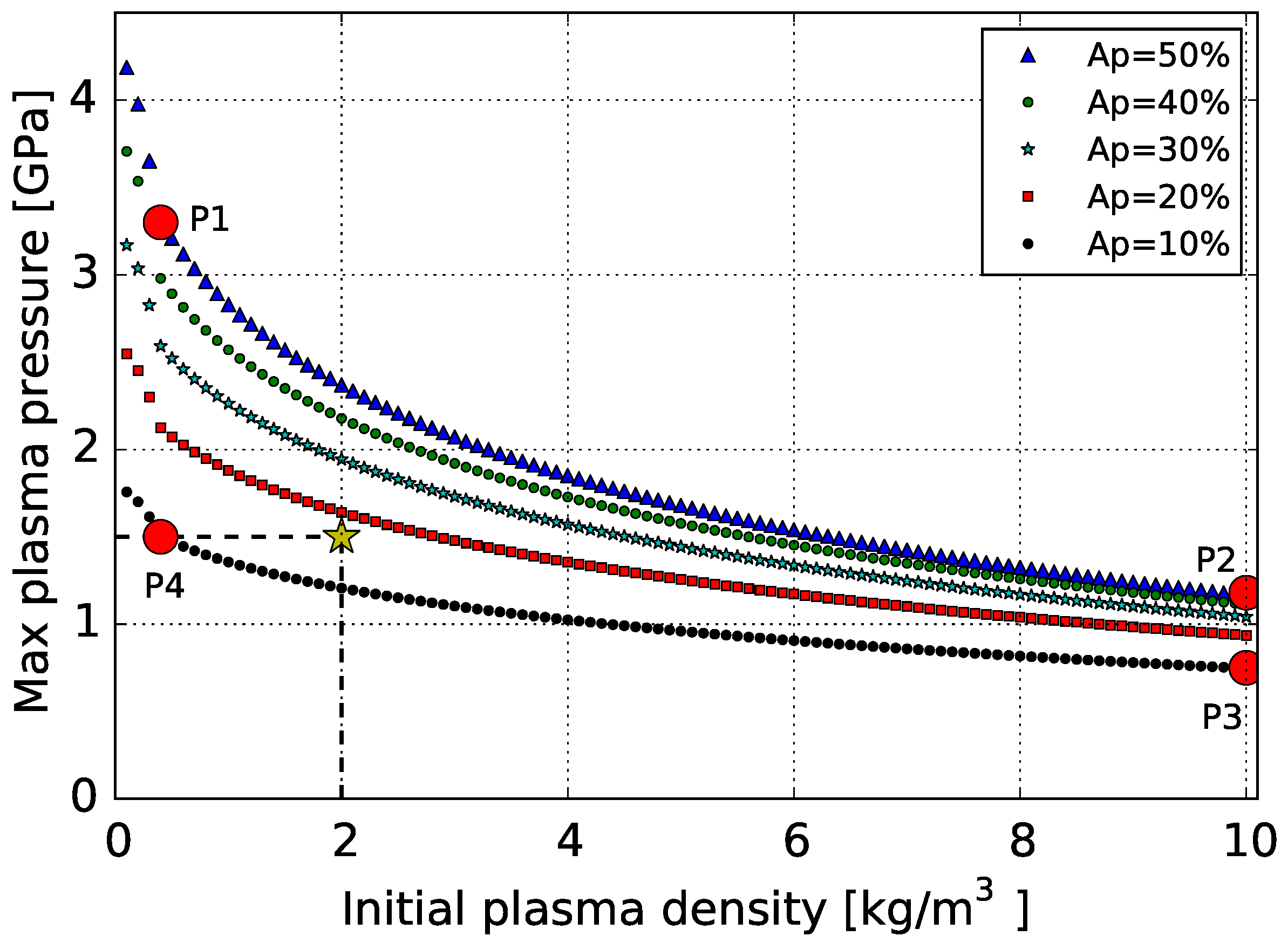
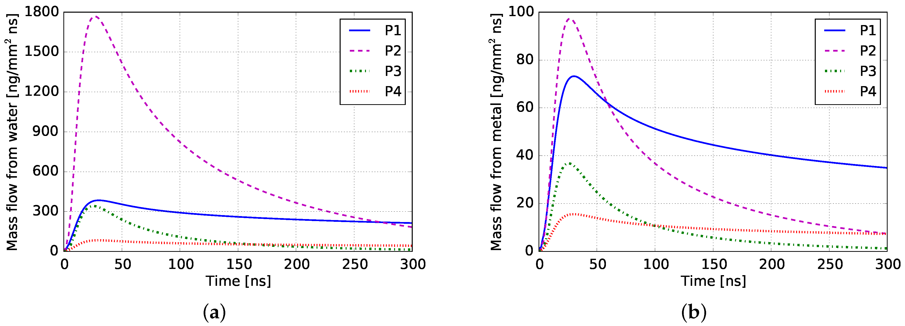
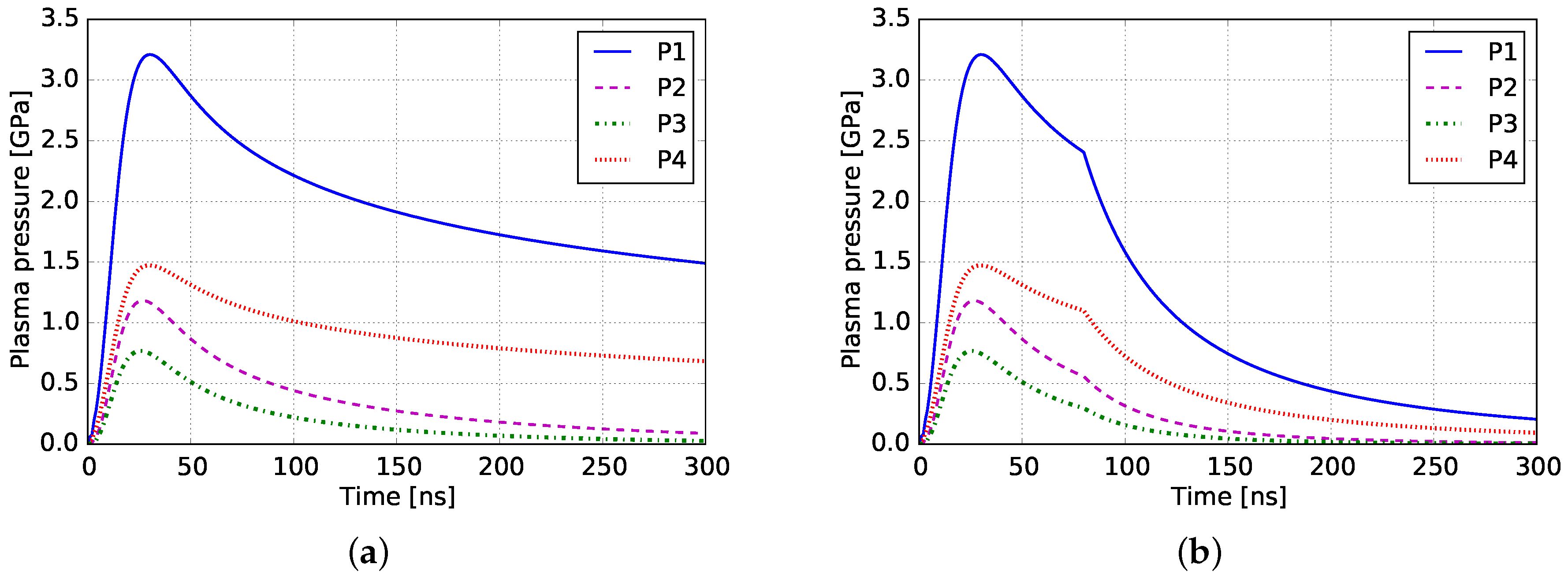
3.1. Pressure Profiles

Based on the identified parameter set at a peak laser intensity of 2.3 GW / cm 2 (5 J laser pulse), further LSP cases, such as 3 J laser pulse energy and different coating materials (aluminum foil and steel foil), are investigated.
Due to the fact that the radiation absorption by plasma does not strongly depend on the laser intensity, when the intensity is lower than 2.3 GW / cm 2 (5 J laser pulse) [27], and considering the fact that the plasma mostly consists of water particles—see Section 2.3.1—the absorption coefficient A P is assumed to remain constant for both 3 J and 5 J laser pulses and the different coating materials used in this study.
For different coating materials, different phase change energies are taken into account in the global model. Lower phase change energies result in higher initial plasma densities for the same laser parameter due to the fact that the initial plasma completely consists of metal particles produced by the material surface ablation. Therefore, the initial plasma density for the ablation of a steel coating is determined to be 3.2 kg / m 3 , as the phase change energy of steel is approximately 1.6 times lower than for aluminum; see Table 1.
The resulting temporal plasma pressure distributions are depicted in Figure 11. Due to the fact that the global model does not distinguish between the ablation of aluminum foil and an aluminum sample without coating, the predicted pressure distributions for these cases are identical. All pressure distributions show similar profiles, where the maximum occurs after the laser intensity peak and the pressure duration is approximately three times longer than the laser pulse duration. This is due to the mass flow from water to plasma, which agrees well with the observations of Zhang et al. [30] and Wu et al. [28]. Furthermore, the increase in the laser pulse energy from 3 J to 5 J results in a ∼25% maximum pressure increase.
Moreover, the usage of a steel foil as a coating material results in a ∼10% maximum pressure decrease in comparison with an aluminum ablative surface. The reason for this is, on one hand, the increased initial plasma density, which results in an increase in the plasma expansion velocity in the direction of water. As described in Section 2.3.1, faster expansion of the plasma—see also Figure 12—indicates less confinement.On the other hand, a significantly reduced mass flow from metal to plasma is observable in Figure 13, which seems to be the major reason for the reduced pressure.

3.2. Residual Stresses

The calculated temporal plasma pressure distributions—see Figure 11—were used in the FE simulations for RS prediction, which were subsequently compared with the experimental results; see Figure 14. Both the simulated and experimental RS profiles agree well for the different investigated cases. A higher pulse energy results in a deeper penetration depth and a slightly higher maximum compressive RS. The usage of foils as ablative coatings allows us to avoid surface-near tensile RS, which are probably induced due to the melting process of the metal surface layer [53]. However, melting phenomena are not taken into account during the FE simulations; this is why the RS predictions deviate from the experimental results near the surface region in the case of LSP without coating.
The simulated RS for 3 J without foil are in good agreement with the experimental RS determination, which demonstrates the applicability of the identified plasma parameter for 5 J laser pulses also in the 3 J case. Experiments show that the application of an aluminum coating leads to a higher maximum compressive stress and indicate a slightly deeper penetration of compressive RS compared to LSP without coating; see Figure 14a,c for 3 J and Figure 14b,d for 5 J. This observation is consistent with the literature [54]. The corresponding simulation result shows some disagreement with the experimental data, probably due to the fact that the global model does not take into account the effect of the interface between the foil and target material (AA2198). In the case of the steel ablative coating, the predicted RS are in good agreement with the experimental results. This shows that the reduced plasma pressure, as depicted in Figure 11, causes a reduced penetration depth and reduced compressive stresses, although the predicted penetration depth is slightly underestimated.
A comparison of measured RS for 5 J pulse energy and 3 J shows a tendency towards unequal σ x x M and σ y y M in cases with a higher laser pulse energy. While this tendency towards a non-equibiaxial RS field agrees with previous work—see, e.g., Kallien et al. [55]—the non-equibiaxial characteristic of this RS field is not very pronounced.
In the case of the steel foil, the maximum compressive stress increases due to an increased pressure pulse caused by a higher laser energy. Comparing the measurements with aluminum foil shows that the maximum compressive stress is slightly decreased and located deeper in the case of 5 J energy. In addition, a higher pulse energy results in a flatter RS distribution.
However, good agreement between the simulated and measured RS patterns indicates that the proposed coupled simulation approach of the global and FE model is applicable to different laser intensities and coating materials to predict RS distributions.

4. Conclusions

Within this study, a two-step model, which includes a global model and following FE simulations, was applied to the LSP of aluminum alloy AA2198-T3 with water confinement. The global model is based on the model proposed by Zhang et al. [30] and deals with the laser–matter interaction, where temporal distributions of physical quantities in metal, water and plasma are identified. The key results—temporal pressure profiles at the material surface—are used in subsequent FE simulations in order to predict the RS state of the target after treatment. The predicted RS distributions were compared with measurement results for different coating materials (aluminum and steel foils) and two laser pulse energies (3 J and 5 J) with a 3 × 3 mm 2 square laser focus in order to validate the proposed simulation scheme.
The nonlinear global model contains two unknown parameters: the initial plasma density and the laser absorption coefficient, which represents the pure laser pulse energy absorption in the plasma. A conducted sensitivity study demonstrates the importance of these unknown plasma parameters, which were identified by fitting the calculated RS to the experimentally determined RS for the laser pulse energy of 5 J. Thereafter, the pure energy absorption of the laser in the plasma was determined to 17 % and the initial plasma density to 2 kg / m 3 in cases with an aluminum ablative surface. Besides this, it was shown that mass flow from water into plasma is a few times higher than from metal. This means that the plasma mostly consists of water particles, which agrees with former results, and that its high mass flow causes the high plasma pressure and broader pressure peak in water confinement cases compared to ablation in vacuum. Due to this, the energy absorption can be assumed constant for different coating layers and small variations in the laser intensity. The effect of different coating layers can be treated by the phase change energy and influences the initial plasma density and the mass flow to plasma. In the case of a steel foil, a value of 3.2 kg / m 3 was estimated, which increases the initial plasma density and thus the expansion velocity in the direction of plasma. This indicates less confinement compared to the results with an aluminum foil. In addition, a reduced mass flow from metal to plasma is determined, which is probably the main reason for the decreased maximum plasma pressure in the model.
The identified temporal plasma pressure distributions for the laser pulse energies of 3 J and 5 J as well as for the conditions with no coating, aluminum and steel coating, were used as surface pressures in subsequent FE simulations to predict RS profiles over depth within the target material. The FE model considers the mechanical shock wave propagation as a purely mechanical process using the strain-rate-dependent (reduced) Johnson–Cook model [39]. The predicted RS profiles were compared with measurements obtained using the incremental hole drilling technique [42] and show good agreement. A higher laser pulse energy (5 J vs. 3 J) results in a deeper penetration depth and a slightly higher maximum compressive RS. The usage of foils as ablative coatings allows the avoidance of surface-near tensile RS. Besides this, it was shown that application of a steel foil causes a decreased maximum plasma pressure in comparison with the aluminium foil case. As a result, reduced compressive stresses and penetration depths were observed when a steel foil was used.
Overall, it is shown that the proposed coupled simulation approach of global and FE model can be used to predict RS distributions using different coating materials and laser intensities. In this approach, the applied global model is a good compromise between simplicity and accuracy, because it allows us to determine time-dependent plasma and shocked regions’ parameters in short simulation times, taking mass flows between metal, plasma and confinement into account.

Author Contributions

Conceptualization, V.P., S.K., B.K. and J.O.; methodology, V.P. and S.K.; software, V.P. and S.K.; formal analysis, V.P.; investigation, V.P. and S.K.; resources, N.K. and J.O.; data curation, V.P. and S.K.; writing—original draft preparation, V.P. and S.K.; writing—review and editing, V.P., S.K., N.K., B.K. and J.O.; visualization, V.P. and S.K.; supervision, N.K., B.K. and J.O.; project administration, N.K., B.K. and J.O. All authors have read and agreed to the published version of the manuscript.

Funding

This research received no external funding.

Institutional Review Board Statement

Not applicable.

Informed Consent Statement

Not applicable.

Data Availability Statement

The data presented in this study are available upon reasonable request from the corresponding authors.

Conflicts of Interest

The authors declare no conflict of interest.

Abbreviations

The following abbreviations are used in this manuscript:
Ayield strength
A p coefficient of laser absorption by the plasma
Bstrengthening coefficient
Γ mass flow
Crate dependency of the material
Dshock wave velocity
Einternal energy
E Y Young’s modulus
E Γ energy exchange through mass flows
E pk kinetic plasma energy
E pt total plasma energy
Flaser focus size
Ilaser intensity
I max peak of laser intensity
Lplasma thickness
Ppressure
P max maximum plasma pressure
Qspecific phase change energy
Sempiric parameters, which connect shock and particle velocities
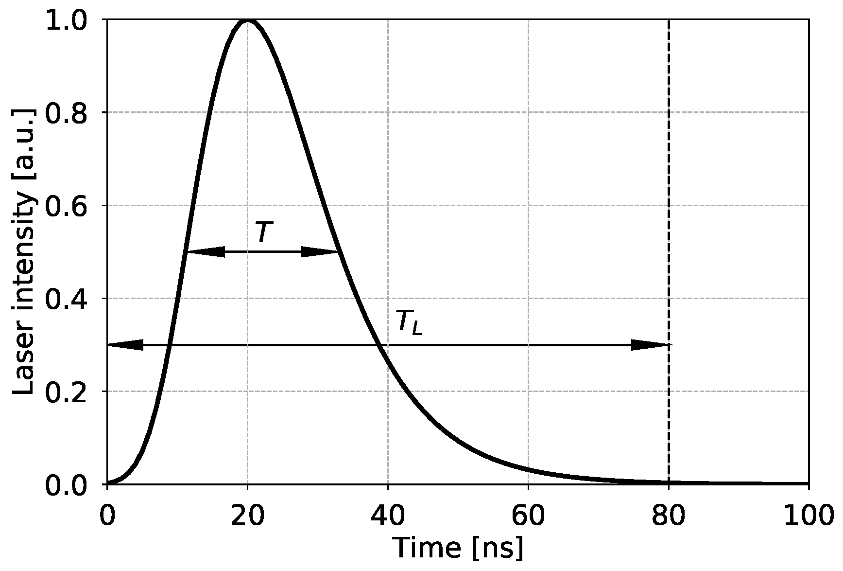
Tlaser pulse FWHM
T L total pulse duration
Uparticles velocity
U pm expansion velocity of plasma in metal direction
U pw expansion velocity of plasma in water direction
U s velocity of sound
W p work done by plasma
γ specific heat ratio
ε P plastic strain
ε ˙ P plastic strain rate
ε ˙ P , 0 reference plastic strain rate
ν Poisson’s ratio
nstrain hardening exponent
ρ mass density
ρ pmax maximum plasma density
σ Y yield stress
σ x x M measured residual stress in xx-direction
σ y y M measured residual stress in yy-direction
σ x x S i m calculated residual stress in xx-direction
σ y y S i m calculated residual stress in yy-direction
ttime
FEfinite element
FWHMfull-width-at-half-maximum
ICFinertial confinement fusion
LSPlaser shock peening
RSresidual stress
Subscript ’m’metal region
Subscript ’0’unshocked region
Subscript ’p’plasma region
Subscript ’w’water region

References

  1. Vilhauer, B.; Bennett, C.R.; Matamoros, A.B.; Rolfe, S.T. Fatigue behavior of welded coverplates treated with Ultrasonic Impact Treatment and bolting. Eng. Struct. 2012, 34, 163–172. [Google Scholar] [CrossRef]
  2. Hatamleh, O. A comprehensive investigation on the effects of laser and shot peening on fatigue crack growth in friction stir welded AA 2195 joints. Int. J. Fatigue 2009, 31, 974–988. [Google Scholar] [CrossRef]
  3. Gujba, A.K.; Medraj, M. Laser Peening Process and Its Impact on Materials Properties in Comparison with Shot Peening and Ultrasonic Impact Peening. Materials 2014, 7, 7925–7974. [Google Scholar] [CrossRef] [PubMed] [Green Version]
  4. Zhu, J.; Jiao, X.; Zhou, C.; Gao, H. Applications of Underwater Laser Peening in Nuclear Power Plant Maintenance. Energy Procedia 2012, 16, 153–158. [Google Scholar] [CrossRef] [Green Version]
  5. Colon, C.; de Andres-Garcia, M.I.; Moreno-Diaz, C.; Alonso-Medina, A.; Porro, J.A.; Angulo, I.; Ocana, J.L. Experimental Determination of Electronic Density and Temperature in Water-Confined Plasmas Generated by Laser Shock Processing. Metals 2019, 9, 808. [Google Scholar] [CrossRef] [Green Version]
  6. Radziejewska, J.; Strzelec, M.; Ostrowski, R.; Sarzyński, A. Experimental investigation of shock wave pressure induced by a ns laser pulse under varying confined regimes. Opt. Laser Eng. 2020, 126, 105913. [Google Scholar] [CrossRef]
  7. Peyre, P.; Fabbro, R.; Berthe, L.; Dubouchet, C. Laser shock processing of materials, physical processes involved and examples of applications. J. Laser Appl. 1996, 8, 135. [Google Scholar] [CrossRef]
  8. Askaryan, G.A.; Moroz, E.M. Pressure on evaporation of matter in a radiation beam. JETP Lett. 1963, 16, 1638. [Google Scholar]
  9. White, R.M. Elastic Wave Generation by Electron Bombardment or Electromagnetic Wave Absorption. J. Appl. Phys. 1963, 34, 2123–2124. [Google Scholar] [CrossRef]
  10. Lindl, J. Development of the indirect-drive approach to inertial confinement fusion and the target physics basis for ignition and gain. Phys. Plasmas 1995, 2, 3933–4024. [Google Scholar] [CrossRef] [Green Version]
  11. Moscicki, T.; Hoffman, J.; Szymanski, Z. Modelling of plasma formation during nanosecond laser ablation. Arch. Mech. 2011, 63, 99–116. [Google Scholar]
  12. Anderholm, N.C. Laser-generated stress waves. Appl. Phys. Lett. 1970, 16, 113–115. [Google Scholar]
  13. O’Keefe, J.D.; Skeen, C.H.; York, C.M. Laser-induced deformation modes in thin metal targets. J. Appl. Phys. 1973, 44, 4622–4626. [Google Scholar] [CrossRef]
  14. Fairand, B.P.; Clauer, A.H.; Jung, R.G.; Wilcox, B.A. Quantitative assessment of laser-induced stress waves generated at confined surfaces. Appl. Phys. Lett. 1974, 25, 431–433. [Google Scholar] [CrossRef]
  15. Warren, A.W.; Guo, Y.B.; Chen, S.C. Massive parallel laser shock peening: Simulation, analysis, and validation. Int. J. Fatigue 2008, 30, 188–197. [Google Scholar] [CrossRef]
  16. Hu, Y.; Yao, Z.; Hu, J. 3-D FEM simulation of laser shock processing. Surf. Coat. Technol. 2006, 201, 1426–1435. [Google Scholar] [CrossRef]
  17. Golabi, S.; Vakil, M.R.; Amirsalari, B. Multi-Objective Optimization of Residual Stress and Cost in Laser Shock Peening Process Using Finite Element Analysis and PSO Algorithm. Lasers Manuf. Mater. Process. 2019, 6, 398–423. [Google Scholar] [CrossRef]
  18. Braisted, W.; Brockman, R. Finite element simulation of laser shock peening. Int. J. Fatigue 1999, 21, 719–724. [Google Scholar] [CrossRef]
  19. Zhai, P.; Dong, Z.; Miao, R.; Deng, X.; Chen, L. Investigation on the laser-induced shock pressure with condensed matter model. J. Appl. Phys. 2015, 54, 056203. [Google Scholar] [CrossRef]
  20. Wei, X.L.; Ling, X. Numerical modeling of residual stress induced by laser shock processing. Appl. Surf. Sci. 2014, 301, 557–563. [Google Scholar] [CrossRef]
  21. Kim, J.H.; Kim, Y.J.; Lee, J.W.; Yoo, S.H. Study on effect of time parameters of laser shock peening on residual stresses using FE simulation. J. Mech. Sci. Technol. 2014, 28, 1803–1810. [Google Scholar] [CrossRef]
  22. Ding, K.; Ye, L. Simulation of multiple laser shock peening of a 35CD4 steel alloy. J. Mater. Process. Technol. 2006, 178, 162–169. [Google Scholar] [CrossRef]
  23. Yang, C.; Hodgson, P.D.; Liu, Q.; Ye, L. Geometrical effects on residual stresses in 7050-T7451 aluminum alloy rods subject to laser shock peening. J. Mater. Process. Technol. 2008, 201, 303–309. [Google Scholar] [CrossRef]
  24. Wang, X.; Xia, W.; Wu, X.; Huang, C. Scaling Law in Laser-Induced Shock Effects of NiTi Shape Memory Alloy. Metals 2018, 8, 174. [Google Scholar] [CrossRef]
  25. Kumar, G.R.; Rajyalakshmi, G. Modelling and multi objective optimization of laser peening process using Taguchi utility concept. IOP Conf. Ser. Mater. Sci. Eng. 2017, 263, 062055. [Google Scholar] [CrossRef]
  26. Jiang, X.; Yu, X.; Deng, X.; Shao, Y.; Peng, P. Investigation on Laser-Induced Shock Pressure with Condensed Matter Model and Experimental Verification. Exp. Tech. 2019, 43, 161–167. [Google Scholar] [CrossRef]
  27. Fabbro, R.; Fournier, J.; Ballard, P.; Devaux, D.; Virmont, J. Physical study of laser-produced plasma in confined geometry. J. Appl. Phys. 1990, 68, 775–784. [Google Scholar] [CrossRef]
  28. Wu, B.; Shin, Y.C. A self-closed thermal model for laser shock peening under the water confinement regime configuration and comparisons to experiments. J. Appl. Phys. 2005, 97, 113517. [Google Scholar] [CrossRef]
  29. Morales, M.; Porro, J.A.; Blasco, M.; Molpeceres, C.; Ocana, J.L. Numerical simulation of plasma dynamics in laser shock processing experiments. Appl. Surf. Sci. 2009, 255, 5181–5185. [Google Scholar] [CrossRef]
  30. Zhang, W.; Yao, Y.L.; Noyan, I.C. Microscale Laser Shock Peening of Thin Films, Part 1: Experiment, Modeling and Simulation. J. Manuf. Sci. Eng. 2004, 126, 10–17. [Google Scholar] [CrossRef]
  31. Pirri, A.N.; Root, R.G. Plasma Energy Transfer to Metal Surfaces Irradiated by Pulsed Lasers. AIAA J. 1978, 16, 1296–1304. [Google Scholar] [CrossRef]
  32. Fortunato, A.; Orazi, L.; Cuccolini, G.; Ascari, A. Laser shock peening and warm laser shock peening: Process modeling and pulse shape influence. Proc. SPIE 1978, 8603, 86030G. [Google Scholar]
  33. Sinha, S. Nanosecond laser ablation of graphite: A thermal model based simulation. J. Laser Appl. 2018, 30, 012008. [Google Scholar] [CrossRef]
  34. MacFarlane, J.J.; Golovkin, I.E.; Woodruff, P.R. HELIOS-CR—A 1-D radiation-magnetohydrodynamics code with inline atomic kinetics modeling. J. Quant. Spectrosc. Radiat. Transf. 2006, 99, 381–397. [Google Scholar] [CrossRef] [Green Version]
  35. Lyon, S.P.; Johnson, J.D. SESAME: The Los Alamos National Laboratory Equation of State Database; Technical Report, LA-UR-92-3407; Los Alamos National Laboratory: Los Alamos, NM, USA, 1992.
  36. Bhamare, S.; Ramakrishnan, G.; Mannava, S.R.; Langer, K.; Vasudevan, V.K.; Qian, D. Simulation-based optimization of laser shock peening process for improved bending fatigue life of Ti–6Al–2Sn–4Zr–2Mo alloy. Surf. Coat. Technol. 2013, 232, 464–474. [Google Scholar] [CrossRef]
  37. Peyre, P.; Fabbro, R.; Merrien, P.; Lieurade, H.P. Laser shock processing of aluminium alloys. Application to high cycle fatigue behaviour. Mater. Sci. Eng. 1996, 210, 102–113. [Google Scholar] [CrossRef]
  38. Amarchinta, H.K.; Grandhi, R.V.; Clauer, A.H.; Langer, K.; Stargel, D.S. Simulation of residual stress induced by a laser peening process through inverse optimization of material models. J. Mater. Process. Technol. 2010, 210, 1997–2006. [Google Scholar] [CrossRef]
  39. Johnson, G.; Cook, W. A Constitutive Model and Data for Metals Subjected to Large Strains, High Strain Rates, and High Temperatures. In Proceedings of the 7th International Symposium on Ballistics, The Hague, The Netherlands, 19–21 April 1983; pp. 541–547. [Google Scholar]
  40. Langer, K.; Olson, S.; Brockman, R.; Braisted, W.; Spradlin, T.; Fitzpatrick, M.E. High Strain-Rate Material Model Validation for Laser Peening Simulation. J. Eng. 2015, 2015, 150–157. [Google Scholar] [CrossRef]
  41. Keller, S.; Chupakhin, S.; Staron, P.; Maawad, E.; Kashaev, N.; Klusemann, B. Experimental and numerical investigation of residual stresses in laser shock peened AA2198. J. Mater. Process. Technol. 2018, 255, 294–307. [Google Scholar] [CrossRef]
  42. Schajer, G.S. Advances in hole-drilling residual stress measurements. Exp. Mech. 2010, 50, 159–168. [Google Scholar] [CrossRef]
  43. Meyers, M. Shock Waves and High-Strain-Rate Phenomena in Metals; Springer: Boston, MA, USA, 1981; pp. 1033–1049. [Google Scholar]
  44. NIST Chemistry WebBook. Available online: https://webbook.nist.gov (accessed on 1 June 2019).
  45. Material Property Data. Available online: http://www.matweb.com (accessed on 1 June 2019).
  46. Liley, P.E. Thermophysical Properties of Fluids. In Mechanical Engineers Handbook: Energy and Power, 3rd ed.; Kutz, M., Ed.; John Wiley & Sons, Ltd.: Hoboken, NJ, USA, 2005; Volume 4, pp. 1–45. [Google Scholar]
  47. Leitner, M.; Leitner, T.; Schmon, A.; Aziz, K.; Pottlacher, G. Thermophysical Properties of Liquid Aluminum. Metall. Mater. Trans. A 2017, 48, 3036–3045. [Google Scholar] [CrossRef] [Green Version]
  48. Simons, G.A. Momentum Transfer to a Surface When Irradiated by a High-Power Laser. AIAA J. 1984, 22, 1275–1280. [Google Scholar] [CrossRef]
  49. Sticchi, M.; Staron, P.; Sano, Y.; Meixer, M.; Klaus, M.; Rebelo-Kornmeier, J.; Huber, N.; Kashaev, N. A parametric study of laser spot size and coverage on the laser shock peening induced residual stress in thin aluminium samples. J. Eng. 2015, 2015, 97–105. [Google Scholar] [CrossRef]
  50. Ready, J.F. Effects of High-Power Laser Radiation; Academic: London, UK, 1971. [Google Scholar]
  51. Mahdavi, M.; Ghazizadeh, S.F. Linear absorption mechanisms in laser plasma interactions. J. Appl. Sci. 2012, 12, 12–21. [Google Scholar] [CrossRef]
  52. Zhang, W.; Yao, Y.L. Modeling and Simulation Improvement in Laser Shock Processing. In Proceedings of the ICALEO 2001 Congress, Jacksonville, FL, USA, 15–18 October 2001; pp. 59–68. [Google Scholar]
  53. Rubio-Gonzalez, C.; Gomez-Rosas, G.; Ocana, J.; Molpeceres, C.; Banderas, A.; Porro, J.; Morales, M. Effect of an absorbent overlay on the residual stress field induced by laser shock processing on aluminum samples. Appl. Surf. Sci. 2006, 252, 6201–6205. [Google Scholar] [CrossRef]
  54. Xu, Y.Y.; Ren, X.D.; Zhang, Y.K.; Zhou, J.Z.; Zhang, X.Q. Coating Influence on Residual Stress in Laser Shock Processing. Key Eng. Mater. 2007, 353–358, 1753–1756. [Google Scholar] [CrossRef]
  55. Kallien, Z.; Keller, S.; Ventzke, V.; Kashaev, N.; Klusemann, B. Effect of laser peening process parameters and sequences on residual stress profiles. Metals 2019, 9, 655. [Google Scholar] [CrossRef] [Green Version]
Figure 1. Schematic of LSP with water confinement.
Metals 12 00107 g001
Figure 2. Schematic of the applied LSP simulation scheme, including the comparison of predicted and experimentally determined RS. The global LSP model yields the plasma pressure. This pressure is used in FE simulations to determine the RS numerically. The predicted RS are compared with measurements to determine unknown plasma parameters for the case of a 5 J energy pulse without coating. Based on this, the global model is adjusted to allow for predictions of RS state at different laser intensities and coating materials.
Metals 12 00107 g002
Figure 3. Non-symmetric temporal profile of the laser pulse used in the current research with FWHM T = 20 ns and the total duration T L = 80 ns .
Metals 12 00107 g003
Figure 4. Schematic of the global LSP model with water curtain. The region of water–metal–plasma interaction is separated into five parts: unshocked and shocked water, unshocked metal, shocked metal coupled with a coating material and a plasma of thickness L. Expansion velocities of plasma in water U pw and metal U pm directions are depicted.
Metals 12 00107 g004
Figure 5. FE model of the LSP process for square laser focus. The borders in x- and y-direction were fixed in all degrees of freedom, where the bottom surface was modeled as a free surface. The laser pulses were modeled as pressure loading, obtained from the global model, in the shown order, corresponding to the applied laser pulse sequence.
Metals 12 00107 g005
Figure 6. Sensitivity analysis of the maximum plasma pressure dependent on initial plasma density ρ p 0 for different absorption coefficients A p . LSP of aluminum with a laser pulse energy of 5 J without coating is simulated. The points P1, P2, P3 and P4 correspond to the borders of the parameter space and represent pairs of values ρ p 0 and A p , which were used within the sensitivity study. The star corresponds to identified simulation parameters based on the comparison to experimental RS results; see Section 2.3.3.
Metals 12 00107 g006
Figure 7. Temporal distributions of particle velocities in water (a) and metal (c); the expansion speed of plasma in water (b) and metal (d) directions for the four points P1–P4; see Figure 6. The particle velocity of water is approximately five times larger than the velocity of metal particles. The expansion speed of plasma in the direction of water is one order higher than the expansion speed in the direction of metal.
Metals 12 00107 g007
Figure 8. Time-dependent mass flows from water region (a) and metal region (b) to plasma for the four border points P1–P4; see Figure 6. The major mass flow from water indicates that the plasma mostly consists of water particles.
Metals 12 00107 g008
Figure 9. Plasma pressure distributions for the four border points P1–P4 defined in Figure 6 without relaxation (a) and with relaxation (b), which happens after laser pulse terminates and results in a pressure drop.
Metals 12 00107 g009
Figure 10. (a) Resulting RS distribution after the application of the four pressure pulses (P1–P4) shown in Figure 9b, which were defined for the four border points P1–P4; see Figure 6. (b) Sensitivity study of the maximum plasma pressure regarding the calculated maximum plasma density ρ pmax at different absorption coefficients A P . The star corresponds to identified simulation parameters based on the comparison to experimental RS; see Section 2.3.3.
Metals 12 00107 g010
Figure 11. Temporal pressure distributions for the cases with aluminum ablative surface (solid black line) and with steel foil as a coating material (dashed-dotted red line) in comparison with laser intensity profiles (dashed blue line) for laser pulse energy of 3 J (a) and 5 J (b).
Metals 12 00107 g011
Figure 12. Temporal distribution of the expansion speed of plasma in water direction for the cases with aluminum ablative surface (solid black line) and with steel foil as a coating material (red line) for laser pulse energy of 3 (a) and 5 J (b).
Metals 12 00107 g012
Figure 13. Time-dependent mass flows from metal to plasma for the cases with aluminum ablative surface (solid black line) and with steel foil as a coating material (red line) for laser pulse energy of 3 (a) and 5 J (b).
Metals 12 00107 g013
Figure 14. Comparison between calculated ( σ x x S i m = σ y y S i m ) and experimentally determined ( σ x x M , σ y y M ) RS in AA2198-T3 after LSP treatment for different laser pulse energies and coating materials. (a) 3 J pulse energy, no coating. (b) 5 J pulse energy, no coating. (c) 3 J pulse energy, aluminum foil. (d) 5 J pulse energy, aluminum foil. (e) 3 J pulse energy, steel foil. (f) 5 J pulse energy, steel foil.
Metals 12 00107 g014
Table 1. Material parameters employed, assuming pressure of unshocked regions P 0 of 10 5 Pa for all materials.
ParameterWaterAluminumSteel
Density ρ 0 , kg / m 3 100028007900
Sound velocity U s  [43], m/s23935328-
Coefficient S [43]1.3331.338-
Specific phase change energy Q [44,45,46,47], MJ / kg ≈3≈15≈9
Table 2. Material parameters of AA2198-T3, taken from [41,49].
ParameterAA2198-T3
Young’s modulus E Y , GPa78
Poisson’s ratio ν 0.33
Quasi-static yield strength A, MPa310
Strengthening coefficient B, MPa1177
Strain hardening exponent n0.894
Reference plastic strain rate ε ˙ P , 0 , s 1 1.8 × 10 4
Dynamic strain hardening coefficient C0.01
Table 3. Initial parameter value ranges for the plasma quantities used in the sensitivity study.
ParameterInitial Value
Expansion velocities U pw and U pm , m/s0
Plasma density ρ p 0 , kg/m 3 0.1–10
Plasma pressure P p 0 , Pa 10 5
Absorption coefficient A p , % 10–50
Publisher’s Note: MDPI stays neutral with regard to jurisdictional claims in published maps and institutional affiliations.

