Abstract
Traditional processing technology is not suitable for the requirements of advanced manufacturing due to the disadvantages of large repeated experiments, high cost, and low economic effect. As the latest additive technology, 3D printing technology has to deal with many issues such as process parameters and nonlinear mathematical models. A three-layer backpropagation (BP) artificial neural network with a Lavenberg–Marquardt algorithm was established to train the network and predict orthogonal experimental data. Additionally, the best combination of parameters of material deformations were predicted and verified by experiments. The results show that the predicted value obtained by the BP model is in good agreement with the experimental value curve, with a small relative error and a correlation coefficient of 0.99985. Moreover, the deformation errors of the printed model are not more than 3%. The incorporation of the BP neural network algorithm into the 3D printing process can, therefore, help cope with related problems, which is a future trend.
1. Introduction
As one of the representative technologies of the four industrial revolutions, 3D printing technology has drawn increasing attention from the industrial sector and the investor community [1,2,3]. 3D printing technology, going by the name of “additive manufacturing” in academic terms, is also known as additive manufacturing or incremental manufacturing. According to the definition published by the 3D Printing Technical Committee (F42 Committee) established by the American Society for Testing and Materials (ASTM) in 2009 [4], 3D printing, based on 3D Computer Aided Design (CAD) model data, is a way of manufacturing by adding materials layer by layer, which is diametrically opposed to traditional material processing methods. It adopts a manufacturing method of directly manufacturing a three-dimensional physical solid model that is completely consistent with the corresponding mathematical model [5]. The content of 3D printing technology covers all printing processes, technologies, equipment categories, and applications related to “rapid prototyping” at the front end of the product life cycle and “rapid manufacturing” at the full production cycle [6]. The technologies involved in 3D printing include the integration of CAD modeling, measurement, interface software, numerical control, precision machinery, lasers, materials, and other disciplines [7]. At present, the materials that have been developed mainly include plastics [8], resins [9], and metals [10]. However, for 3D printing technology to be applied in more fields, it is necessary to develop more printable materials. According to the characteristics of the materials, the relationship between processing, structure, and materials needs to be delved into in depth. Besides, efforts should be made to develop quality test procedures and methods, establish normative standards for material performance data, etc. [11]. Compared with traditional processes, the main advantages of additive manufacturing are (1) rapid manufacturing of complex structures [12]; (2) support personalized customization [13]; and (3) precise manufacturing processes [14]. Therefore, 3D printing technology is widely applied in stereo lithography apparatus, polymer, three-dimensional printing, gluing, and fused deposition modeling [15,16,17].
However, for the printing process, there is more than one printing parameter, such as printing speed (10–80 mm/s), printing temperature (100–300 °C), filling density (10–70%), scanning speed (10–70 mm/s), and initial layer thickness (0.1–0.5 mm), and it is necessary to continuously adjust and optimize the process parameters according to the expected plan. Following that, a large number of repeated experiments need to be carried out, which will result in the waste of printing materials and time costs, going against the goal of sustainable development. To handle the above-mentioned difficulties, the use of artificial neural networks (ANN) [18,19] to guide the experiment is expected to obtain excellent experimental parameters for experimental verification. The backpropagation (BP) neural network, one of the methods of the artificial neural network, plays a significant role in dealing with many problems that cannot be clearly defined in the mathematical model [20,21]. The test samples set were trained and adjusted by the self-learning function. The powerful mapping ability of BP neural network was then used to store the learned information in the weight under the self-organization performance through the learning of the samples [22]. The trained BP neural network displayed a strong, non-linear mapping ability with unconstrained output samples set when the training samples were input again [23]. The BP neural network, when applied to solve real-life problems, can bring huge benefits to people [24,25,26,27]. To sum up, it is found that there are few studies on the BP neural network optimization of 3D printing parameters, and there is also a lack of theoretical support. Therefore, combining BP with 3D printing technology to optimize the predicted deformation is a strong potential design concept, which opens up a new way for the combination of artificial intelligence and 3D printing technology.
Based on the analysis of the influence of the weight of the 3D printing material on the deformation amount, this paper employs the BP neural network to optimize the process parameters in the printing process by the orthogonal experiment and finally obtains the process parameter combination with the smallest amount of material deformation. Additionally, the 3D printing model prepared with the best combination of process parameters delivers the best functions.
2. Experimental Method
The experiment used a 3D printer assembled by parts produced by Zhongshan Rainbow Printer Consumables Co., Ltd. (Zhongshan, China), as shown in Figure 1. The printing material is polylactic acid (PLA) material with primary color 1.75 mm, produced by Dongguan Dezhijian Plastic Electronics Co., Ltd. (Dongguan, China).
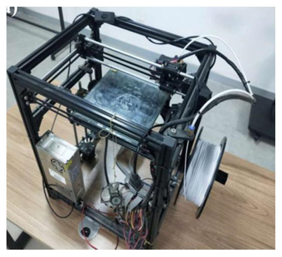
Figure 1.
PLA-3D assembled printer.
2.1. Design of the Print Model
Material deposition characteristics are related to printing speed, filling density, printing temperature, printing layer thickness, and other parameters. In this experiment, the STL format was exported after UG modeling [28], and the data were imported into a 3D printer for model printing after processed with Cura slicing software (version 15.06, Ultimaker, Utrecht, The Netherlands), as shown in Figure 2.
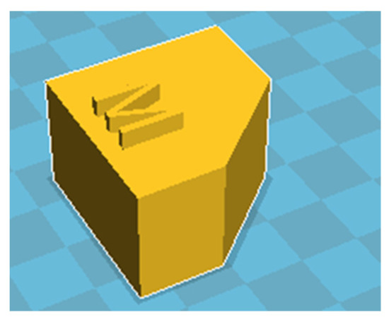
Figure 2.
The 3D printer for mode.
2.2. Design of the Orthogonal Test
The orthogonal experiment was designed to reasonably classify the test data and factors, put them into a pre-set, neatly arranged table and conduct overall design, comprehensive comparison, and statistical analysis [29,30]. Under experimental conditions, the optimal process parameters are found through the comparison of the test results of each group and range analysis, and then the process products with better performance are obtained [31].
In this experiment, the amount of deformation S (mm/mm) of the printed material is used as an inspection index, while printing speed A (mm/s), printing temperature T (°C), filling density W (%), and initial layer thickness D (mm) are the same as the variable factors, as shown in Table 1. Moreover, the L9 (34) orthogonal experimental [32] results are shown in Table 2. Levels 1, 2, and 3, respectively, indicate the influence of each factor (In terms of column), and the 9 test results are divided into 3 groups corresponding to each level of each factor (column). Moreover, we consider the average value of the deformation in the X/Y/Z direction. The calculation process of the deformation amount is as follows: the set length is a1 (mm), the actual printing length is b1 (mm), and the deformation amount is A = |b1 − a1|/a1. In the Y direction, the calculation process of the deformation amount is as follows: the set length is a2 (mm), the actual printing length is b2 (mm), and the deformation amount is B = |b2 − a2|/a2. In the Z direction, the calculation process of the deformation amount is as follows: the set length is a3 (mm), the actual printing length is b3 (mm), and the deformation amount is B = |b3 − a3|/a3. The average value of the deformation is S = (A + B + C)/3 (mm/mm).

Table 1.
The levels and factors of the orthogonal test.
Table 2.
Results of the orthogonal test.
According to the principle of orthogonal experiment, three levels of factors have three influencing values. For example, the A (mm/s) factor can be decomposed into test indicators A1, A2, and A3. As shown in Table 1, tests 1, 2, and 3 are determined by the test indicator A1; tests 4, 5, and 6 are determined by the test indicator A2; and tests 7, 8, and 9 are determined by the test indicator A3. The three index values K1, K2, and K3 of factor A (mm/s) can be obtained by calculation, which are 0.42, 0.41, and 0.66, respectively. The experimental indicators T, W, and D can also be calculated by the above theory, as shown in Table 3.
Table 3.
Range analysis of orthogonal test results.
If the influence of the factor on the index of the orthogonal test is 0, then Kj values (j = 1, 2 and 3) should be equal [33]. Calculations in Table 3 indicate that the values of Kj are different, and the result of the orthogonal test changes with the level of the factor. Therefore, based on the relative value of Kj, the influence of level factor Aj (j = 1, 2, and 3) on the index of orthogonal test can be judged. The verification index of the orthogonal experiment is the amount of deformation. The smaller the amount of deformation change, the better the performance. For example, as K2 < K1 < K3 in factor A (mm/s), K2 is the optimal factor level of factor A. Similarly, it can be calculated that T3, W2, and D1 are the optimal levels of factors T, W, and D, respectively. From the analysis on the range Rj value (Rj = max{} − min{}) [32], it can be seen that factor T has the greatest influence, followed by factor A and factor W, and the smallest is factor D, that is, R1T > R1A > R1W > R1D.
To figure out the accuracy of the orthogonal test, an analysis of variance is carried out [34]. The analysis of variance can analyze the size of the test error and thereby test accuracy. It can not only present the order of the influence of each factor and the interaction on the test index but also identify which factors have significant effects and which ones are not significant. For significant factors, the optimal level is selected and strictly controlled in the experiment; for insignificant ones, the optimal level can be determined according to specific circumstances. The calculation formula is as follows [35]:
where n is the orthogonal test number; s is the number of test repetitions; is the t-th retest of the i-th test; and T is the sum of all test data. The degree of freedom is , and m is the number of factor levels.
It can be seen from Table 4 that the effects of the four factors are distinct, and the significance level is T > A > W > D. Through the comprehensive analysis on the range and variance of the orthogonal test, it can be concluded that the process conditions that affect the deformation S are better: A2T3W2D1. Since the process did not appear in the orthogonal test, the test needs to be verified.
Table 4.
Analysis of variance on amount of deformation S (mm/mm).
2.3. Design of the BP Neural Network
According to the experimental conditions, a simple three layer BP neural network model consisting of input layer, hidden layer, and output layer was designed, as shown in Figure 3. The number of hidden layer nodes has a greater influence on the accuracy of the network. The number of hidden layer nodes can be calculated as follows [36]:
where m is the number of output neurons, n is the number of input neurons, and a is the constant values ranging from 1 to 10. The fastest convergence rate and higher-precision algorithm, Lavenberg–Marquardt (LM), which comprises the Gauss–Newton and the Steepest Descent method of algorithm [37,38], was adopted. The LM algorithm is a network training function that updates weight and bias values [39]. The relative error obtained from this algorithm is smaller than any other algorithm.
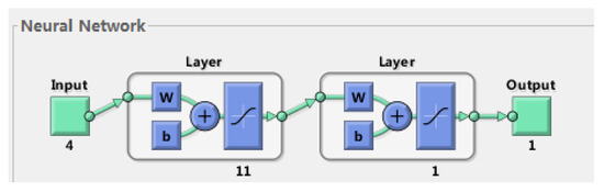
Figure 3.
Schematic description of BP neural network.
The input sample is 4, a figure constructed before the network training according to Table 2 (The orthogonal test data). Then Formula (3) was used to normalize the data, resulting in the value converges between 0 and 1, as shown in Table 5. Similarly, the actual predicted output value of the network can be obtained after the network output value is denormalized by Formula (4).
where is the standardized data, is the experimental data or the data after de-standard processing; and and are the minimum and maximum values of the experiment, respectively.
Table 5.
The normalized data.
The setting of the parameters of the BP neural network is as follows: the neuron function uses tansig (S-tangent function), the output layer neuron function uses purelin, the training function uses trainlm, the learning rate is set to 0.05, and the expected error is 0.001. The normalization function uses premnmx to achieve the result between 0 and 1. After training and simulation [40], the data are denormalized (postmnmx) [41].
3. Results and Discussion
Figure 4 displays the error changes of the BP neural network for corrosion potential and wear rate during training. Figure 4 is the MSE change trend graph during BP neural network training. It can be seen that the network converges to the expected value after a limited number of steps. Therefore, in the 3D printing process, the process effect obtained by different process parameters can be predicted by the established BP neural network mathematical model.
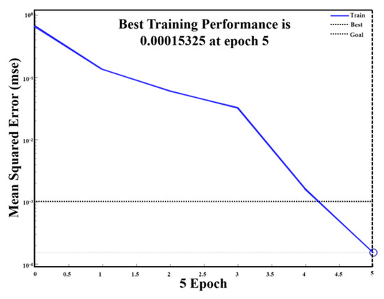
Figure 4.
Error changes of the BP networks based on deformation S amid the training process.
Based on the experimental data in Table 2, the BP neural network model was trained. The experimental values and fitting values are shown in Table 6.
Table 6.
Comparison of experimental and fitting values of deformation in the BP neural network model.
Figure 5 shows that the fitting value of the BP neural network model is highly consistent with the experimental value, and the correlation coefficient is 0.99985. Therefore, the BP neural network model established in the 3D printing process can predict the combined parameters of the smallest deformation [42].
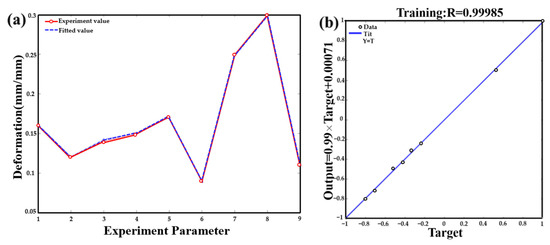
Figure 5.
(a) Comparison of fitting data with experimental data; (b) The curve fitting.
According to the orthogonal experiment, all the combinations of technological level parameters are constructed, that is, 84 combinations. Input these combinations into the BP neural network model established previously for predictive analysis, and the results are shown in Figure 6.
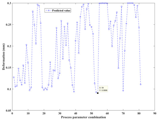
Figure 6.
The optimization combination forecast trend graph.
It can be found that the predicted values are quite close to experimental values. The smallest amount of deformation is 0.0906, which corresponds to the 54th set of parameter combinations, which is A2T3W3D3 (A = 45 mm/s, T = 220 °C, W = 30%, and D = 0.3 mm).
Based on the optimization results of the BP neural network, the parameters A2T3W3D3 are used for corresponding experimental verification. The printed model diagram is shown in Figure 7a. Meanwhile, Figure 7b shows that the physical model printed under the optimization parameters (A2T3W3D3) has a small amount of deformation. Therefore, the BP neural network model plays a guiding role in the 3D printing process, effectively saving time and cost. Moreover, for further verifying the results of deformation, the nine deformation values in the ears, head, and limbs of the model were measured, as shown in Table 7.
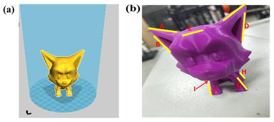
Figure 7.
(a) Print model diagram; (b) physical model diagram.
Table 7.
Comparison of the set values and measured values of printed model.
Through the analysis of the set and measured values of the nine parts (A–I, as marked in yellow solid line in Figure 7b), it can be seen that the deformation error value of the nine parts is less than 5%. It can be seen that it is feasible and reasonable to guide the 3D printing entity construction by using BP neural network to predict parameters.
4. Conclusions
In this manuscript, 3D printing technology, the BP neural network, and the orthogonal experiment are combined to build a model that can be used to predict the deformation of PLA materials in 3D printing technology. Compared with the traditional processing technology, this technology has obvious advantages. Through BP model construction, orthogonal data training, and print parameter optimization, the deformation is verified and predicted. Further, backed up by the principle of the orthogonal experiment, the main factors that affect deformation are obtained as follows: T (°C) > A (mm/s) > W (%) > D (mm). The constructed BP neural network structure delivers good reliability in learning training, simulation test, and numerical prediction. The optimal process parameters are A = 45 mm/s, T = 220 °C, W = 30%, and D = 0.3 mm, and the smallest amount of deformation is 0.0906 mm/mm. The predicted value obtained by the BP model is in good agreement with the experimental value curve, with a small relative error (the maximum value does not exceed 0.1%) and a correlation coefficient of 0.99985. Therefore, this research provides a new approach for studying the application of BP neural network in 3D printing.
Author Contributions
Conceptualization, Y.L.; methodology, Y.L. and W.T.; validation, Y.L. and W.T.; formal analysis, Y.L.; investigation, W.T.; resources, F.D.; writing—original draft preparation, Y.L.; writing—review and editing, Y.L.; project administration, W.T.; and funding acquisition, W.T. All authors have read and agreed to the published version of the manuscript.
Funding
This research is funded by the Special Scientific Research Project of Shaanxi Provincial Department of Education (16JK2219).
Data Availability Statement
The data used to support the findings of this study are available from the corresponding author upon request.
Conflicts of Interest
No conflict of interest exits in the submission of this manuscript, and we have reviewed the final version of the manuscript and approve it for publication. I would like to declare on behalf of my co-authors that the work described was original research that has not been published previously and is not under consideration for publication elsewhere, in whole or in part. All the authors listed have approved the manuscript that is enclosed.
References
- Jaksic, N.I.; Desai, P.D. Characterization of 3D-printed capacitors created by fused filament fabrication using electrically-conductive filament. Procedia Manuf. 2019, 38, 33–41. [Google Scholar] [CrossRef]
- Allen, M.; Chen, W.; Wang, C. 3D printing standards and verification services. Appl. Innov. Rev. 2016, 2, 34–44. [Google Scholar]
- Gopinathan, J.; Noh, I. Recent trends in bioinks for 3D printing. Biomater. Res. 2018, 22, 1–15. [Google Scholar] [CrossRef] [PubMed]
- Monzón, M.D.; Ortega, Z.; Martínez, A.; Ortega, F. Standardization in additive manufacturing: Activities carried out by international organizations and projects. Int. J. Adv. Manuf. Technol. 2015, 76, 1111–1121. [Google Scholar] [CrossRef]
- Bak, D. Rapid prototyping or rapid production? 3D printing processes move industry towards the latter. Assem. Autom. 2003, 23, 340–345. [Google Scholar] [CrossRef]
- Starosolski, Z.A.; Kan, J.H.; Rosenfeld, S.D.; Krishnamurthy, R.; Annapragada, A. Application of 3-D printing (rapid prototyping) for creating physical models of pediatric orthopedic disorders. Pediatr. Radiol. 2013, 44, 216–221. [Google Scholar] [CrossRef]
- Junk, S.; Kuen, C. Review of open source and freeware CAD systems for use with 3D-printing. Procedia CIRP 2016, 50, 430–435. [Google Scholar] [CrossRef]
- Gaikwad, V.; Ghose, A.; Cholake, S.; Rawal, A.; Iwato, M.; Sahajwalla, V. Transformation of E-waste plastics into sustainable filaments for 3D printing. ACS Sustain. Chem. Eng. 2018, 6, 14432–14440. [Google Scholar] [CrossRef]
- Sutton, J.T.; Rajan, K.; Harper, D.P.; Chmely, S.C. Lignin-containing photoactive resins for 3D printing by stereolithography. ACS Appl. Mater. Interfaces 2018, 10, 36456–36463. [Google Scholar] [CrossRef]
- Park, J.-M.; Ahn, J.-S.; Cha, H.-S.; Lee, J.-H. Wear resistance of 3D printing resin material opposing zirconia and metal antagonists. Materials 2018, 11, 1043. [Google Scholar] [CrossRef]
- Rayna, T.; Striukova, L. From rapid prototyping to home fabrication: How 3D printing is changing business model innovation. Technol. Forecast. Soc. Chang. 2016, 102, 214–224. [Google Scholar] [CrossRef]
- Dudek, P. FDM 3D printing technology in manufacturing composite elements. Arch. Met. Mater. 2013, 58, 1415–1418. [Google Scholar] [CrossRef]
- Lee, J.Y.; Tan, W.S.; An, J.; Chua, C.K.; Tang, C.Y.; Fane, A.G.; Chong, T.H. The potential to enhance membrane module design with 3D printing technology. J. Membr. Sci. 2016, 499, 480–490. [Google Scholar] [CrossRef]
- Shahrubudin, N.; Lee, T.C.; Ramlan, R. An overview on 3D printing technology: Technological, materials, and applications. Procedia Manuf. 2019, 35, 1286–1296. [Google Scholar] [CrossRef]
- Juskova, P.; Ollitrault, A.; Serra, M.; Viovy, J.-L.; Malaquin, L. Resolution improvement of 3D stereo-lithography through the direct laser trajectory programming: Application to microfluidic deterministic lateral displacement device. Anal. Chim. Acta 2018, 1000, 239–247. [Google Scholar] [CrossRef]
- Kechagias, J.; Stavropoulos, P.; Koutsomichalis, A.; Ntintakis, I.; Vaxevanidis, N. Dimensional accuracy optimization of prototypes produced by polyJet direct 3D printing technology. Adv. Eng. Mech. Mater. 2014, 978, 61–65. [Google Scholar]
- Liu, Z.; Wang, Y.; Wu, B.; Cui, C.; Guo, Y.; Yan, C. A critical review of fused deposition modeling 3D printing technology in manufacturing polylactic acid parts. Int. J. Adv. Manuf. Technol. 2019, 102, 2877–2889. [Google Scholar] [CrossRef]
- Simionato, G.; Hinkelmann, K.; Chachanidze, R.; Bianchi, P.; Fermo, E.; van Wijk, R.; Leonetti, M.; Wagner, C.; Kaestner, L.; Quint, S. Red blood cell phenotyping from 3D confocal images using artificial neural networks. PLoS Comput. Biol. 2021, 17, 1008934. [Google Scholar] [CrossRef]
- Masi, F.; Stefanou, I.; Vannucci, P.; Maffi-Berthier, V. Thermodynamics-based Artificial Neural Networks for constitutive modeling. J. Mech. Phys. Solids 2020, 147, 104277. [Google Scholar] [CrossRef]
- Ding, S.; Su, C.; Yu, J. An optimizing BP neural network algorithm based on genetic algorithm. Artif. Intell. Rev. 2011, 36, 153–162. [Google Scholar] [CrossRef]
- Zhao, Z.; Xin, H.; Ren, Y.; Guo, X. Application and comparison of BP neural network algorithm in MATLAB. In Proceedings of the 2010 International Conference on Measuring Technology and Mechatronics Automation, Changsha, China, 13–14 March 2010; pp. 590–593. [Google Scholar]
- Ding, S.; Jia, W.; Su, C.; Liu, X.; Chen, J. An improved BP neural network algorithm based on factor analysis. J. Converg. Inf. Technol. 2010, 5, 103–108. [Google Scholar]
- Liu, L.; Chen, J.; Xu, L. Realization and application research of BP neural network based on MATLAB. In Proceedings of the 2008 International Seminar on Future BioMedical Information Engineering, Wuhan, China, 18 December 2008; pp. 130–133. [Google Scholar]
- Panahizadeh, V.; Ghasemi, A.H.; Asl, Y.D.; Davoudi, M. Optimization of LB-PBF process parameters to achieve best relative density and surface roughness for Ti6Al4V samples: Using NSGA-II algorithm. Rapid Prototyp. J. 2022. ahead-of-print. [Google Scholar] [CrossRef]
- Cheng, W.; Fuh, J.Y.H.; Nee, A.Y.C.; Wong, Y.S.; Loh, H.T.; Miyazawa, T. Multi-objective optimization of part-building orientation in stereolithography. Rapid Prototyp. J. 1995, 1, 12–23. [Google Scholar] [CrossRef]
- Cheng, L.; Zhang, P.; Biyikli, E.; Bai, J.; Robbins, J.; To, A. Efficient design optimization of variable-density cellular structures for additive manufacturing: Theory and experimental validation. Rapid Prototyp. J. 2017, 23, 660–677. [Google Scholar] [CrossRef]
- Chen, H.; Zhao, Y.F. Process parameters optimization for improving surface quality and manufacturing accuracy of binder jetting additive manufacturing process. Rapid Prototyp. J. 2016, 22, 527–538. [Google Scholar] [CrossRef]
- Modi, Y.K.; Sanadhya, S. Design and additive manufacturing of patient-specific cranial and pelvic bone implants from computed tomography data. J. Braz. Soc. Mech. Sci. Eng. 2018, 40, 503. [Google Scholar] [CrossRef]
- Ruijiang, L.; Yewang, Z.; Chongwei, W.; Tang, J. Study on the design and analysis methods of orthogonal experiment. Exp. Technol. Manag. 2010, 9, 52–55. [Google Scholar]
- Feng, Z.K.; Niu, W.J.; Cheng, C.T.; Liao, S.L. Hydropower system operation optimization by discrete differential dynamic programming based on orthogonal experiment design. Energy 2017, 126, 720–732. [Google Scholar] [CrossRef]
- Morelli, E.; DeLoach, R. Wind tunnel database development using modern experiment design and multivariate orthogonal functions. In Proceedings of the 41st Aerospace Sciences Meeting and Exhibit, Reno, Nevada, 6–9 January 2003; p. 653. [Google Scholar]
- Sun, W.; Tian, M.; Zhang, P.; Wei, H.; Hou, G.; Wang, Y. Optimization of plating processing, microstructure and properties of Ni–TiC coatings based on BP artificial neural networks. Trans. Indian Inst. Met. 2016, 69, 1501–1511. [Google Scholar] [CrossRef]
- Dong, R.H.; Xiao, B.H.; Fang, Y.S. The theoretical analysis of orthogonal test designs. J. Anhui Inst. Archit. 2004, 6, 29. [Google Scholar]
- Nelder, J.A. The analysis of randomized experiments with orthogonal block structure. II. Treatment structure and the general analysis of variance. Proc. R. Soc. Lond. Ser. A Math. Phys. Sci. 1965, 283, 163–178. [Google Scholar]
- Li, Y.; She, L.; Wen, L.; Zhang, Q. Sensitivity analysis of drilling parameters in rock rotary drilling process based on orthogonal test method. Eng. Geol. 2020, 270, 105576. [Google Scholar] [CrossRef]
- Zhang, W.F.; Zhu, D.; Zeng, Y.B. Study of optimizing process parameters about Ni-SiC composite electrodeposition based on BP neural network. J. Funct. Mater. 2004, 35, 383–384. [Google Scholar]
- Ning, Y.; Liu, Y.; Zhang, H.; Ji, Q. Comparison of different BP neural network models for short-term load forecasting. In Proceedings of the 2010 IEEE International Conference on Intelligent Computing and Intelligent Systems, Xiamen, China, 29–31 October 2010; pp. 435–438. [Google Scholar]
- Saini, L.; Soni, M. Artificial neural network based peak load forecasting using Levenberg–Marquardt and quasi-Newton methods. IEEE Proc. Gener. Transm. Distrib. 2020, 149, 578–584. [Google Scholar] [CrossRef]
- Selvakumar, N.; Radha, P.; Narayanasamy, R.; Davidson, M.J. Prediction of deformation characteristics of sintered aluminium preforms using neural networks. Model. Simul. Mater. Sci. Eng. 2004, 12, 611. [Google Scholar] [CrossRef]
- Liu, X.S.; Deng, Z.; Wang, T.L. Real estate appraisal system based on GIS and BP neural network. Trans. Nonferrous Met. Soc. China 2011, 21, s626–s630. [Google Scholar] [CrossRef]
- Wan, Y.; Wu, J.; Chu, R.; Miao, Z.; Fan, L.; Bai, L.; Meng, X. Prediction of BP neural network and preliminary application for suppression of low-temperature oxidation of coal stockpiles by pulverized coal covering. Can. J. Chem. Eng. 2020, 98, 2587–2598. [Google Scholar] [CrossRef]
- Shenglong, W.; Tonghui, S. The application on the forecast of steam turbine exhaust wetness fraction with GA BP neural network. World Autom. Congr. 2012, 2012, 1–4. [Google Scholar]


Publisher’s Note: MDPI stays neutral with regard to jurisdictional claims in published maps and institutional affiliations. |
© 2022 by the authors. Licensee MDPI, Basel, Switzerland. This article is an open access article distributed under the terms and conditions of the Creative Commons Attribution (CC BY) license (https://creativecommons.org/licenses/by/4.0/).