Modelling of Single-Gas Adsorption Isotherms

Abstract

The present paper reviews and analyses different models that could be used to describe the adsorption equilibrium of pure gases. The adsorption equilibrium of hydrogen, nitrogen and methane is characterised and modelled. Several thermodynamic conceptions have been selected and tested for the calculation of physico-chemical parameters. The model of Dubinin has been selected to estimate the pseudo-saturation vapour pressure. The best results for the molar volume of the adsorbate have been obtained by using Do’s equation. Eight models, namely Langmuir, Freundlich, Sips, Toth, Jovanovic, UNILAN, OBMR and Potential Theory, describing the adsorption equilibrium of pure gases, have been tested and compared with experimental data obtained from the literature at three different temperatures (283 K, 298 K and 313 K). In order to determine the best fit, the correlation coefficient and the standard errors for each parameter have been used to evaluate the data. All the models used in this study, except for Freundlich’s equation in the case of nitrogen or methane adsorption, are in good agreement between experiment and modelling for the adsorption isotherms.

1. Introduction

The gas physisorption phenomenon is of great interest for the gas-mixture separation industry [1] where data for adsorption equilibria are required in the design of gas separation and purification equipment. They are also important from a scientific point of view. Most often, the adsorption equilibrium, which depends on operating conditions such as regeneration temperature and initial adsorptive pressure [2], is represented by adsorption isotherms. Proper understanding and interpretation of adsorption isotherms are critical for the overall improvement of adsorption mechanism pathways and for the effective design of adsorption systems [3].

The prediction of any multi-component equilibrium based on the information derived from the analysis of the single-component adsorption data is an important issue [4,5,6]. Many theories and models have been developed to interpret the pure-gas adsorption equilibria. Some of these models present certain advantages relating to their simplicity and, in some cases, to their application. The accuracy of an isotherm model is generally due to a number of independent parameters in the model, whereas its use within the process application generally depends on its mathematical simplicity. Some of the models consider an ideal behaviour of the system, without taking into account the possible sources of non-ideal behaviour, such as the adsorbate–adsorbate interactions in the adsorbed phase, the heterogeneity of the adsorbent surface, the differences in the molecular size of the adsorbates, or the loss of symmetry [7,8].

The manner the thermodynamic properties of gases, such as compressibility factor, density, fugacity, pseudo-vapour pressure and molar volume of the adsorbed phase, are calculated influences the accuracy of further calculations. Thus, one objective of this study is to compare different models for calculation of pseudo-vapour pressure and molar volume of the adsorbed phase. The critical discussion of their accuracy and precision is made.

The second major objective is to compare the results obtained by different pure-gas models. The theoretical results are compared to experimental data proposed in the literature. The emphasis of the study is to compare the characteristics of these equilibrium isotherm models with respect to their application for adsorption processes.

2. Modelling

Adsorption isotherm models relate the equilibrium gas concentrations of any given component in the bulk phase and in the adsorbed phase. There exist different models to describe pure-gas adsorption equilibria. They can be divided into two categories whether they describe the total amount adsorbed or the excess amount adsorbed. The Gibbs excess adsorption is represented by Equation (1):

$$Q={\displaystyle \underset{V^s}{\int }\rho \left(x\right)dV}-{\rho }^{g}V={\displaystyle \underset{V^s}{\int }\left(\rho \left(x\right)-{\rho }^g\right)dV}$$

(1)

The mass excess represents the difference between the absolute amount in the free volume of the adsorbate vs. the amount of gas in the volume which would be occupied by gas molecules having the same density as the bulk gas. The difference between excess and absolute adsorption is usually very small in the case of low pressure (lower than 100–150 bar) due to the low bulk gas density. At high pressures, this difference becomes significant [9,10,11] as shown by experimental measurements of the excess of adsorption from Keller and Staudt [12]. In order to determine the absolute adsorbed amount, it is necessary to know the exact volume of the adsorbed phase, which is difficult to specify accurately [13].

The industrial application of adsorption processes to pure gases or gas mixtures is usually associated with the pressure swing adsorption (PSA) process, for instance, to separate CO₂ or purified H₂ from gas mixtures. In most cases, for industrial applications, the pressure in the PSA process is normally below 100 bar [14]. Under these thermodynamical conditions, the difference between the absolute and the excess amount adsorbed is negligible. In this study, different models for the total amount adsorbed have been tested after selection of those that could be applied in the future to describe the adsorption equilibrium of the gas mixture. The models used have two or three parameters which can be obtained by nonlinear regression of experimental data of pure gases. The equations used in our study and their associated parameters are presented in

Table 1. Adsorption modelling equations and associated parameters.

Isotherm	Equation 1	Parameters
Langmuir	$Q=Q_{max}\frac{bf}{1+bf}$	$Q_{max}, b$
Freundlich	$Q=K{f}^{1/n}$	$K, n$
Sips	$Q=Q_{max}\frac{{\left(bf\right)}^{\raisebox{1ex}{$1$}\!\left/ \!\raisebox{-1ex}{$n$}\right.}}{1+{\left(bf\right)}^{\raisebox{1ex}{$1$}\!\left/ \!\raisebox{-1ex}{$n$}\right.}}$	$Q_{max}, b, n$
Toth	$Q=Q_{max}\frac{bf}{{\left[1+{\left(bf\right)}^n\right]}^{1/n}}$	$Q_{max}, b, n$
Jovanovic	$Q=Q_{max}\left[1-e^{{\left(-bf\right)}^n}\right]$	$Q_{max}, b, n$
UNILAN	$Q=\frac{Q_{max}}{2n}\frac{1+bf{e}^n}{1+bf{e}^{-n}}$	$Q_{max}, b, n$
OBMR	$Q=Q_{max}\left[\frac{bf}{1+bf}-\frac{n^2\left(1-bf\right)}{2{\left(1+bf\right)}^3}\right]$	$Q_{max}, b, n$
Potential Theory (PT)	$W=W_{max}\left[-{\left(\frac{RTln\left(\frac{f_s}{f}\right)}{b}\right)}^n\right]$	$W_{max}, b, n$

¹ $f$ stands for the gas fugacity.

.

In adsorption theory, any model for the description of the absolute adsorbed amount is considered to be valid when two conditions are met:

• At low pressure, it corresponds to Henry’s law, according to which the amount of dissolved gas in a liquid is proportional to its partial pressure above the liquid;
• At infinite pressure, the adsorbed amount reaches its maximum value.

2.1. Langmuir Isotherm

Langmuir’s approach [15] remains the most useful one for data correlation in separation processes and it serves as a basis for the development of other models. The basic assumptions of Langmuir are:

• The surface is homogeneous;
• The adsorption energy is constant over all adsorption sites;
• The adsorption on surface is localised;
• Rach site can accommodate only one molecule or atom.

In the two-parameter equations (see Table 1), the parameter $Q_{max}$ represents the maximal amount adsorbed and $b$ is the Langmuir constant which represents the adsorption affinity. The isotherms reduce to the linear form or Henry’s law form for very low pressure: $Q\approx Q_{max}bf$ for $bf\ll 1$. Both conditions (a) and (b) are, therefore, fulfilled by Langmuir’s model.

2.2. Freundlich Isotherm

Langmuir assumed a uniform distribution of energy sites on the surface of adsorbent. Zeldowitsch [16] assumed an exponential distribution function of site density with respect to internal adsorbent surface and obtained the empirical isotherm which is known as the Freundlich isotherm [17] (see Table 1). This equation has two temperature-dependent parameters $K$ and $n$. The parameter $n$ is due to the heterogeneity of the adsorbent surface. However, this equation does not have a proper Henry’s law behaviour at low pressure and does not have a finite limit when the pressure is sufficiently high.

2.3. Sips (Langmuir–Freundlich) Isotherm

In 1984, Sips [18] proposed an equation similar in form to Freundlich’s, but provided a finite limit when the pressure is sufficiently high (see Table 1). The difference between the Sips and Langmuir equations reflects through the additional parameter n in the Sips equation. The parameter n could be regarded as the one characterising the system heterogeneity. This parameter is usually greater than unity and, therefore, the larger this parameter is, the more heterogeneous the system is. At low pressure, this isotherm reduces to the Freundlich’s and does not follow the behaviour of Henry’s law: $Q\approx Q_{max}{\left(bf\right)}^{1/n}$ for ${\left(bf\right)}^{1/n}\ll 1$. At high pressure, it exhibits the plateau characteristic of the Langmuir isotherm: $Q\approx Q_{max}$ for ${\left(bf\right)}^{1/n}\gg 1$.

2.4. Toth Isotherm

The empirical Toth equation [19] (see Table 1) is frequently used since it does not have the limitations of the Freundlich and Sips ones, i.e., at low pressure, it possesses the correct Henry’s law-type behaviour, $Q\approx \left(Q_{max}b\right)f$ for ${\left(bf\right)}^{1/n}\ll 1$, and has a finite limit when the pressure is sufficiently high: $Q\approx Q_{max}$ for ${\left(bf\right)}^{1/n}\gg 1$. When $n=1$, the Toth isotherm reduces to the classic Langmuir equation. Hence, as for the Sips equation, the parameter n is said to characterise the system heterogeneity.

2.5. Jovanovic Isotherm

The Jovanovic model [20] (see Table 1) retains the same assumptions as the classic Langmuir model, and remains effective in the presence of lateral interactions between the adsorbed species [21]. It is applicable to both localised and mobile adsorptions [22]. The parameter $n$ takes into account the lateral interaction between the adsorbed molecules. The equation reduces to the Henry’s law at low pressure: $Q\approx \left(Q_{max}b\right)f$. At high pressure, it reaches the saturation limit.

2.6. UNILAN Isotherm

The UNILAN model [23] (the term UNILAN comes from Uniform distribution and Langmuir local isotherm) gives an empirical relation obtained by assuming a patchwise topology on the surface. The distribution energy being assumed uniform, the local Langmuir isotherm is applicable for each part (see Table 1). This is a tree-parametric model, where parameters $Q_{max}, b$ and $n$ can be obtained by nonlinear regression of experimental data. Again, the parameter $b$ is the adsorption affinity and the parameter $n$ characterises the heterogeneity of the system. If $n=0$, the UNILAN equation reduces to the conventional Langmuir equation as in this limit, the range of energy distribution is zero. This equation has the correct behaviour at low and high pressures.

2.7. O’Brien and Myers (OBMR) Isotherm

O’Brien and Myers [24] derived an equation (OBMR) taking into account the heterogeneity of adsorption surfaces. The Langmuir isotherm is the basis of this expression. The first term (see Table 1) in the bracket of the OBMR isotherm represents the Langmuir equation and the second term expresses the correction due to the adsorbent heterogeneity effects. The parameter $n$ is the variance of the adsorption energy distribution. This isotherm equation is a tree-parameter model, similar to the Toth and UNILAN equations, and is capable of describing many experimental data fairly well.

2.8. Potential Theory Isotherm

All the models mentioned above are based on the concept of adsorption mechanisms by surface layering. Another type of adsorption mechanism is described by the theory of micropore filling. This theory is especially useful for adsorption in microporous materials such as activated carbons. Generally, in the purification of hydrogen by adsorption, microporous adsorbents with a large specific surface area are used. The mechanism of micropore filling is acceptable in such conditions. A distinction between the two mechanisms can be explained thermodynamically. In the case of surface layering, the chemical potential of the adsorbent is independent on the adsorbed amount, whilst in the case of micropore filling, the chemical potential is a function of the amount adsorbed [25]. The fundamental quantity in the micropore filling is the molar work of adsorption, called adsorption potential, given by:

$$A=RT\ln \left(\frac{f_s}{f}\right)$$

(2)

where $f_s$ is the saturation vapour fugacity of the free liquid. This parameter is calculated in the next section. The adsorption potential $A$ has the unit of molar energy. This energy is characteristic of a particular gas/solid system and, hence, is referred to as the characteristic energy. The parameter is a measure of the strength of the adsorbate–adsorbent interaction and is different from the interaction energy in the Langmuir equation. The Langmuir mechanism refers to monolayer-type adsorption, and the interaction energy is a measure of the interaction between an adsorbate molecule and the surface amount. In the case of micropore filling, the interaction is between the adsorbent and the volume of adsorbate residing within the micropore, and this interaction is the characteristic energy. The fundamental equation of adsorption theory applies:

$$\theta =f\left(A/b,n\right)$$

(3)

where $\theta$ is the fraction of the micropore volume occupied by the adsorbate. The function $f$ is regarded as the distribution function of filling of micropores $\theta$ over the differential molar work of adsorption and $n$ is the parameter associated with the distribution function. To describe the characteristic energy, Dubinin and Radushkevich [26] selected the functional form of the Weibull distribution $f\left(A/b,n\right)=exp\left[-{\left(A/b\right)}^n\right]$ and obtained the Dubinin–Astakov equation (see Table 1). In this equation, the parameter $n$ describes the surface heterogeneity. Since it is an empirical parameter, it does not point to the source of the heterogeneity. However, it can be used as a macroscopic measure of the sharpness of the micropore size distribution.

3. Modelling and Discussion

In order to test the models discussed above, the experimental data of Wu et al. [27] have been selected. The authors proposed experimental results of pure hydrogen, nitrogen and methane gas adsorption on JX101 activated carbon for temperatures ranging from 283 to 313 K. The numerical experiments have been carried out in the programming environment MATLAB which develops the relevant file functions and software communication links corresponding to the mathematical models used.

3.1. Estimation of Useful Physical Parameters

The accurate calculation of the thermodynamic properties of gases (compressibility factor, density and fugacity) is required for the accuracy of further calculations. In the previous work [28], the different types of equations of state have been tested in terms of their ability to describe the real behaviour of hydrogen gas. Four equations of state (EOS), namely van der Waals [29], Peng–Robinson [30], Patel–Teja [31] and Soave–Benedict–Webb–Rubin (SBWR), have been successfully tested. The result of these equations was compared to the experimental results obtained from the Universal Gas Encyclopedia [32] and to those obtained from the NIST database [33]. Based on the results obtained for the calculation of the gas compressibility factor, density and fugacity, the SBWR EOS model has been chosen.

Moreover, in order to use the equation of Dubinin–Astakov (see Table 1, Potential Theory) for the modelling of pure-gas adsorption, both the vapour fugacity $f_s$ and the molar volume of adsorbed phase ${\vartheta }_m$ calculations are needed. The Dubinin–Astakov equation relates the volume $W$ of the adsorbate in the micropore with the fugacity $f$ in the bulk phase. From the volume $W$ occupied by the adsorbate, the adsorbed gas amount ($mol/g$) is obtained from:

$$Q_i=W_i/{\vartheta }_m$$

(4)

One limitation of the PT equation is assuming that the adsorbed phase behaves similar to a liquid phase. This implies that the PT equation is available only in the subcritical domain. Thus, the molar volume of adsorbed phase ${\vartheta }_m$ is associated with a liquid molar volume.

3.1.1. Pseudo-Vapour Pressure

To estimate the saturation vapour fugacity $f_s$, one needs to determine the vapour pressure of free liquid $P_s$. However, in most studied cases, the gases are under supercritical conditions. PT is adapted empirically to supercritical conditions by defined pseudo-vapour pressure $P_s$. Therefore, depending on the gas condition (sub- or super-critical), either the vapour pressure of the free liquid or the pseudo-vapour pressure is used. In this study, all the gases are under supercritical conditions.

Two models that estimate the pseudo-vapour pressure have been tested. The first one uses the equation proposed by Dubinin [34]:

$$P_s=P_c{\left(\frac{T}{T_c}\right)}^2$$

(5)

where $P_c$ and $T_c$ stand for the critical pressure and for the critical temperature, respectively.

The second one [35] is:

$$P_s=P_c\times exp\left[\frac{T_{nbp}}{T_c}\left(\frac{ln{P}_c}{1-T_{nbp}/T_c}\right){\left(1-\frac{T_c}{T}\right)}^2 \right]$$

(6)

where $T_{nbp}$ is the temperature of the normal boiling point.

The results for the pseudo-vapour pressure at temperature $T=298 K$ obtained by both models are given in

Table 2. Pseudo-vapour pressure at $T=298 K$.

Pure Gas	${\mathit{P}}_{\mathit{s}} \left(\mathit{M}\mathit{P}\mathit{a}\right)$
	First Model (Equation (5))	Second Model (Equation (6))
Nitrogen	18.939	3.1216 × 106
Methane	11.245	1.1478 × 104
Hydrogen	104.790	6.1633 × 108

.

Table 2 shows a marked difference between the values of $P_s$ obtained by the two models. In this instance, the second model gives unrealistically high values of $P_s$. When we use these values of $P_s$ in the Dubinin–Astakov equation (see Table 1, Potential Theory), the fit of experimental data is not very good and the fit parameters have unrealistic values. Therefore, in this work, we have used the model of Dubinin. All values of the pseudo-vapor pressure estimated by Equation (5) are given in

Table 3. Pseudo-vapour pressures for the different temperatures.

Pure Gas	${\mathit{P}}_{\mathit{s}} \left(\mathit{M}\mathit{P}\mathit{a}\right)$
	$\mathit{T}=283 \mathit{K}$	$\mathit{T}=298 \mathit{K}$	$\mathit{T}=313 \mathit{K}$
Nitrogen	17.080	18.939	20.893
Methane	10.141	11.245	12.406
Hydrogen	94.510	104.790	115.610

.

3.1.2. Molar Volume of the Adsorbed Phase

In order to calculate the adsorption capacity and then the amount adsorbed (see Equation (4)), it is necessary to know the molar volume of adsorbate ${\vartheta }_m$ at any given temperature. This volume cannot be directly measured and, therefore, the literature offers different empirical approaches for its calculation [35,36,37,38,39,40,41,42,43,44,45,46]. At temperatures below the critical temperature $T_c$, the adsorbed fluid molar volume is supposed to be equal to the saturated liquid molar volume. At temperatures above the critical temperature, either the extrapolation along the tangent to the molar volume (temperature curve at the normal boiling point) or an interpolation between the molar volume at the boiling point and the van der Waals co-volume at the critical temperature is recommended. Various models for calculation of the molar volume are summarised in

Table 4. Different models for the calculation of the adsorbate molar volume.

$\mathbf{Equations} \mathbf{for} {\mathit{\vartheta }}_{\mathit{m}}$	Temperature Range	Authors
First group
${\vartheta }_m={\vartheta }_m\left(T_{nbp}\right)$	$\mathrm{Any} T$	Rogers [36], Findenegg [37]
${\vartheta }_m={\vartheta }_m\left(T_c\right)$	$\mathrm{Any} T$	Metha and Danner [38]
Second group 1
${\vartheta }_m={\vartheta }_m\left(T_{nbp}\right)$	$T<T_{nbp}$	Dubinin [35]
${\vartheta }_m={\vartheta }_m\left(T_{nbp}\right)+l\left(T-T_{nbp}\right)$	$T_{nbp}<T<T_c$
$\mathrm{with} l=\left[b-{\vartheta }_m\left(T_{nbp}\right)\right]/\left(T_c-T_{nbp}\right)$
${\vartheta }_m=b$	$T>T_c$
${\vartheta }_m={\vartheta }_m\left(T_{nbp}\right)$	$T<T_{nbp}$	Dubinin [39]
${\vartheta }_m={\vartheta }_m\left(T_{nbp}\right)\frac{T_c-T}{T_c-T_{nbp}}$	$T_{nbp}<T<T_c$
${\vartheta }_m=b$	$T>T_c$
${\vartheta }_m={\vartheta }_m\left(T_{nbp}\right)$	$T<T_{nbp}$	Ozawa [40], Dubinin [41]
${\vartheta }_m={\vartheta }_m\left(T_{nbp}\right) exp\left[\Omega \left(T-T_{nbp}\right)\right]C$	$T>T_c$
$\mathrm{with} \Omega =0.0025$		Ozawa [40]
$\mathrm{or} \Omega =\left[b/{\vartheta }_m\left(T_{nbp}\right)\right] \left(T_c-T_{nbp}\right)$		Dubinin [41]
${\vartheta }_m={\vartheta }_m\left(T_{nbp}\right)$	$T<T_{nbp}$	Do [42]
${\vartheta }_m={\vartheta }_m\left(T_c\right)-\left[{\vartheta }_m\left(T_c\right)-{\vartheta }_m\left(T_{nbp}\right)\right] \frac{T_c-T}{T_c-T_{nbp}}$	$T_{nbp}<T<T_c$
${\vartheta }_m={\vartheta }_m\left(T_c\right) {\left(\frac{T}{T_c}\right)}^{0.6}$	$T>T_c$
Third group 2
${\vartheta }_m=V$ for compressed gas	Any T	Maslan et al. [43]
${\vartheta }_m={\vartheta }_m\left(P_A=P\right)$	Any T	Lewis et al. [44] Grant and Manes [45]
${\vartheta }_m=u{T}^w$	$T_b<T$	Cook and Basmadjian [46]

¹ $b$: van der Waals constant. ² $u$ and $w$ are the parameters for tangent of curve $ln{\vartheta }_m/lnT$.

.

Basically, all these methods can be divided into three groups. In the first group, a constant value for ${\vartheta }_m$ is assumed for the entire temperature range. However, these results do not fit with the experimental data. The second group of methods offers an exponential increase in ${\vartheta }_m$ with temperature. This includes an additional term in the expression of ${\vartheta }_m$: the so-called volume expansion coefficient (Ω). Ozawa [40] provides a constant value of Ω for any gas, whilst the method of Dubinin computes Ω, assuming different values for different gases. The third group uses other methods for the calculation of Ω. The Malsan method [43] does not give satisfactory results in many cases. The method of Lewis [43] is not applicable for pressures greater than the vapour pressure $P_c$ of the adsorbate at the critical temperature.

The invariant value of the molar volume of the adsorbate with respect to temperature (first group of methods) does not give satisfactory results for the construction of a characteristic curve in PT at different temperatures. In particular, the basic assumption of PT is invariance of the characteristic curve with respect to temperature. However, when there is a great difference between two adsorption temperatures, there is also a difference in the characteristic curves. For instance, in the adsorption isotherms of nitrogen gas [47] where the difference of adsorption temperature exceeds 100 K, significant variations in the characteristic curves are observed.

It can be concluded that only temperature-dependent models for the calculation of ${\vartheta }_m$ give satisfactory results, such as the models of Cook and Basmadjian [46], Dubinin [41] and Ozawa [40].

In this work, the temperature-dependent methods proposed by Dubinin [41] and Do [42] have been tested. The results are listed in

Table 5. Adsorbate molar volume (l/mol) calculated by two models.

		Dubinin	Do
Nitrogen	$T=283 K$	0.139392551516816	0.145142438708709
	$T=298 K$	0.143982509390866	0.149710518000801
	$T=313 K$	0.148723606712872	0.154187496548527
${\vartheta }_c$ critical molar volume for N2		0.0894
Methane	$T=283 K$	0.130748871040833	0.124989933925346
	$T=298 K$	0.134019508224059	0.128923751862843
	$T=313 K$	0.137371959250105	0.154187496548527
${\vartheta }_c$ critical molar volume for CH4		0.09860
Hydrogen	$T=283 K$	0.158161733097024	2.335716203132310
	$T=298 K$	0.145960056635246	2.409228381339168
	$T=313 K$	0.137371959250105	2.481274513594026
${\vartheta }_c$ critical molar volume for H2		0.645

. It is worth reiterating that any increase in the temperature also increases the molar volume of the adsorbate ${\vartheta }_m$. At temperatures above the critical temperature $T_c$, the molar volume of phase adsorbed ${\vartheta }_m$ must be greater than the molar volume at critical temperature ${\vartheta }_{\mathrm{c}}$. All the gases (nitrogen, methane and hydrogen) at the three studied temperatures are in a supercritical state. Table 5 shows that for nitrogen and methane, both models give almost identical values for the adsorbate molar volume. The increase in the values of the molar amount with increasing temperature has been observed.

In addition, the values of the calculated molar volumes are greater than the value of the critical molar volume ${\vartheta }_c$, which is thermodynamically justified. We can conclude that both models give accurate values for the adsorbate molar volume of nitrogen and methane.

However, the results obtained for the molar volume of adsorbed hydrogen calculated by the method of Dubinin are physically unrealistic. In this case, the values obtained for the adsorbed hydrogen molar volume are lower than the critical hydrogen molar volume ${\vartheta }_c$ (see Table 5). Further, the molar volume decreases with increasing temperature, which is not thermodynamically justified. When the molar volume of adsorbed hydrogen is calculated by Do’s model, accurate results are obtained. In this case, ${\vartheta }_m>{\vartheta }_c$ and the molar volume of the adsorbate increases with increasing temperature.

Therefore, in this study, the model proposed by Do has been selected for the calculation of the molar volume of the adsorbed phase. In

Table 6. Molar volume of the adsorbed phase.

		${\mathit{\vartheta }}_{\mathit{m}} (\mathit{c}{\mathit{m}}^3/\mathit{m}\mathit{m}\mathit{o}\mathit{l})$
	$\mathit{T}=283 \mathit{K}$	$\mathit{T}=298 \mathit{K}$	$\mathit{T}=313 \mathit{K}$
Nitrogen	0.14514	0.14971	0.15419
Methane	0.12499	0.12892	0.15419
Hydrogen	2.33572	2.40923	2.48127

, the values of the molar volume for the three gases calculated by this model are presented.

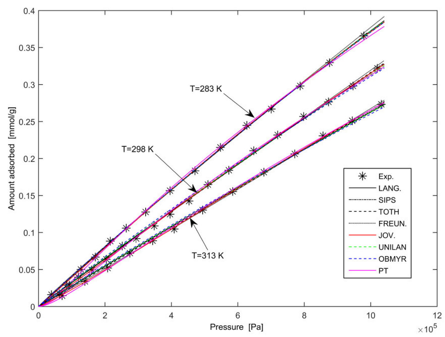
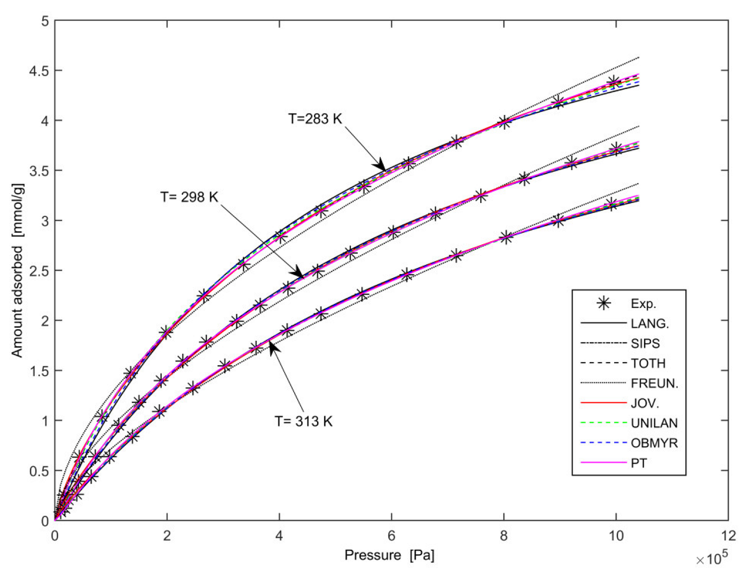
3.2. Pure-Gas Experimental Results

To carry out numerical experiments for pure gases, the experimental data of Wu et al. [27] have been chosen. The authors provided experimental data for adsorption of hydrogen (Figure 1), nitrogen (Figure 2) and methane (Figure 3) on the activated carbon JX101 at 283K, 298K and 313K. The models of Langmuir (LANG.), Freundlich (FREUN.), Sips (SIPS), Toth (TOTH), Jovanovic (JOV.), UNILAN (UNILAN), OBMR (OBMYR) as well as the Potential Theory (discussed in the previous section) are used to describe the pure-gas adsorption equilibrium. The pressure range is from 0 to 1 MPa for the measurements of pure-component adsorption.

The models for the single-component adsorption have been fitted to the experimental isotherms of pure CH₄, N₂ and H₂ by nonlinear regression. The estimated parameters for each component are listed (see

Table A1. Coefficients of the model equations obtained by nonlinear regression of experimental data for the hydrogen gas at different temperatures.

Equation	Parameters			R-Square
	${\mathit{Q}}_{\mathit{m}\mathit{a}\mathit{x}}$	$\mathit{b}\mathbf{\times }{\mathbf{10}}^{\mathbf{8}}$	$\mathit{n}$
At temperature $\mathit{T}=\mathbf{283} \mathit{K}$
Langmuir	4.130	9.917	N/A	0.9997
Sips	3.900	2.110	0.200	0.9997
Toth	3.956	10.480	0.9685	0.9996
Freundlich (K and n)	7.104 × 10−7		1.048	0.9994
Jovanovic	3.993	9.494	0.984	0.9996
UNILAN	4.006	6.435	1.140	0.9997
OBMR	4.020	1.709	3.095	0.9995
Potential Theory	4.139	6.229 × 1011	1.630	0.9997
At temperature $\mathit{T}=\mathbf{298} \mathit{K}$
Langmuir	3.687	9.243	N/A	0.9985
Sips	3.731	46.370	5.086	0.9991
Toth	3.547	9.081	1.504	0.9989
Freundlich	3.283 × 10−7		1.002	0.9983
Jovanovic	3.508	10.600	1.047	0.9993
UNILAN	3.969	2.808	1.463	0.9997
OBMR	3.606	3.414	1.889	0.9996
Potential Theory	3.811	6.708 × 1011	1.69	0.9993
At temperature $\mathit{T}=\mathbf{313} \mathit{K}$
Langmuir	3.026	9.42	N/A	0.9966
Sips	3.1	14.35	1.563	0.9967
Toth	2.892	9.536	1.169	0.9979
Freundlich	1.832 × 10−7		0.97331	0.9991
Jovanovic	3.088	10.27	1.056	0.9998
UNILAN	3.081	1.878	1.737	0.998
OBMR	3.248	3.229	1.812	0.9995
Potential Theory	3.418	7.211 × 1011	1.741	0.9996

,

Table A2. Coefficients of the model equations obtained by nonlinear regression of experimental data for the nitrogen gas at different temperatures.

Equation	Parameters			R-Square
	${\mathit{Q}}_{\mathit{m}\mathit{a}\mathit{x}}$	$\mathit{b}\mathbf{\times }{\mathbf{10}}^{\mathbf{7}}$	$\mathit{n}$
At temperature $\mathit{T}=\mathbf{283} \mathit{K}$
Langmuir	5.116	7.402	N/A	0.9991
Sips (LF)	5.039	7.687	1.016	0.9993
Toth	5.338	7.774	0.8918	0.9999
Freundlich (K and n)	1.145 × 10−4		1.4	0.9974
Jovanovic	4.921	5.224	0.8336	0.9998
UNILAN	5.134	6.282	1.03	0.9999
OBMR	5.449	6.248	1.03	0.9997
Potential Theory	5.501	6.926 × 109	1.769	0.9999
At temperature $\mathit{T}=\mathbf{298} \mathit{K}$
Langmuir	4.638	6.099	N/A	0.9999
Sips	4.638	6.214	1.019	0.9999
Toth	4.512	6.239	1.02	0.9995
Freundlich	3.581 × 10−5		1.275	0.9996
Jovanovic	4.5	4.654	0.8937	0.9994
UNILAN	5.25	4.334	1.03	0.9999
OBMR	4.964	1.58	2.244	0.9999
Potential Theory	4.876	7.208 × 109	1.823	0.9998
At temperature $\mathit{T}=\mathbf{313} \mathit{K}$
Langmuir	4.306	5.221	N/A	0.9996
Sips	4.308	6.554	1.256	0.9997
Toth	4.115	5.454	1.025	0.9997
Freundlich	2.714 × 10−5		1.265	0.9989
Jovanovic	4.324	3.791	0.8892	0.9998
UNILAN	4.525	3.589	1.079	0.9998
OBMR	4.159	5.477	0.004049	0.9997
Potential Theory	4.52	7.413 × 109	1.781	0.9998

and

Table A3. Coefficients of the model equations obtained by nonlinear regression of experimental data for the methane gas at different temperatures.

Equation	Parameters			R-Square
	${\mathit{Q}}_{\mathit{m}\mathit{a}\mathit{x}}$	$\mathit{b}\mathbf{\times }{\mathbf{10}}^{\mathbf{6}}$	$\mathit{n}$
At temperature $\mathit{T}=\mathbf{283} \mathit{K}$
Langmuir	6.367	2.073	N/A	0.9978
Sips	6.368	2.115	1.021	0.9979
Toth	6.4	2.149	0.9673	0.998
Freundlich (K and n)	2.147 × 10-3		1.805	0.9936
Jovanovic	6.214	1.293	0.7586	0.9997
UNILAN	6.206	1.68	1.062	0.9988
OBMR	6.5	1.98	0.3916	0.9982
Potential Theory	6.489	8.382 × 109	2.081	0.9992
At temperature $\mathit{T}=\mathbf{298} \mathit{K}$
Langmuir	3.041	1.541	N/A	0.9993
Sips	6.042	1.57	1.019	0.9993
Toth	7.025	1.463	0.8436	0.9997
Freundlich	7.772 × 10-4		1.624	0.9934
Jovanovic	6.021	0.984	0.776	0.9988
UNILAN	6.01	1.21	1.086	0.9997
OBMR	6.4	1.363	0.4485	0.9995
Potential Theory	6.2	8.288 × 109	2.013	0.9998
At temperature $\mathit{T}=\mathbf{313} \mathit{K}$
Langmuir	5.724	1.215	N/A	0.9996
Sips	5.724	1.368	1.126	0.9995
Toth	5.9	1.207	0.9611	0.9997
Freundlich	3.51 × 10-4		1.511	0.9996
Jovanovic	4.553	1.207	0.8881	0.9998
UNILAN	5.901	0.921	1.054	0.9998
OBMR	5.805	0.243	2.66	0.9983
Potential Theory	5.93	8.302 × 109	1.94	1.0000

in Appendix A). The goodness of fit is expressed by the square of the multiple correlation coefficient (R-Square) between the response values and the predicted response values.

$$R-Square=1-\frac{{\displaystyle \sum _{i=1}^n{\left(x_i-{\widehat{x}}_i\right)}^2}}{{\displaystyle \sum _{i=1}^n{\left(x_i-{\overline{x}}_i\right)}^2}}$$

(7)

where $\widehat{x}$ is the predicted response value and $\overline{x}$ is the average value. R-square can take on any value between 0 and 1, with a value closer to 1 indicating that a greater proportion of variance is accounted for by the model.

A comparison of the experimental data with the correlation results for pure-hydrogen adsorption isotherms is illustrated in Figure 1.

In this pressure range, a linear behaviour is observed for the hydrogen adsorption equilibrium data. The parameters and the R-Square deviation are given in Table A1 in the Appendix A. The R-Square of these models is greater than $0.99$ for the tested range, which means that these isotherm models fit quite well to the adsorption equilibrium data of single components.

A comparison between the modelled results and the experimental data for the pure-nitrogen gas adsorption equilibrium is presented in Figure 2. In Table A2 in the Appendix A, the parameters and R-Square deviation obtained by nonlinear regression of experimental data are given. As can be observed from Figure 2, some deviations appear between experimental data and correlation results from the Freundlich model, especially for high pressures and low temperatures, but these deviations are very small and we can conclude that all the models describe the experimental results with satisfactory accuracy.

A comparison between experimental and estimated results for the methane gas adsorption equilibrium is shown in Figure 3. The fit parameters are given in Table A3 in the Appendix A. In this pressure range, the isotherms follow the first type according to the IUPAC classification [46]. In the same way as for the nitrogen gas adsorption, small differences between Freundlich’s modelling results and experimental data are observed. The R-Square deviations for all modelling results are above 0.99. Thus, the eight models give satisfactory results for the methane gas adsorption equilibrium.

The curve for methane offers a greater curvature than the one for nitrogen, which indicates a stronger interaction between methane and activated carbon than between nitrogen and activated carbon. The same result has been observed when comparing nitrogen and hydrogen adsorption equilibria. This fact was also confirmed in the results of numerical experiments. The affinity constant $b$ corresponds to the force of the interaction between adsorbed molecules and the adsorbent solid surface. A greater value of $b$ corresponds to a stronger area interaction. For example, in Toth’s model, average values of $b$ at 298 K for hydrogen, nitrogen and methane are $9.081\times {10}^{-8}$, $6.239\times {10}^{-7}$ and $1.463\times {10}^{-6}$, respectively (Table A1, Table A2 and Table A3 in Appendix A). Thus, the interactions between methane gas and activated carbon are the strongest, followed by nitrogen and hydrogen.

To conclude, in the case of pure-gas adsorption, the adsorbate–adsorbent interactions are more significant than the adsorbate–adsorbate interactions.

4. Conclusions

The adsorption equilibria of hydrogen, nitrogen and methane gases on activated carbon JX101 at three different temperatures (283 K, 298 K and 313 K) have been described. The calculations were carried out in the programming environment MATLAB R2011a which develops the relevant file functions and software communication links for the mathematical models used.

To calculate the necessary physico-chemical parameters (pseudo-saturation vapour pressure and molar volume of the adsorbate), several thermodynamic models have been tested. In order to estimate the fugacity, the Soave–Benedict–Webb–Rubin Equation of State has been selected. Two models for the pseudo-vapour pressure determination have also been tested. The model of Dubinin has been selected as more suitable. A brief review of the advantages and disadvantages of different models for calculating the molar volume of the adsorbed phase has been conducted. Based on the results obtained to estimate the adsorbed phase molar volume, the model proposed by Do has been selected.

Eight models to describe the adsorption equilibria of pure gases on microporous adsorbents have been tested by comparison with experimental data proposed by Wu et al. [27]. Except for Freundlich’s equation in the case of nitrogen or methane adsorption, all the models used in this paper provide a good agreement between experimental and calculated values of the adsorption isotherms.

References

1. Yue, B.; Liu, S.; Chai, Y.; Wu, G.; Guan, N.; Li, L. Zeolites for separation: Fundamental and application. J. Energy Chem. 2022, 71, 288–303. [Google Scholar] [CrossRef]
2. Sayılgan, Ş.Ç.; Mobedi, M.; Ülkü, S. Effect of regeneration temperature on adsorption equilibria and mass diffusivity of zeolite 13x-water pair. Micropor. Mesopor. Mat. 2016, 224, 9–16. [Google Scholar] [CrossRef] [Green Version]
3. Zeng, W.; Xu, L.; Wang, Q.; Chen, C.; Fu, M. Adsorption of Indium(III) Ions from an Acidic Solution by Using UiO-66. Metals 2022, 12, 579. [Google Scholar] [CrossRef]
4. Zhang, X.; Zheng, Q.R.; He, H.Z. Multicomponent adsorptive separation of CO2, CH4, N2, and H2 over M-MOF-74 and AX-21@ M-MOF-74 composite adsorbents. Micropor. Mesopor. Mat. 2022, 336, 111899. [Google Scholar] [CrossRef]
5. Chumakova, L.S.; Bakulin, A.V.; Hocker, S.; Schmauder, S.; Kulkova, S.E. Interaction of Oxygen with the Stable Ti5Si3 Surface. Metals 2022, 12, 492. [Google Scholar] [CrossRef]
6. Weinberger, B.; Darkrim Lamari, F.; Levesque, D. Capillary condensation and adsorption of binary mixtures. J. Chem. Phys. 2006, 124, 234712. [Google Scholar] [CrossRef] [Green Version]
7. Kumar, K.V.; Gadipelli, S.; Howard, C.A.; Kwapinski, W.; Brett, D.J. Probing adsorbent heterogeneity using Toth isotherms. J. Mater. Chem. A 2021, 9, 944–962. [Google Scholar] [CrossRef]
8. Goswami, A.; Ma, H.; Schneider, W.F. Consequences of adsorbate-adsorbate interactions for apparent kinetics of surface catalytic reactions. J. Catal. 2022, 405, 410–418. [Google Scholar] [CrossRef]
9. Cho, Y.; Lo, R.; Krishnan, K.; Yin, X.; Kazemi, H. Measuring Absolute Adsorption in Porous Rocks Using Oscillatory Motions of a Spring-Mass System. Chin. J. Chem. Eng. 2022, 4, 131–139. [Google Scholar] [CrossRef]
10. Chen, L.; Liu, K.; Jiang, S.; Huang, H.; Tan, J.; Zuo, L. Effect of adsorbed phase density on the correction of methane excess adsorption to absolute adsorption in shale. Chem. Eng. J. 2021, 420, 127678. [Google Scholar] [CrossRef]
11. Ekundayo, J.M.; Rezaee, R.; Fan, C. Experimental investigation and mathematical modelling of shale gas adsorption and desorption hysteresis. J. Nat. Gas Sci. Eng. 2021, 88, 103761. [Google Scholar] [CrossRef]
12. Keller, J.U.; Staudt, R. Gas Adsorption Equilibria: Experimental Methods and Adsorptive Isotherms; Springer Science and Business Media: Boston, MA, USA, 2005; pp. 359–413. [Google Scholar]
13. Do, D.D.; Do, H.D. Adsorption of supercritical fluids in non-porous and porous carbons: Analysis of adsorbed phase volume and density. Carbon 2003, 41, 1777–1791. [Google Scholar] [CrossRef]
14. Chilev, C.; Darkrim Lamari, F.; Kirilova, E.; Pentchev, I. Comparison of gas excess adsorption models and high pressure experimental validation. Chem. Eng. Res. Des. 2012, 90, 2002–2012. [Google Scholar] [CrossRef]
15. Langmuir, I. The adsorption of gases on plane surfaces of glass, mica and platinum. J. Amer. Chem. Soc. 1918, 40, 1361–1403. [Google Scholar] [CrossRef] [Green Version]
16. Zeldowitsch, J. Adsorption site energy distribution. Acta Phys. Chim. URSS 1934, 1, 961–973. [Google Scholar]
17. Freundlich, H.M.F. Over the adsorption in solution. J. Phys. Chem. 1906, 57, 385–471. [Google Scholar] [CrossRef] [Green Version]
18. Sips, R. The Structure of a Catalyst Surface. J. Chem. Phys. 1948, 16, 490–495. [Google Scholar] [CrossRef]
19. Tóth, J. Gas-(Steam-) Adsorption on solid surfaces of inhomogeneous activity III. Acta Chim. Acad. Sci. Hung. 1962, 32, 39–57. [Google Scholar]
20. Jovanovic, D.S. Physical adsorption of gases—II: Practical application of derived isotherms for monolayer and multilayer adsorption. Kollozd Z. 1969, 235, 1214–1225. [Google Scholar] [CrossRef]
21. Quinones, I.; Guiochon, G. Extension of a Jovanovic–Freundlich isotherm model to multicomponent adsorption on heterogeneous surfaces. Chromatogr. J. 1998, 796, 15–40. [Google Scholar] [CrossRef]
22. Hazlett, J.D.; Hsu, C.C.; Wojciechowski, B.W. Is the Jovanovic isotherm theoretically valid? J. Chem. Soc. Faraday Trans 2 1979, 75, 602–605. [Google Scholar] [CrossRef]
23. Grady, C.; McWhorter, S.; Sulic, M.; Sprik, S.J.; Thornton, M.J.; Brooks, K.P.; Tamburello, D.A. Design tool for estimating adsorbent hydrogen storage system characteristics for light-duty fuel cell vehicles. Int. J. Hydrog. Energ. 2022, 47, 29847–29857. [Google Scholar] [CrossRef]
24. O’Brien, J.A.; Myers, A.L. Physical adsorption of gases on heterogeneous surfaces. Series expansion of isotherms using central moments of the adsorption energy distribution. J. Chem. Soc. Faraday Trans. 1 1984, 80, 1467–1477. [Google Scholar] [CrossRef]
25. Bering, B.P.; Dubinin, M.M.; Serpinsky, V.V. On thermodynamics of adsorption in micropores. J. Colloid. Int. Sci. 1972, 38, 185–194. [Google Scholar] [CrossRef]
26. Dubinin, M.M.; Radushkevich, L.V. The equation of the characteristic curve of the activated charcoal. Proc. Acad. Sci. USSR Phys. Chem. Sect. 1947, 55, 331–337. [Google Scholar]
27. Wu, Q.; Zhou, L.; Wu, J.; Zhou, Y. Adsorption equilibrium of the mixture CH4+N2+H2 on activated carbon. J. Chem. Eng. Data 2005, 50, 635–642. [Google Scholar] [CrossRef]
28. Chilev, C.; Darkrim Lamari, F. Hydrogen storage at low temperature and high pressure for application in automobile manufacturing. Int. J. Hydrog. Energ. 2016, 41, 1744–1758. [Google Scholar] [CrossRef]
29. van der Waals, J.D. Over de Continuited van den Gas-en Vloeistoftoestand. Ph.D. Thesis, University of Leiden, Holland, The Netherlands, 14 June 1873. [Google Scholar]
30. Peng, D.Y.; Robinson, D.B. A New Two-Constant Equation of State. Ind. Eng. Chem. Fundam. 1976, 15, 59–64. [Google Scholar] [CrossRef]
31. Patel, N.C.; Teja, A.S. A new cubic equation of state for fluids and fluid mixtures. Chem. Eng. Sci. 1982, 37, 463–473. [Google Scholar] [CrossRef]
32. McCarty, R.D.; Weber, L.A. Thermophysical properties of parahydrogen from the freezing liquid line to 5000 R for pressures to 10,000 psia. In National Bureau of Standards—Technical Note 617; NBS: Boulder, CO, USA, 1972; pp. 1–169. [Google Scholar]
33. Lemmon, E.W.; McLinden, M.O.; Friend, D.G. Thermophysical properties of fluid systems. In the NIST Chemistry Webbook; Database Reference Number 69; National Institute of Standards and Technology: Gaithersburg, MD, USA, 1998. [Google Scholar] [CrossRef]
34. Dubinin, M.M. Modern state of the theory of gas and vapour adsorption by microporous adsorbents. Pure Appl. Chem. 1965, 10, 309–322. [Google Scholar] [CrossRef]
35. Dubinin, M.M.; Fomkin, A.F.; Seliverstova, I.I.; Serpinsky, V.V. Direct determination of the density of adsorbates in zeolite micropores. In Proceedings of the Fifth Int. Conference on Zeolite, Naples, Italy, 2–6 June 1980. [Google Scholar]
36. Rogers, K.A. Adsorption on Activated Carbon of Hydrogen, Methane, and Carbon Dioxide gases and Their Mixtures at 212–301 Degrees K and up to Thirty-Fie Atmospheres. Ph.D. Thesis, Georgia Institute of Technology, Atlanta, GA, USA, 1973. [Google Scholar]
37. Findenegg, G. High-pressure physical adsorption of gases on homogeneous surfaces. In Fundamentals of Adsorption; Myers, A.L., Belfort, G., Eds.; United Engineering Trustees: New York, NY, USA, 1984; Volume 1, pp. 207–218. [Google Scholar]
38. Mehta, S.D.; Danner, R.P. An improved potential theory method for predicting gas-mixture adsorption equilibria. Ind. Eng. Chem. Fund. 1985, 24, 325–330. [Google Scholar] [CrossRef]
39. Dubinin, M.M. The potential theory of adsorption of gases and vapors for adsorbents with energetically non-uniform surfaces. Chem. Rev. 1960, 60, 235–241. [Google Scholar] [CrossRef]
40. Ozawa, S.; Kusumi, S.; Ogino, Y. Physical adsorption of gases at high pressure. IV. An improvement of the Dubinin—Astakhov adsorption equation. J. Coll. Int. Sci. 1976, 56, 83–91. [Google Scholar] [CrossRef]
41. Dubinin, M.M. Physical adsorption of gases and vapors in micropores. In Progress in Surface and Membrane Science, 1st ed.; Cadenhead, D.A., Danielli, J.E., Rosenberg, M.D., Eds.; Academic Press: New York, NY, USA, 1975; Volume 9, pp. 1–70. [Google Scholar]
42. Do, D.D. Adsorption Analysis: Equilibria and kinetics; Imperial College Press: London, UK, 1998. [Google Scholar]
43. Maslan, F.D.; Altman, M.; Alberth, E.R. Prediction of Gas–Adsorbent Equilibria. J. Phys. Chem. 1953, 57, 106–109. [Google Scholar] [CrossRef]
44. Lewis, W.K.; Gilliland, E.R.; Chertow, L.; Cadogen, W.P. Adsorption equilibria hydrocarbon gas mixtures. Ind. Eng. Chem. 1950, 42, 1319–1326. [Google Scholar] [CrossRef]
45. Grant, R.J.; Manes, M. Adsorption of normal paraffins and sulfur compounds on activated carbon. AIChE J. 1962, 8, 403–406. [Google Scholar] [CrossRef]
46. Cook, W.H.; Basmadjian, D. Correlation of adsorption equilibria of pure gases on activated carbon. Can. J. Chem. Eng. 1964, 42, 146–151. [Google Scholar] [CrossRef]
47. Sing, K.S.W. Reporting physisorption data for gas/solid systems with special reference to the determination of surface area and porosity (Recommendations 1984). Pure Appl. Chem. 1985, 57, 603–618. [Google Scholar] [CrossRef]
Figure 1. Pure-hydrogen adsorption results on activated carbon JX101.
Metals 12 01698 g001
Figure 2. Pure-nitrogen adsorption results on activated carbon JX101.
Metals 12 01698 g002
Figure 3. Pure-methane adsorption results on activated carbon JX101.
Metals 12 01698 g003