
A New Prediction Method for the Preload Drag Force of Linear Motion Rolling Bearing

Abstract
:1. Introduction
2. Experiment
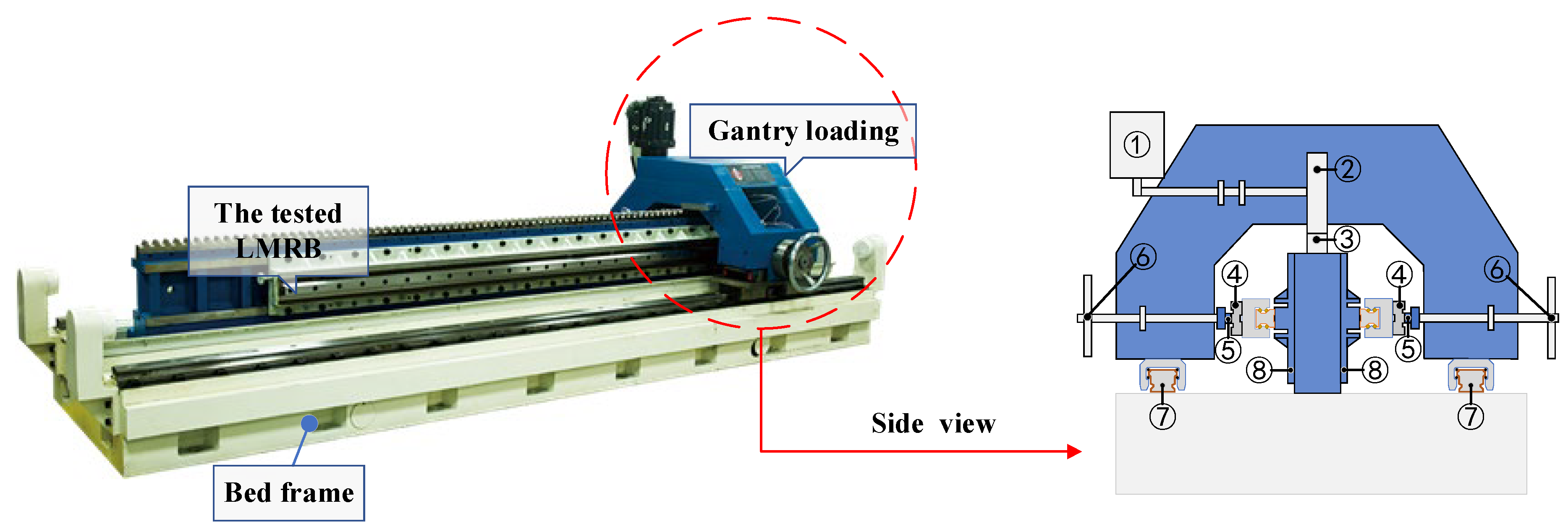
2.1. Loading Test
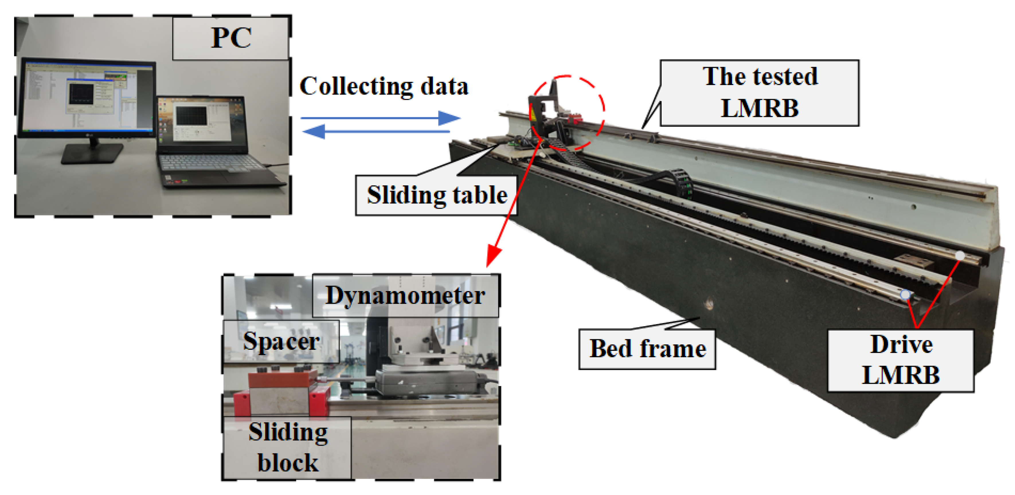
2.2. Preload Drag Force Measurement
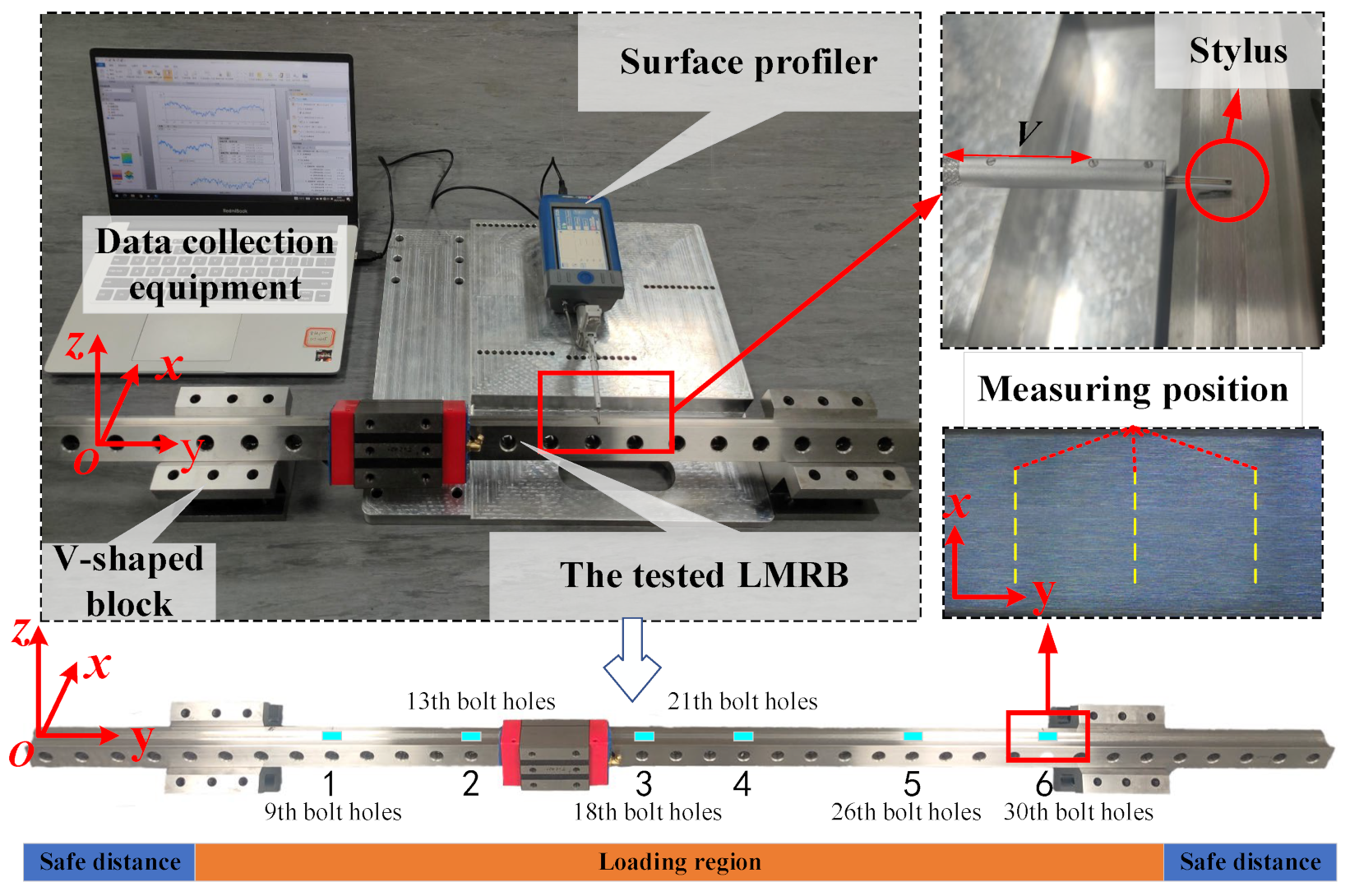
2.3. Raceway Topography Measurement
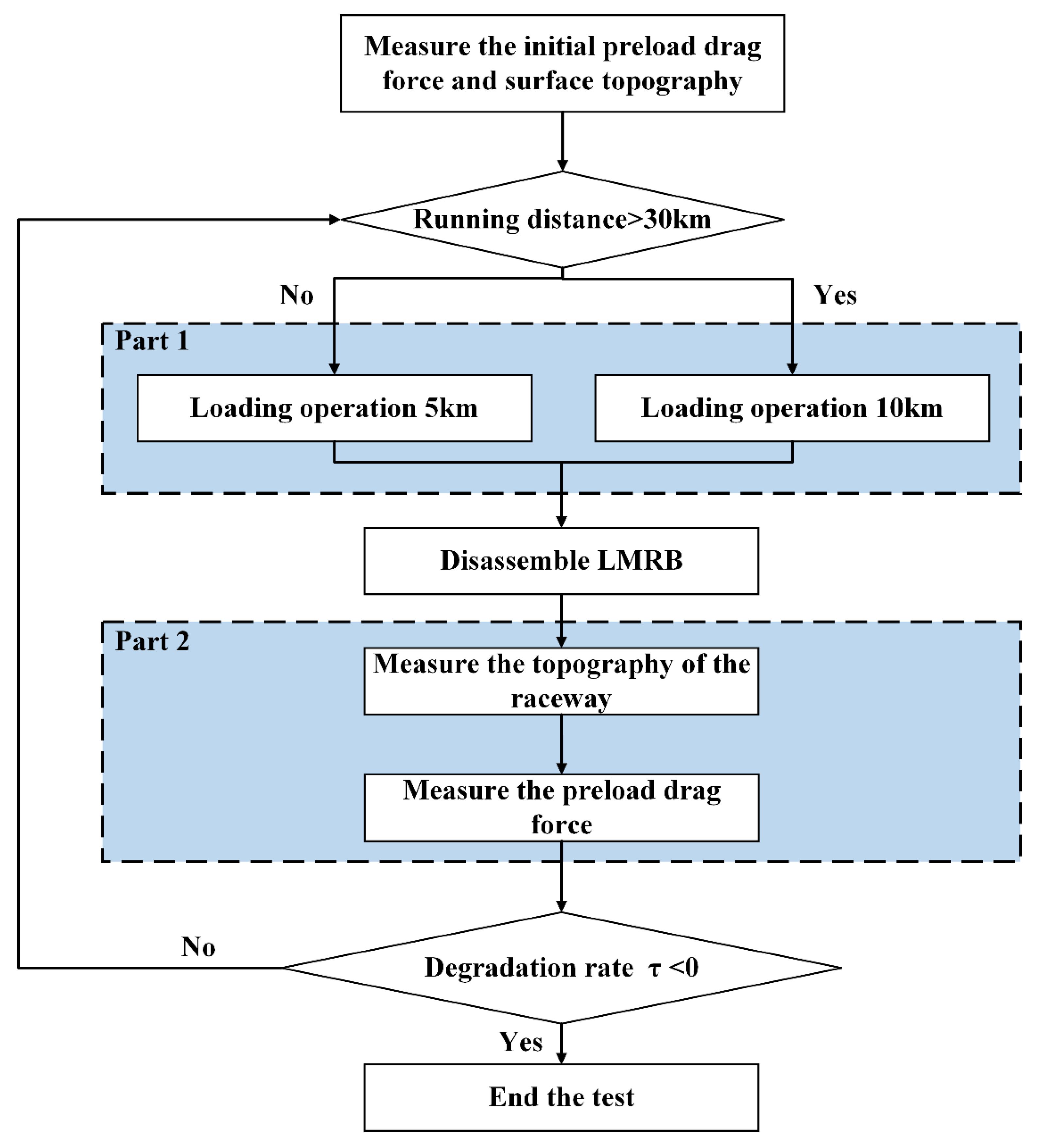
2.4. Test Procedure
3. Results
3.1. Preload Drag Force Degradation
3.2. Change in Raceway Topography
3.3. Two-Dimensional Profile of a Raceway Surface
3.3.1. Statistical Parameters
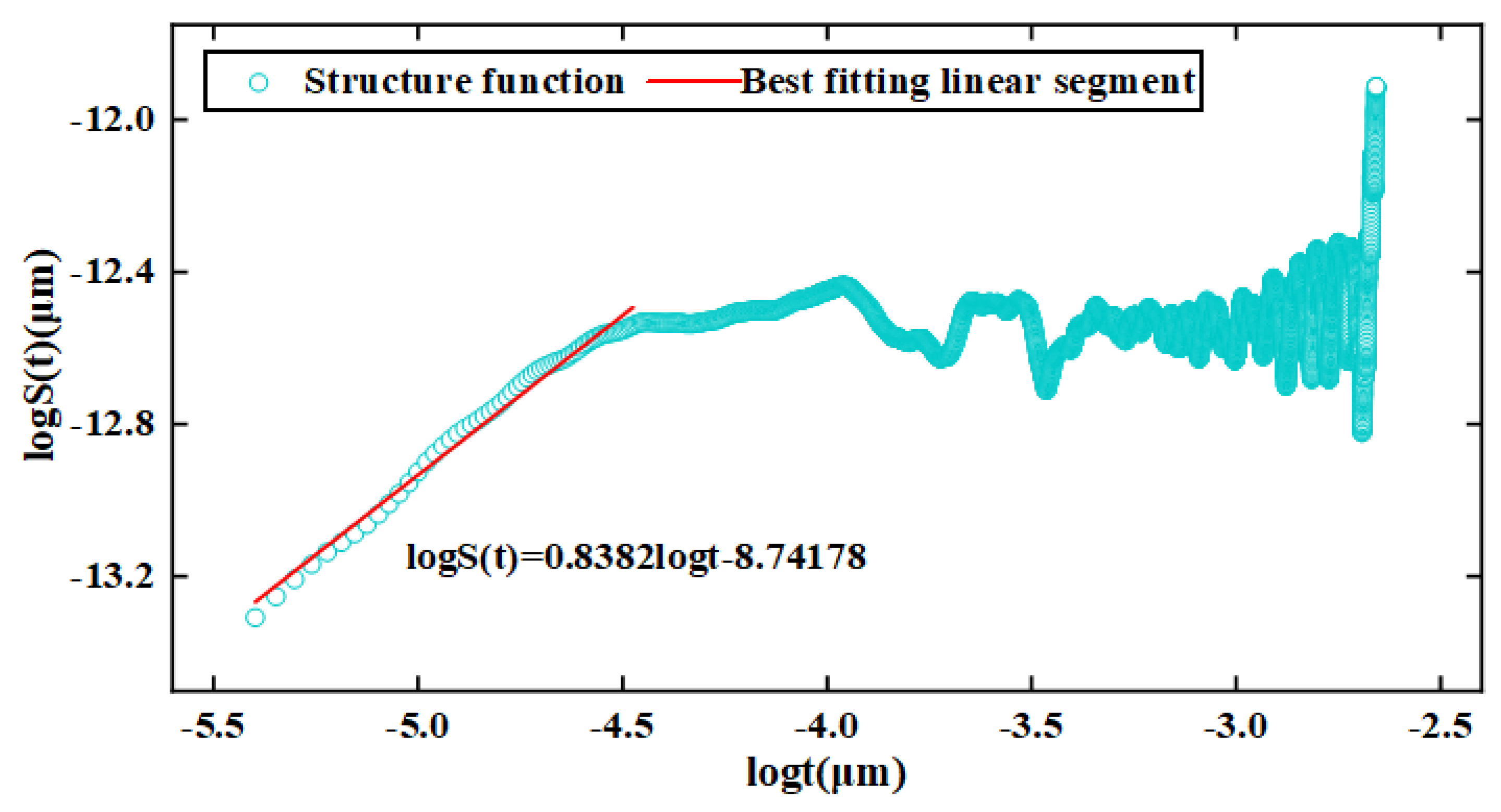
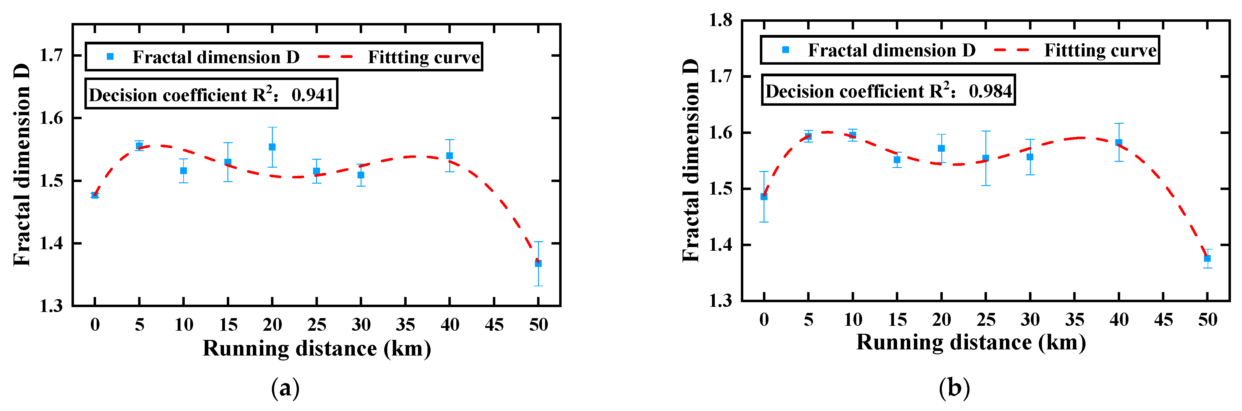
3.3.2. Fractal Parameters
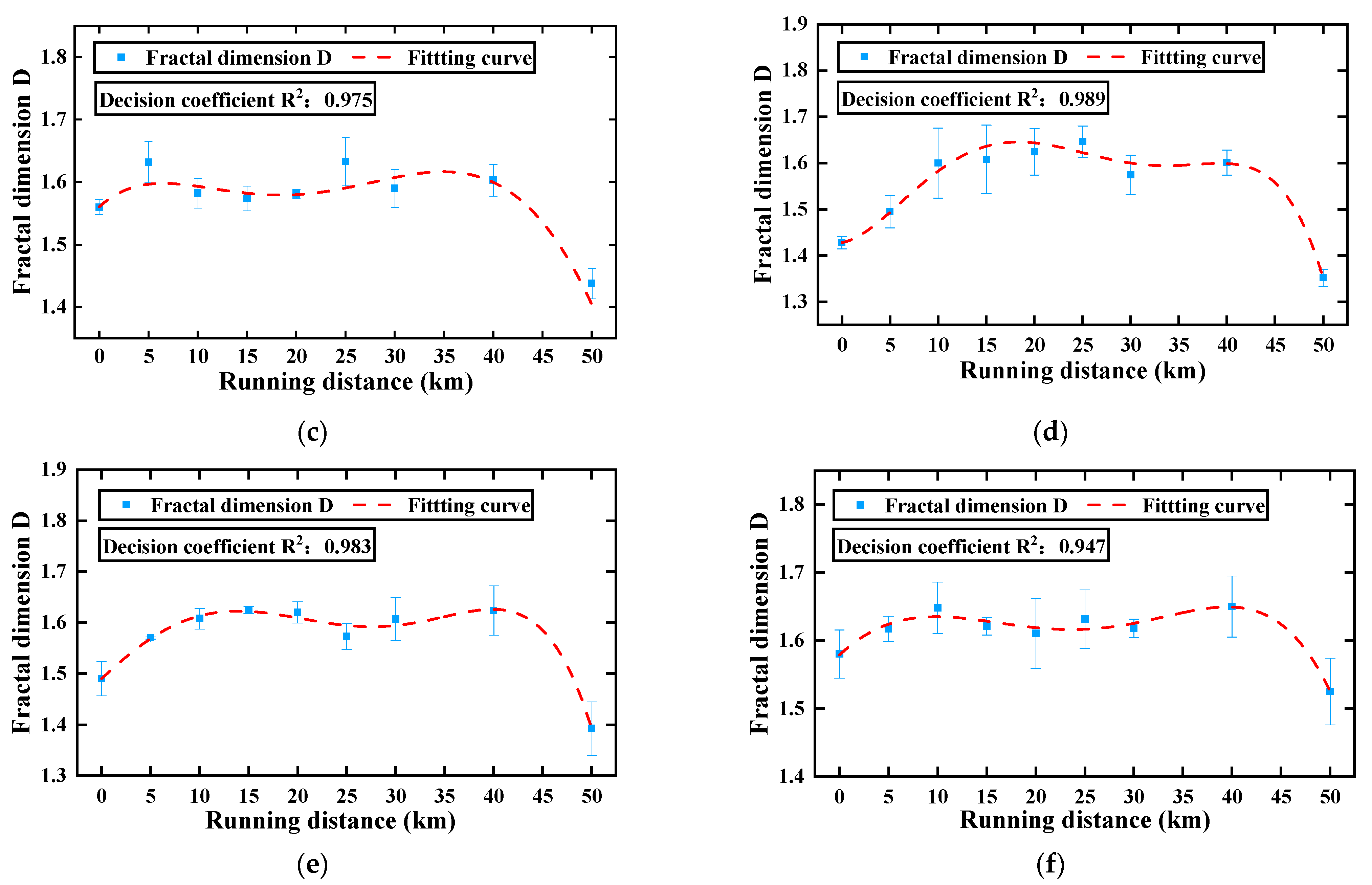
3.3.3. Recursive Analysis
4. Correlation Study
4.1. Establishing Correlation
4.2. Gray Correlation
5. Preload Prediction
5.1. Gaussian Regression Process Model of Preload Drag Force
5.2. Gaussian Regression Model Training and Prediction Analysis
5.2.1. Gaussian Regression Model Training
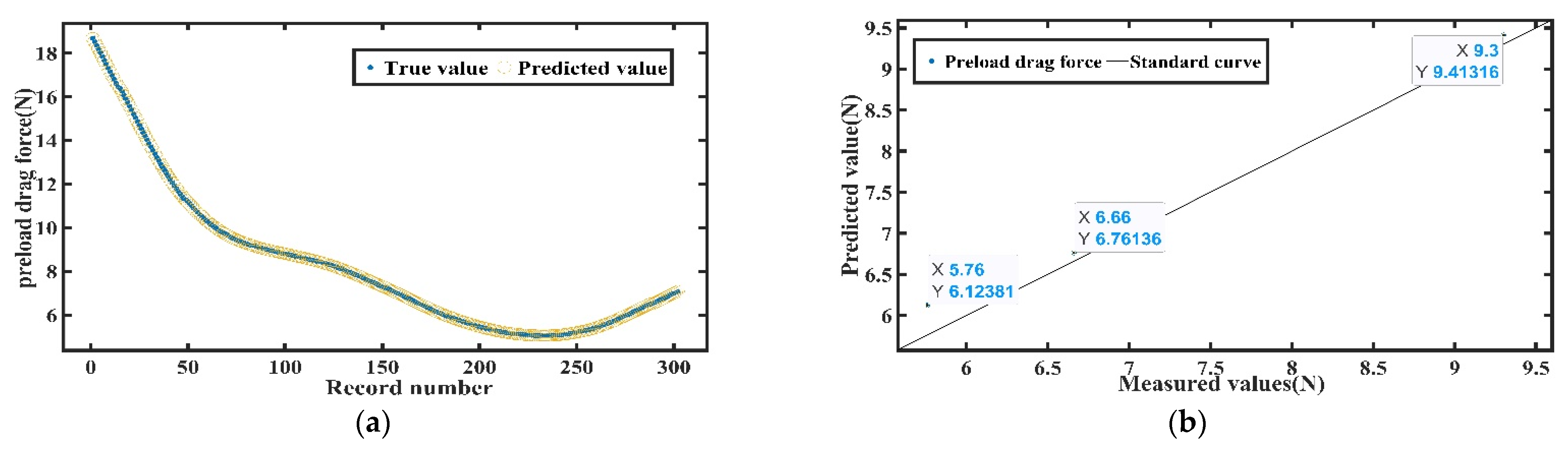
5.2.2. Prediction and Test Comparison of Preload Drag Force
6. Conclusions
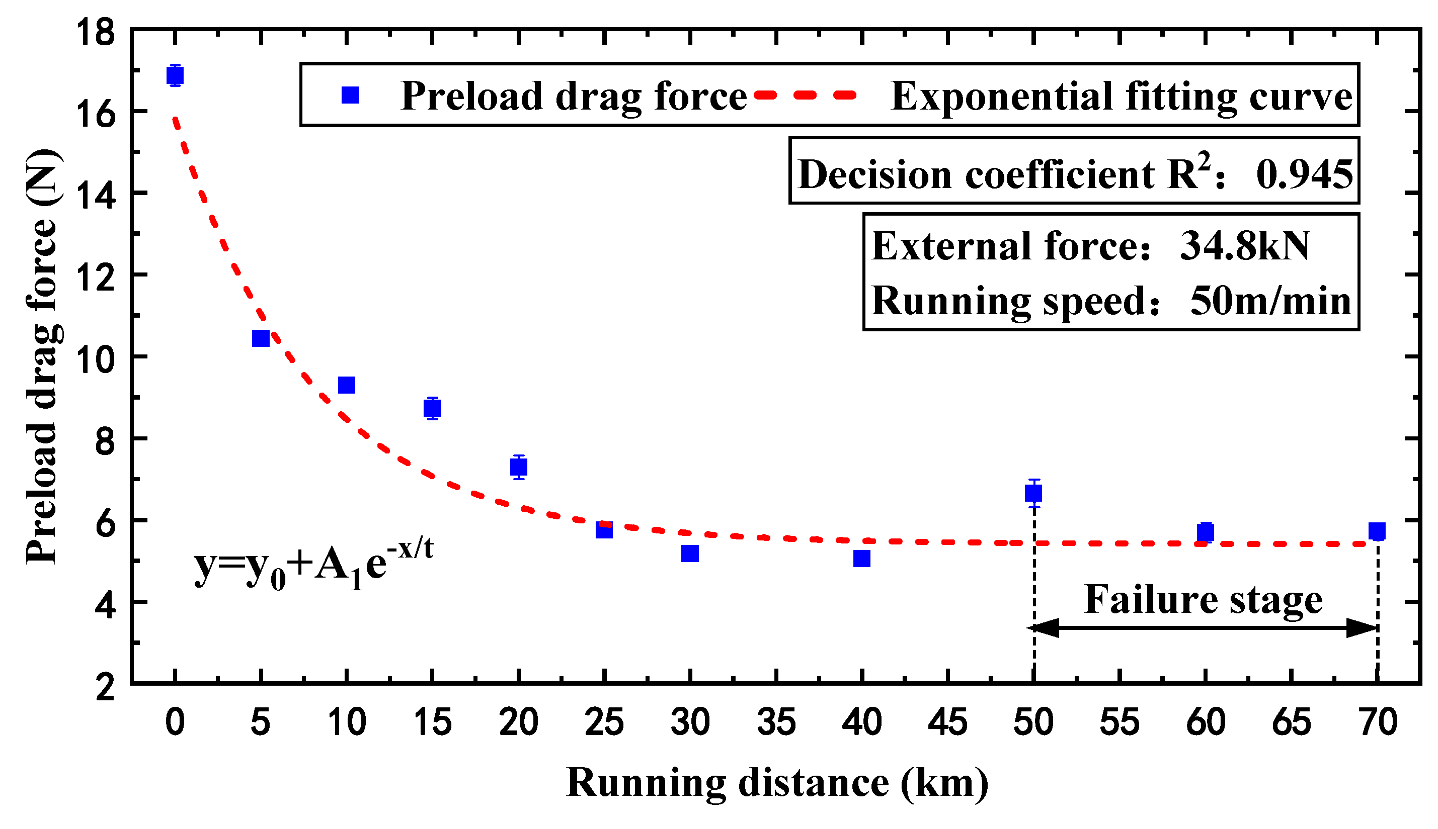
- The degradation in preload drag force of the LMRB is divided into three stages: rapid descent, slow descent, and failure.
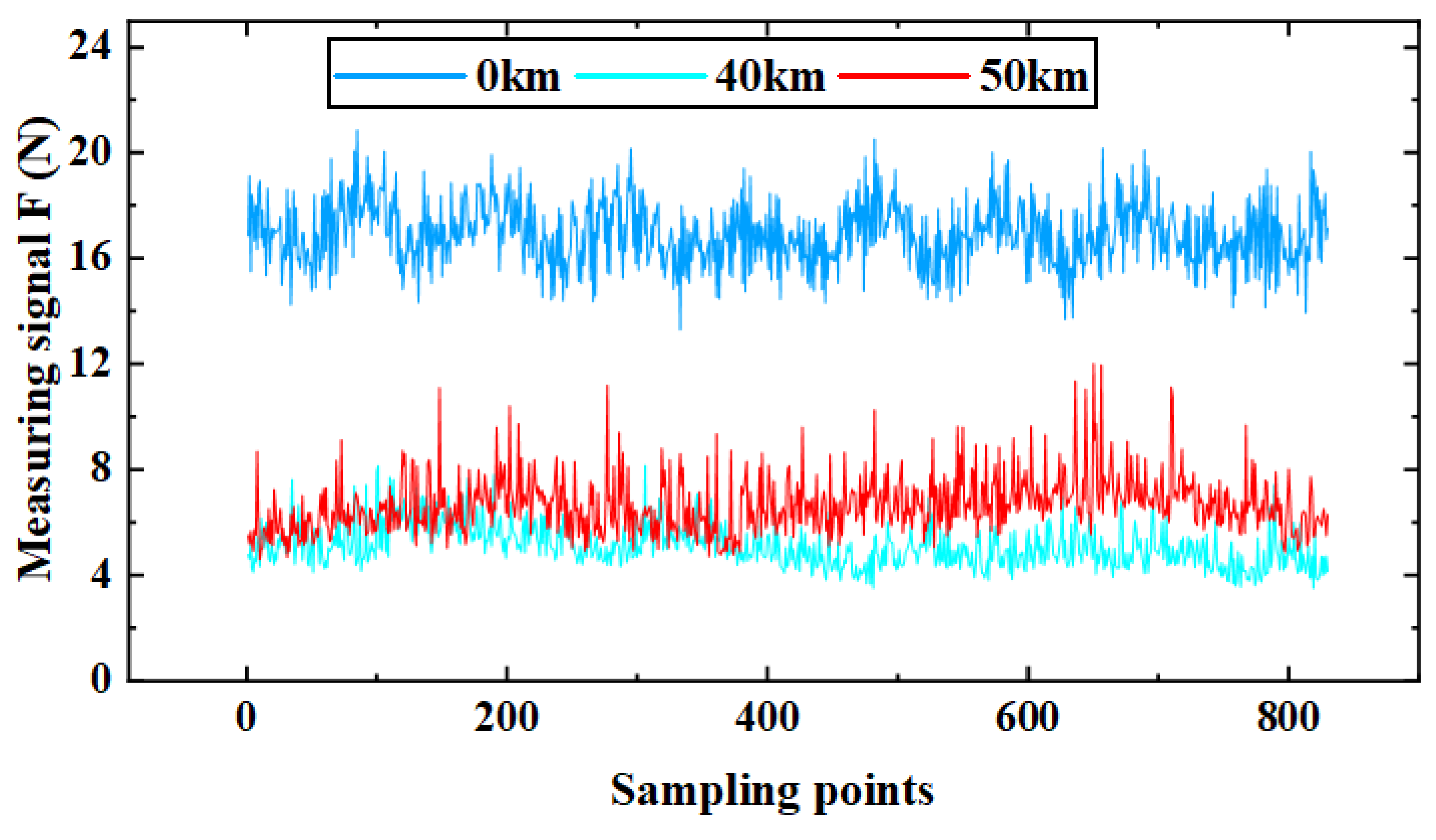
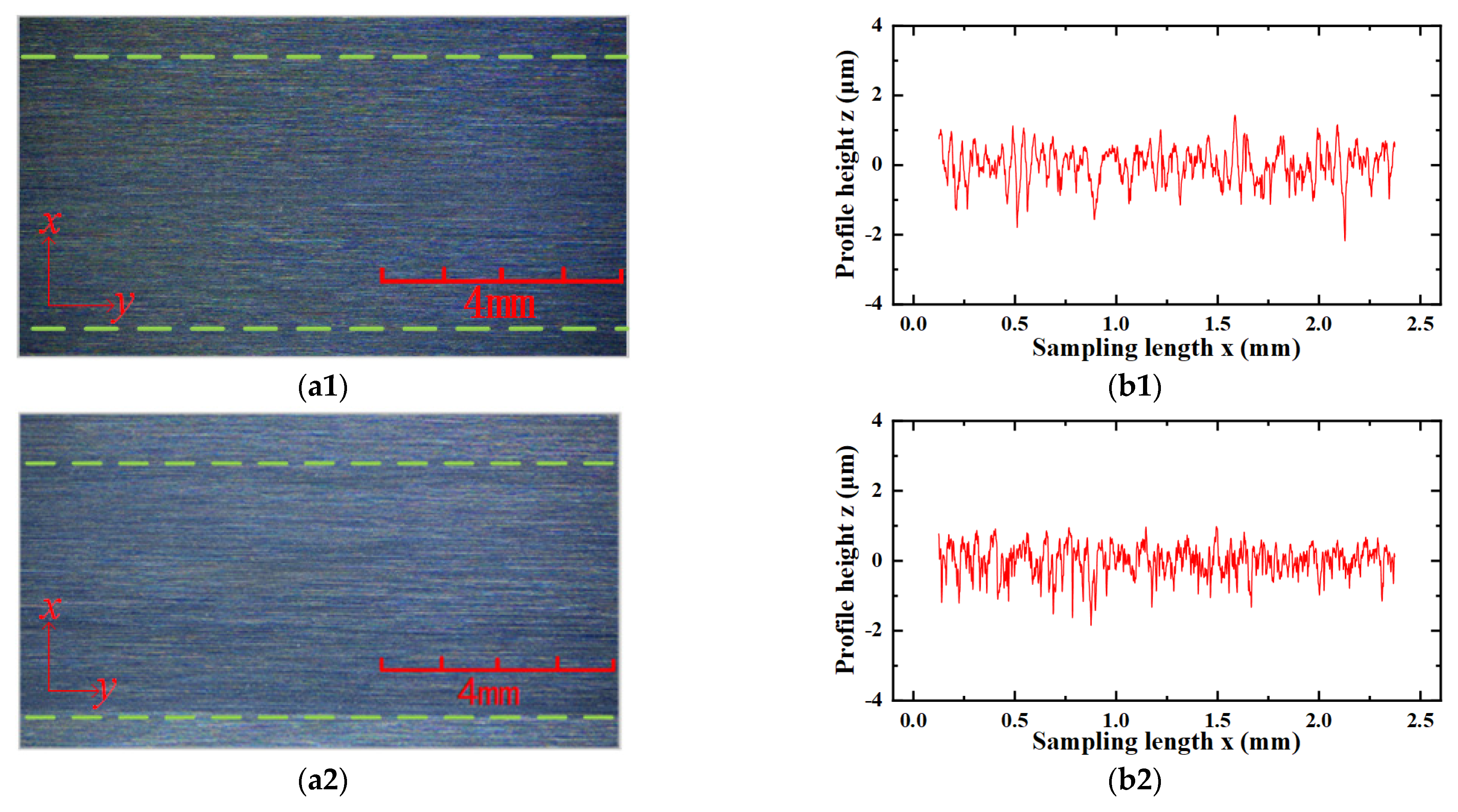
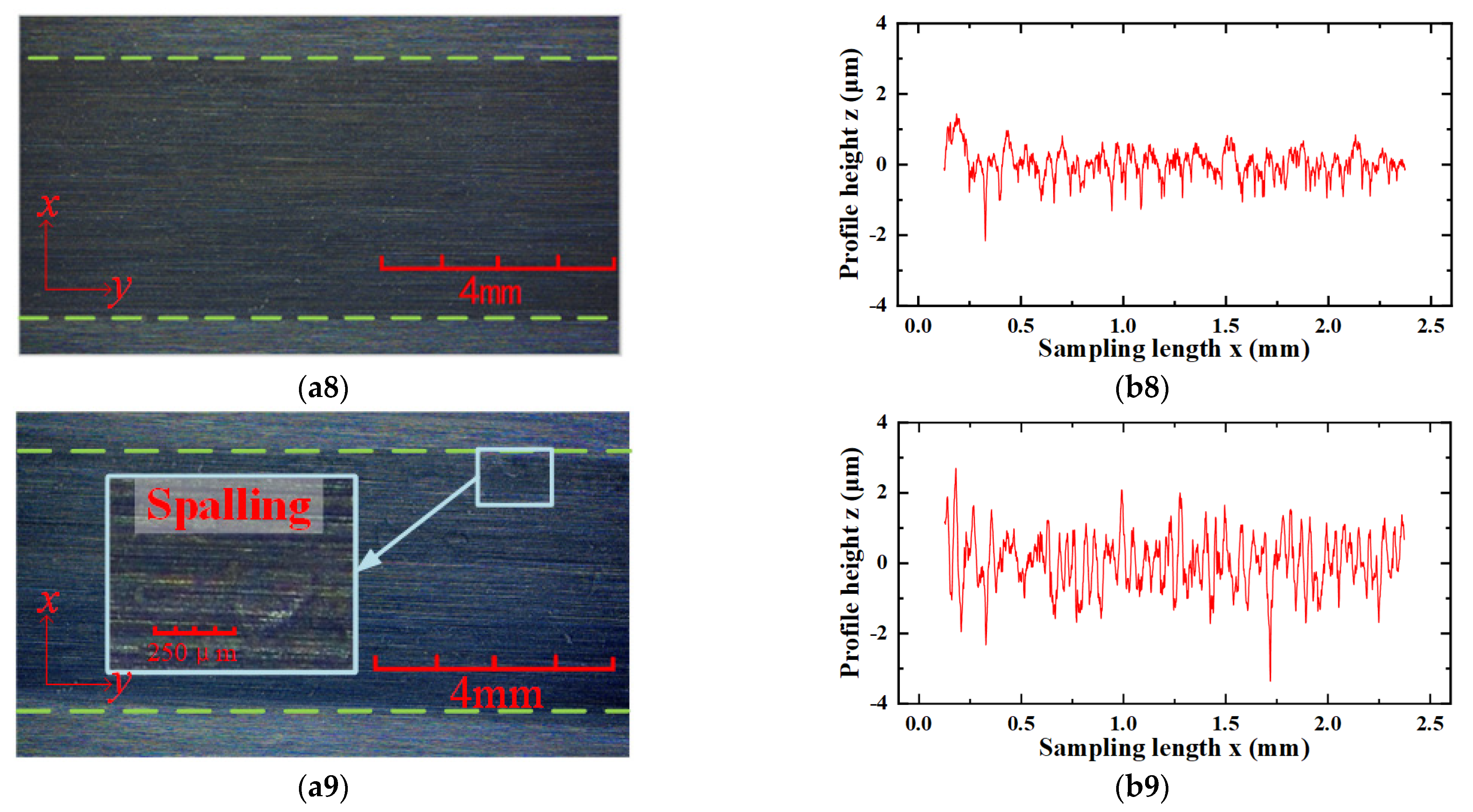
- Comparing the variation in preload drag force with the microscopic images and two-dimensional profile of the raceway surface shows that the raceway morphology reflects the degradation state of its preload drag force.
- The four parameters Ra, Rt, D, and Rr effectively represent the variational law of raceway morphology. The variational trends of Ra and Rt are “bathtub shaped”, and the variational trends of the fractal dimension D and recurrence rate Rf show an “inverted bathtub shape”. This conclusion provides a new way to monitor the degradation of the preload drag force of an LMRB.
- Gray correlation analysis of the degradation trend of the preload drag force yields correlations of 0.645, 0.657, 0.718, and 0.722 for the four characteristic parameters Ra, Rt, D, and Rr, respectively. Rr was recognized as optimal characterizing parameter.
- By using the Gaussian process regression theory, a regression model of the preload drag force is constructed on the basis of the rolling track topography of LMRB. The accuracies of prediction results of the three sets are 93.75%, 98.5%, and 98.8%, respectively, which validates the accuracy of the proposed model. This model describe in this paper can be utilized efficiently for the prediction of LMRB preload drag force degradation based on rolling morphology.
Author Contributions
Funding
Data Availability Statement
Conflicts of Interest
References
- Tong, V.; Khim, G.; Hong, S.; Park, C.H. Construction and validation of a theoretical model of the stiffness matrix of a linear ball guide with consideration of carriage flexibility. Mech. Mach. Theory 2019, 140, 123–143. [Google Scholar] [CrossRef]
- Chen, C.; Li, B.; Guo, J.; Liu, Z.; Qi, B.; Hua, C. Bearing life prediction method based on the improved FIDES reliability model. Reliab. Eng. Syst. Saf. 2022, 227, 108746. [Google Scholar] [CrossRef]
- Sun, W.; Kong, X.; Wang, B.; Li, X. Statics modeling and analysis of LMRB way considering rolling balls contact. Proceedings of the Institution of Mechanical Engineers. Part C J. Mech. Eng. Sci. 2015, 229, 168–179. [Google Scholar] [CrossRef]
- Li, D.; Liu, X.; Li, L.; Guo, G. Influence of Geometric Parameters on Lubrication Performance of Rolling Linear Guides Considering Stiffness Effects. J. Mech. Eng. 2021, 57, 100–108. [Google Scholar] [CrossRef]
- Han, J.; Dai, L. Research on Interchangeability Technology of Low Preload Rolling Linear Guide Pair. Sci. Technol. Vis. 2018, 25, 23–24+53. [Google Scholar] [CrossRef]
- Qi, B.; Zhao, J.; Chen, C.; Song, X.; Jiang, H. Accuracy decay mechanism of ball screw in CNC machine tools for mixed sliding-rolling motion under non-constant operating conditions. Int. J. Adv. Manuf. Technol. 2022. [Google Scholar] [CrossRef]
- Gu, Q.; Liang, Y.; Ren, X.; Feng, H.; Zhou, C. Relation between Friction Force and Static Stiffness of Roller Guide. Modul. Mach. Tool Autom. Manuf. Tech. 2020, 67–71+75. [Google Scholar] [CrossRef]
- Ren, S.; Zhou, C.; Ye, K.; Feng, H.-T.; Zhang, Y.-S. Calculating and Experiment Study on Friction Coefficient of LMRB. Tribology 2022, 42, 305–313. [Google Scholar] [CrossRef]
- Cheng, D.J.; Yang, W.S.; Park, J.H.; Park, T.J.; Kim, S.J.; Kim, G.H.; Park, C.H. Friction experiment of linear motion roller guide THK SRG25. Int. J. Precis. Eng. Manuf. 2014, 15, 545–551. [Google Scholar] [CrossRef]
- Oh, K.; Khim, G.; Park, C.; Chung, S.C. Explicit modeling and investigation of friction forces in linear motion ball guides. Tribol. Int. 2019, 129, 16–28. [Google Scholar] [CrossRef]
- Zhou, C.; Ren, S.; Feng, H.; Shen, J.-W.; Zhang, Y.-S.; Chen, Z.T. A new model for the preload degradation of LMRB. Wear 2021, 482–483, 203963. [Google Scholar] [CrossRef]
- Huang, H.; Gao, H.; Xu, M.; Zhang, X.; Guo, L. Performance Degradation Evaluation Method of CNC Machine Tool Spindle System. J. Vib. Meas. Diagn. 2013, 33, 646–652+726. [Google Scholar] [CrossRef]
- Yang, X.; Wu, J.; Ma, J. Rolling bearing performance degradation assessment method based on dispersion entropy and cosine Euclidean distance. J. Electron. Meas. Instrum. 2020, 34, 15–24. [Google Scholar] [CrossRef]
- Cheng, R.; Ou, Q.; Feng, H. Study on the Influence of Preload to Vibration of Roller Linear Guide Pairs. Modul. Mach. Tool Autom. Manuf. Tech. 2018, 03, 11–13+18. [Google Scholar] [CrossRef]
- Liu, X. Correlation analysis of surface topography and its mechanical properties at micro and nanometre scales. Wear 2013, 305, 305–311. [Google Scholar] [CrossRef]
- Valtonen, K.; Ratia, V.; Ojala, N.; Kuokkala, V.T. Comparison of laboratory wear test results with the in-service performance of cutting edges of loader buckets. Wear 2017, 388–389, 93–100. [Google Scholar] [CrossRef]
- Zhang, S.; Sun, Z.; Guo, F. Investigation on wear and contact fatigue of involute modified gears under minimum quantity lubrication. Wear 2021, 484–485, 204043. [Google Scholar] [CrossRef]
- Hanrahan, B.; Misra, S.; Waits, C.M.; Ghodssi, R. Wear mechanisms in microfabricated ball bearing systems. Wear 2015, 326–327, 1–9. [Google Scholar] [CrossRef]
- Zuo, X.; Tan, Y.; Zhou, Y.; Zhu, H.; Fang, H. Multifractal analysis of three-dimensional surface topographies of GCr15 steel and H70 brass during wear process. Measurement 2018, 125, 196–218. [Google Scholar] [CrossRef]
- Xiong, Y.; Wang, W.; Shi, Y.; Jiang, R.; Shan, C.; Liu, X.; Lin, K. Investigation on surface roughness, residual stress and fatigue property of milling in-situ TiB2/7050Al metal matrix composites. Chin. J. Aeronaut. 2021, 34, 451–464. [Google Scholar] [CrossRef]
- Zhu, H.; Zuo, X.; Zhou, Y. Recurrence evolvement of brass surface profile in lubricated wear process. Wear 2016, 352–353, 9–17. [Google Scholar] [CrossRef]
- Xu, L.; Li, Y. Modeling of a deep-groove ball bearing with waviness defects in planar multibody system. Multibody Syst. Dyn. 2014, 33, 229–258. [Google Scholar] [CrossRef]
- Wang, X.; Feng, H.; Zhou, C.; Chen, Z.T.; Xie, J.L. A New Two-Stage Degradation Model for the Preload of Linear Motion Ball Guide Considering Machining Errors. J. Tribol. 2022, 144, 051202. [Google Scholar] [CrossRef]
- Zhu, Q.; Feng, H.; Ou, Y. Research status and ideas of rolling linear guide life test methods. Mach. Manuf. Autom. 2015, 44, 5. (In Chinese) [Google Scholar]
- Xu, F.; Zhang, W.; Du, Y.; Song, C.; Shan, R.; Zhu, M. Analysis of Surface Integrity of EA4T Axle Being Processed in Different Technologies. Surf. Technol. 2017, 46, 277–282. [Google Scholar] [CrossRef]
- Ge, S. Research on Fractal Features and Fractal Expression of Rough Surface. Tribology. 1997, 17, 74–81. [Google Scholar]
- Ganti, S.; Bhushan, B. Generalized fractal analysis and its applications to engineering surfaces. Wear 1995, 180, 17–34. [Google Scholar] [CrossRef]
- Izquierdo, S.; López, C.I.; Valdés, J.R.; Miana, M.; Martínez, F.J.; Jiménez, M.A. Multiscale characterization of computational rough surfaces and their wear using self-affine principal profiles. Wear 2012, 274–275, 1–7. [Google Scholar] [CrossRef]
- Zuo, X.; Zhu, H.; Zhou, Y.; Ding, C. Monofractal and multifractal behavior of worn surface in brass–steel tribosystem under mixed lubricated condition. Tribol. Int. 2016, 93, 306–317. [Google Scholar] [CrossRef]
- Chao, P.; Qide, T.; Guowei, C. Hybrid Short-Term Wind Speed Prediction Model by COA-SVR Based on Recursive Quantitative Analysis. Power Syst. Technol. 2018, 42, 2373–2381. [Google Scholar] [CrossRef]
- Zhou, W.; Zeng, B. A Research Review of Grey Relational Degree Model. Stat. Decis. 2020, 36, 29–34. [Google Scholar] [CrossRef]


| Parameter | Symbol | Value/Unit |
|---|---|---|
| Basic dynamic load rating | C | 58 kN |
| Diameter of the rolling element | D | 4 mm |
| Length of rolling element | l | 6 mm |
| Basic static load rating | 135 kN | |
| Hardness of raceway | H | 58 HRC |
| Guide material | \ | GCr15 |
| Carriage material | \ | GCr15 |
| Rolling element material | \ | GCr15 |
| Length of the tested rail | L | 1480 mm |
| Loading and Running Text | |
|---|---|
| Loading | 34.8 kN |
| Running speed | 50 m/min |
| Measurement interval | 5 km (0–30 km), 10 km (>30 km) |
| Lubrication method | Grease lubrication(glp-500) |
| Experiment temperature | 20 ± 0.5 °C |
| Running distance | 1000 mm |
| Safety distance | 480 mm |
| Preload drag force measurement text | |
| Sliding table moving speed | 0.7 m/min |
| Measuring length | 1000 mm |
| Sampling frequency | 10 Hz |
| Raceway topography measurement text | |
| Range of surface profiler | 100 μm |
| Gaussian filter cutoff point of surface profiler | 0.25 mm |
| Resolution of surface profiler | 0.01 μm |
| Measuring length | 2.5 mm |
| Sampling points | 4500 |
| Region | Region 1 | Region 2 | Region 3 | Region 4 | Region 5 | Region 6 | Average Value | |
|---|---|---|---|---|---|---|---|---|
| γ | ||||||||
| γ (F, Ra) | 0.649 | 0.648 | 0.634 | 0.647 | 0.656 | 0.635 | 0.645 | |
| γ (F, Rt) | 0.668 | 0.652 | 0.658 | 0.626 | 0.678 | 0.659 | 0.657 | |
| γ (F, D) | 0.718 | 0.717 | 0.725 | 0.711 | 0.721 | 0.717 | 0.718 | |
| γ (F, Rr) | 0.730 | 0.733 | 0.726 | 0.696 | 0.720 | 0.725 | 0.722 | |
| Parameters | Base Function | Kernel Function | RMSE | R2 | |
|---|---|---|---|---|---|
| Category | |||||
| GPR | Constant | Matern 5/2 | 0.00935 | 1.00 | |
| Test Groups | Region 1 | Region 2 | Region 3 | |
|---|---|---|---|---|
| Data | ||||
| Measured value | 5.76 | 6.66 | 9.30 | |
| Predicted value | 6.12 | 6.76 | 9.41 | |
| Accuracy | 93.75% | 98.5% | 98.8% | |
Publisher’s Note: MDPI stays neutral with regard to jurisdictional claims in published maps and institutional affiliations. |
© 2022 by the authors. Licensee MDPI, Basel, Switzerland. This article is an open access article distributed under the terms and conditions of the Creative Commons Attribution (CC BY) license (https://creativecommons.org/licenses/by/4.0/).
Share and Cite
Liu, L.; Chen, H.; Li, Z.; Li, W.-P.; Liang, Y.; Feng, H.-T.; Zhou, C.-G. A New Prediction Method for the Preload Drag Force of Linear Motion Rolling Bearing. Metals 2022, 12, 2139. https://doi.org/10.3390/met12122139
Liu L, Chen H, Li Z, Li W-P, Liang Y, Feng H-T, Zhou C-G. A New Prediction Method for the Preload Drag Force of Linear Motion Rolling Bearing. Metals. 2022; 12(12):2139. https://doi.org/10.3390/met12122139
Chicago/Turabian StyleLiu, Lu, Hu Chen, Zhuang Li, Wan-Ping Li, Yi Liang, Hu-Tian Feng, and Chang-Guang Zhou. 2022. "A New Prediction Method for the Preload Drag Force of Linear Motion Rolling Bearing" Metals 12, no. 12: 2139. https://doi.org/10.3390/met12122139
APA StyleLiu, L., Chen, H., Li, Z., Li, W.-P., Liang, Y., Feng, H.-T., & Zhou, C.-G. (2022). A New Prediction Method for the Preload Drag Force of Linear Motion Rolling Bearing. Metals, 12(12), 2139. https://doi.org/10.3390/met12122139