Abstract
Taylor impact tests involving the collision of a cylindrical sample with an anvil are widely used to study the dynamic properties of materials and to test numerical methods. We apply a combined experimental-numerical approach to study the dynamic plasticity of cold-rolled oxygen-free high thermal conductivity OFHC copper. In the experimental part, impact velocities up to 113.6 m/s provide a strain up to 0.3 and strain rates up to 1.7 × 10⁴ s−1 at the edge of the sample. Microstructural analysis allows us to find out pore-like structures with a size of about 15–30 µm and significant refinement of the grain structure in the deformed parts of the sample. In terms of modeling, the dislocation plasticity model, which was previously tested for the problem of a shock wave upon impact of a plate, is implemented in the 3D case using the numerical scheme of smoothed particle hydrodynamics (SPH). The model includes an equation of state implemented in the form of an artificial neural network (ANN) and trained according to molecular dynamics (MD) simulations of uniform isothermal stretching/compression of representative volumes of copper. The dislocation friction coefficient is taken from previous MD simulations. These two efforts are aimed at building a fully MD-based material model. Comparison of the final shape of the projectile, the reduction of the sample length and increase in the diameter of the impacted edge of the sample confirm the applicability of the developed model and allow us to optimize the model parameters for the case of cold-rolled OFHC copper.
1. Introduction
Dynamic strength and plasticity of metals are relevant to a wide range of civilian and defense applications and continue to attract the attention of researchers. The existing experimental methods of dynamic testing cover a wide range of strain rates up to 109 s−1, which is already attainable for direct simulations by molecular dynamics (MD), while most practical problems correspond to somewhat lower strain rates. Among the experimental techniques, one can mention the shock-wave loading produced by the impact of plates [1,2,3,4] or high-current electron irradiation [5,6] for strain rates up to about 106 s−1, powerful ion irradiation [7,8] for strain rates of above 106 s−1, powerful lasers with short [9,10] and ultra-short [11,12,13] irradiation pulses, which allows the experimenter to reach the ultra-high strain rate up to 107–109 s−1. The widely used split Hopkinson pressure bar (Kolsky bar), [14,15,16] provides more moderate strain rates up to about 103–104 s−1. The flying-wheel machine can be used to attain the strain rates of about 102–103 s−1 [17]. Taylor impact tests combine large non-uniform strains and large strain rates in the range 104–106 s−1. Beginning with the pioneering works by Taylor [18], Whiffin [19], Carrington and Gayler [20], the Taylor impact tests with the collision of cylindrical samples of material with a stiff anvil under a typical velocity of several hundreds of meters per second are widely used for extracting dynamic strength properties [21,22], validation, and the calibration of mechanical models of materials [16,23,24,25,26]. The influence of hardness obtained by different previous heat treatment on the fracture and fragmentation of tool steel projectiles is investigated in [27] for the impact velocities from 100 to 350 m/s; it is shown that an increase in hardness facilitates fracture instead of plastic deformation. Both classical and symmetric (rod-on-rod) Taylor tests supplemented by numerical simulations are used in [28] to study the conditions of plastic deformation and damage initiation including analysis of stress triaxiality evolution using the example of 6082-T6 aluminum alloy at impact velocities up to 470 m/s. The influence of Lode angle as another parameter of the stress state on the shear fracture is shown in the experiments [29] with 2024-T351 aluminum alloy rods launched with velocities in the range from 110 to 312 m/s. This list is far from complete, but shows the wide use of Taylor tests in experimental practice, including the investigation of high-strength materials.
Despite its relatively simple structure, oxygen-free copper with high thermal conductivity (OFHC) is one of the important face-centered cubic metals (FCC) due to its high thermal and electrical conductivity. It is often used in structures and machines that can be subjected to dynamic loads, ranging from electric vehicles to missiles and projectiles. Copper is also used in pipe-rolling, because it allows the manufacturing of durable seamless and slightly corroded pipes. Taylor impact tests of OFHC copper, 4130 steel and Ti6Al4V alloy are used in [30] to calibrate the empirical model of strain hardening and strain rate hardening, as well as thermal softening at high strain rates. It can be pointed out that the thermal softening can play a significant role due to large plastic deformation and the resulting heating of the sample. On the other hand, it is established in plate impact experiments that thermal hardening can take place instead of the softening for pure FCC metals, such as aluminum [1,3,13,31] and copper [32,33]. The thermal hardening is explained by the transition to over-barrier mechanisms in the movement of dislocations [12] limited by phonon friction, which increases with temperature [34,35,36]. The shock waves initiated by plate impact are characterized by relatively small total strain, while an increase in strain and the corresponding multiplication of dislocations mitigates the effect of thermal hardening and changes the sign of the temperature dependence of the flow stress [31,33]. At the same time, both the shock wave loading and subsequent side unloading leading to large plastic deformations near the colliding base take place during the Taylor impact test [24]. A consistent model of impact behavior should take into account both the over-barrier drag of dislocations at the shock front and their rapid multiplication with strain hardening of the material and decrease in the significance of mobility of dislocations. Material models with explicit accounting of the dislocation ensemble [35,37,38,39,40,41] are the most promising in this sense. For instance, a dislocation-based plasticity model was recently used in [16] to describe the dynamic behavior of single crystal tantalum, which allowed the authors to reproduce the features of strain localization and crystallographic anisotropy experimentally observed in [42] for Taylor impact tests.
Previously, the dislocation plasticity model [39] was improved in [43] by means of a more enhanced dislocation kinetics, which considers immobilized dislocations besides the mobile ones. It allows one to describe the structure of release waves following the shock wave in both the full statement with the Orowan equation for the plastic strain rate [43,44,45] and in the reduced model [46] based on the concept of relaxation time dependent on the dislocation density [47]. A 2D version of the model supplemented by submodel of mechanical twinning was successfully used in [24] for calculation of the Taylor impact tests in comparison with the experimental data from the literature. In the present paper, we implement the model [43] in the 3D case by using the smoothed particle hydrodynamics (SPH) as a numerical scheme. We conduct Taylor impact experiments with cylindrical samples and compare the final shape of the samples with the simulation predictions to test the model and its numerical implementation. The SPH initially proposed for astrophysical applications [48] are now widely used in solids mechanics [49,50] including Taylor impact problem [51]. It is a mesh-free numerical scheme, which allows one to ignore the deformation of computational mesh at large strains. Another prospective computational technology used in the present study is the equation of state in the form of an artificial neural network (ANN) trained by molecular dynamics (MD) data. Recently, the ANNs have become actively used in the mechanics of materials [50,52,53,54] including the connection of strains and stresses at the elastic stage in the form of a tensor equation of state [55,56]. The ANN is a handy tool for data approximation, when the functional form of dependence is not pre-defined. Here we use it only for pressure as the spherical part of the stress tensor in the case of simple copper, for which the equations of state are known, including the wide-range equations of state [57]. On the other hand, the developed approach with a combination of MD and ANN should provide benefits in application for complex or unexplored materials, for which the equation of state is unknown, as well as in the case of large elastic deformations with a tensor form of the equation of state. In the part of dislocation plasticity model, we fit the strain-hardening parameters to obtain a correspondence to our Taylor impact tests with cold-rolled OFHC copper, while the model was previously calibrated by the results of plate impact experiments with copper single crystals [44]. At the same time, in the part of the equation of state, we move towards gradual replacement of the experimental parameter identification by using the results of atomistic simulation for this purpose, when the experiments retain the role of the model validation.
Microstructural analysis of the impacted samples is carried out, which indicates a clear tendency to localization of the plastic flow for both preliminary cold-rolling at the manufacturing of the rods and subsequent dynamic loading. The localization is a manifestation of the instability of plastic deformation [58,59,60], a consequence of the fact that in such areas of localized flow, for one reason or another, plastic deformation proceeds more easily than in the surrounding material. A large number of works in the last 50 years have been devoted to the study of the localization phenomenon [61,62,63,64,65]. Up to 90% of all plastic deformation of the material can be concentrated in the shear bands; large shear deformations are also observed in the immediate vicinity of the shear bands [62]. The shear bands have a complex structure of highly deformed material and contain substructures of dislocations and nanocrystalline grains [66,67,68,69,70].
2. Materials and Methods
2.1. Material, Specimens and Gas Gun Launcher
The tested material was OFHC 99.9% copper of M1 grade; this grade is similar to C11000 (U.S.) and Cu-ETP (Europe). According to the specification, the impurities included not more than 0.001% Bi, 0.005% Fe, 0.002% Ni, 0.004% Zn, 0.002% Sn, 0.002% Sb, 0.002% As, 0.005% Pb and 0.004% S. The as-received material in the form of a cold-rolled cylindrical rod with diameter of 8 mm was cut on cylinders 40 mm in length, see Figure 1. The mass of the copper sample was about 18 g.

Figure 1.
Initial shapes of the copper cylinders for Taylor impact tests.
The samples were launched by an air gas gun with velocities varying from 37.8 to 113.6 m/s and collided with a rigid anvil made of polished hard steel. In these experiments, we adopted a shock wave tube with the diameter of 66 mm and the length of 2.3 m equipped with a high-pressure chamber of the same diameter and length of 0.3 m installed in the Laboratory of Applied Gas Dynamics of the Chelyabinsk State University. The schema of the setup and its external view are presented in Figure 2a–c, respectively. The polypropylene pipe with the length of 2.1 m and the internal diameter of 12 mm was installed inside the shock wave tube and acted as a barrel. A cone-shaped transition cuff was installed between the high-pressure chamber and the polypropylene pipe in order to ensure a uniform inflow of the high-pressure air from the high-pressure chamber into the polypropylene pipe. The end part of the pipe attached to the anvil had side slots intended to divert the high-pressure gas from the impact zone to reduce its influence on the collision process.

Figure 2.
Experimental setup: (a) scheme of the high pressure chamber and initial part of barrel, (b) scheme of the final part of barrel and anvil, (c) photograph of the shock-wave tube and (d) scheme of velocity measurements.
The impact velocity was controlled by the injected pressure in the high-pressure chamber; the maximum pressure used was 5 bar. The pressure in the working part of the shock wave tube including the polypropylene barrel was reduced to about 0.05 bar by means of the vacuum pump. A polypropylene adhesive tape with a thickness of 40 μm, glued in several layers, was used as a diaphragm, which was broken at a certain level of pressure difference. A fluoroplastic shell with the mass of about 5 g was used in order to tightly fit the projectile into the polypropylene barrel. The fluoroplastic was chosen because it has one of the lowest dry coefficients of friction among all polymers. The steel body of the shock-wave tube was used to hold the initial reduced pressure in the polypropylene barrel and to shield the impact zone.
The time-of-flight method was used to determine the projectile velocity at the end part of the barrel. The time of flight was measured as the time shift between the moments of changing the voltage on channels A and B of the DSO4102C oscilloscope (Hantek, Qingdao, China). Voltage of 3 V was applied to each of the channels. Thin metal threads placed inside a polypropylene pipe were used to close the circuit; the threads were spaced 50 mm apart. These metal threads were connected to channels A and B of the oscilloscope, respectively. While flying, the projectile broke the metal threads, opened the electrical circuit and caused a voltage drop on the oscilloscope. The metal threads were coated with dielectric varnish, which eliminated accidental contact between them. The electrical diagram is shown in Figure 2d. The system was preliminarily tested on the velocity of a free-falling body and showed a small deviation from the expected result.
2.2. Dislocation Plasticity Model
We used the continuum model of dislocation plasticity first proposed in [39] and further improved in [43] by introducing a more detailed dislocation kinetics with accounting of immobilized dislocations and stronger hardening. Previously, the model was numerically implemented in 1D [39,41,43] and 2D [5,24] cases by means of a finite-difference scheme. Here, the model is implemented in the 3D case on the basis of the SPH (smoothed particles hydrodynamics) approach. For the sake of completeness, here we formulate the dislocation plasticity model based on the previous publications [41,43].
The conservation laws form the core [71] of a dynamic model of continuum mechanics by defining the evolution of the density field , velocity field and the field of specific internal energy as follows:
where the stress field is decomposed as on the spherical part characterized by the scalar pressure field and the tensor field of stress deviators ; is the identity tensor. We use the Lagrangian frame of reference, which means that the used full time derivatives characterize the evolution of parameters in substance particles, but not in the spatial points.
The last term in the right-hand part of Equation (3) is the heating due to the plastically dissipated mechanical energy, where is the plastic strain rate, is the rate of plastic dissipation per unit volume of medium and is the part of internal energy spending on the formation of new dislocations, which does not transfer into the heat, such that is the Taylor–Quinney coefficient. The total internal energy can be represented as the sum , where is the part related to hydrostatic compression and heating, is the part related to the elastic change of shape and pumped by the shear stresses, and is the energy of dislocations as lattice defects. The work of stress deviators is accumulated in and partially transmitted to both and by means of plastic dissipation [41], which is taken into account in Equation (3). We calculate as the “hydrostatic” part of internal energy because it defines the pressure, the bulk modulus and the temperature by means of the equation of state:
in the form of an artificial neural network (ANN) trained according to MD data for hydrostatic compression and tension of a representative volume of copper, see Section 2.3. This approach supposes some independence between pressure and shear stresses. MD simulations for perfect single crystals [56] show that large shear strains influence the pressure. Therefore, a more consistent approach is the development of tensor equations of state directly connecting the components of strain and stress tensors. They can be constructed by ANN approximation of MD simulations for different paths of loading besides the hydrostatic one, which is performed in [55,56,72] for restricted cases of deformation. For the case of arbitrary 3D deformation, this procedure requires many more MD simulations and is in progress now. In spite of large plastic deformation, there are no large elastic strains in the problem under consideration; therefore, the simplified approach with calculation of “hydrostatic” internal energy is applicable.
The motion of substance creates macroscopic deformation characterized by the strain tensor , the growth rate of which is determined by the velocity gradient as follows:
where superscript “T” means transposition and “” stands for dyadic product. The first term in the right-hand part of Equation (5) is the strain rate describing the real deformation of an element of the medium, while the second term takes into account the transformation of tensor due to rotation of the element. The local rotation rate tensor is antisymmetric part of the velocity gradient:
Pressure is completely defined by density and internal energy by means of the equation of state, Equation (4). The calculation of stress deviators requires the knowledge of the elastic strain tensor. Elastic deformations are small and we define them as the difference between the macroscopic strain tensor and the plastic strain tensor . Also, we use linear relation between the stress deviators and strains in the form of Hook’s law [73]:
where is the shear modulus. Similar to [43], we define in terms of the bulk modulus and the Poisson’s ratio :
The Poisson’s ratio can be considered constant at moderate temperatures far from the melting point. As far as the bulk modulus is calculated by means of MD-informed ANN for current thermodynamic state , the temperature dependence of both elastic moduli is incorporated into the model by Equations (4) and (8). Although knowing elastic moduli opens the way to direct calculation of stresses, the usage of non-linear equation of state for pressure together with the linear Hook’s law for stress deviators is a rather common practice in the modeling of shock waves and dynamic deformations. It is justified by the fact that the stress deviators are restricted by plastic flow, while volumetric compressions can be arbitrarily strong. We should also mention that we use the strain tensor and plastic strain tensor in Equation (7) instead of frequently used direct updating of stresses in accordance with the objective strain rates. In the case of constant properties of material, both approaches are equivalent, but in the case of variation of the stress–strain relationship due to temperature increase or density variation, the used approach gives more consistent results.
The change of is defined by both the plastic strain rate and rotation:
The plastic strain rate is determined by the dislocation slip through the Orowan equation:
where the sum is over all 12 slip systems of FCC crystal presented by four planes of type (111) and three directions of the Burgers equivalent to the direction [110] in each plane [74]; is the modulus of the Burgers vector; is the scalar density of mobile dislocations in the corresponding slip system, while is the velocity of dislocations gliding in the slip plane. The orientation tensor is defined as the symmetric part of the dyadic product of the Burgers vector and the normal to the slip plane normalized by the modulus of the Burgers vector:
The change of the orientation tensor in time is defined by rotation of the elements of the medium:
At large elastic shear, the change of can differ from the simple rotation because of the inclination of the crystal planes. On the other hand, the elastic part of deformation is restricted in the problem under consideration. Therefore, Equation (11) is used for initial determination of the tensors , while Equation (12) describes their evolution. The orientation of the slip system is the same for all parts of single crystals, while in polycrystalline copper under consideration it varies between grains. It was shown in [39] that choosing a random orientation of the crystal lattice in each mesh point or in several layers of the sample in the 1D case is an efficient way of averaging properties to obtain the response of polycrystalline material. In the 3D case, we use a random orientation of the crystal lattice in each SPH particle to obtain the response of the polycrystal. This approach is justified by the fact that the experimentally measured average grain diameter of about 15–20 µm (see Section 3.2) in the original sample is much smaller than the “size” of SPH particle, which is about 400 µm. The modulus of the Burgers vector slightly varies at tension or compression; the connection between of perfect dislocations and mass density is as follows:
where is the mass of one copper atom.
Inertness of dislocations is very small: the equilibration time is about 10−11 s [36]. Therefore, we use the quasi-stationary solution [36,41,75] for the dislocation velocity in the form:
where is the Heaviside step function; is the transverse sound speed; is the static yield stress; is the dislocation friction coefficient at low dislocation velocity. The force per unit length acting on dislocations of δ-th slip system is defined by the stress deviators:
The initial equation of dislocation motion and its quasi-stationary solution take into account the quasi-relativistic effect [36], consisting in the rapid increase in friction at approaching the transverse sound speed . The friction coefficient for low dislocation velocity at room temperature is taken from MD simulations of the motion of edge dislocation in copper [76], while its temperature dependence is assumed to be the same as for aluminum [36]; see values in Table 1.

Table 1.
Parameters of the dislocation plasticity model for copper. Most of parameters are taken from the previous study [43]. The dislocation friction coefficient is on the basis of molecular dynamics (MD) simulations [36,76]. Some of the coefficients differ from the works presented above, a detailed justification for the choice of these coefficients is shown in Section 3.4.
We take into account the strain hardening in the form of the Taylor hardening law:
where is the static yield stress in material without dislocations. The Peierls relief is small in FCC metals, but impurities exist in real material; therefore we use non-zero , see Table 1. Following [43], we take into account only the density of immobilized dislocations in Equation (18), but the value of the strengthening coefficient is several times larger than is typically used, see Table 1. Such strong hardening by immobilized dislocations allows one to describe the structure of the unloading wave propagating behind the shock wave in the plate impact experiments [43,44,45]. In the present work, we show that this hardening also has a close coincidence with the results of performed Taylor impact tests. According to Equation (18), the strain hardening is isotropic because it is the same for all slip planes. A more detailed description can be achieved by accounting of anisotropic hardening in each slip system separately [16,77,78], which allows [78] to capture the details of deformation of the single crystal tantalum in Taylor impact tests. Here we examine polycrystalline copper, and such generalization is outside the precision of the model. The total density of immobilized dislocations in a substance element is calculated by summing over all slip systems:
where is the scalar density of immobilized dislocations in -th slip system.
The kinetics of dislocation ensemble is written in accordance with [43] and expresses the balance between the rates of multiplication , immobilization and annihilation of the pairs of mobile-mobile and mobile-immobilized dislocations:
The last terms in the right-hand parts of both equations take into account the kinematic change of dislocation density due to substance compression or extension similar to Equation (1) for the mass density. An energy-based approach for calculation of the rate of dislocation multiplication is proposed in [39]: A certain part, specifically η = 0.1, of the plastically dissipated energy is spent on the formation of new dislocations:
where the generation coefficient is the mentioned part divided by the energy of dislocation formation per length of one Burgers vector equal to 8 eV. The immobilization rate is proposed in [43] in the form:
It describes a delayed process of formation of some strong dislocation structures with a certain constant velocity , which does not depend on the macroscopic acting stresses. The immobilization starts when the density of mobile dislocations in the slip system exceeds the threshold value . The expressions for annihilation rates are written in a common way:
where is the annihilation coefficient. The initial values of both mobile and immobilized dislocation densities in each slip system and the parameters of the kinetics model are gathered in Table 1.
2.3. Equation of State in the Form of the Molecular Dynamics (MD)-Informed Artificial Neural Network (ANN)
The equation of state for the dependencies of pressure, bulk modulus and temperature on the density and internal energy, Equation (4), in the form of MD-informed artificial neural network (ANN) is constructed and implemented in our modeling. Firstly, the hydrostatic compression and tension of copper is investigated by means of MD simulations for the temperatures in the range from 100 K to 900 K with the step of 100 K. The pressure range starts at the threshold of void nucleation under tension, which varies from −10 GPa to −20 GPa depending on temperature, and ends at 100 GPa under compression; thus, the curves correspond to elastic stage of deformation of solid single crystal with a perfect FCC lattice. The deformation is applied with the constant engineering strain rate of 109 ns−1 together with the Nosé–Hoover thermostat [79] maintaining the temperature on the constant level. The MD system contains half a million atoms. The simulations are made with the LAMMPS package [80] and the force field [81], which is extensively used and verified for Cu, Al and Al-Cu systems. The total kinetic energy and virial are applied to calculate the average pressure [82], and the calculated stress–strain and energy–strain curves are used for further ANN training. The bulk modulus of elasticity is found in both initial and deformed states as the local slope of the stress–strain curve determined by the least square method over 20 closest MD points. Processing of MD data allows us to prepare the pairs of input and output vectors; in total, the training data set contains 2550 pairs.
The ANN is known to be a good choice for approximation of complex dependencies without predefined functional form [83,84]. The structure of the used ANN is shown in Figure 3. It contains 4 hidden layers with 16 ‘Leaky ReLU’ neurons in each. The output layer contains 3 ‘Sigmoid’ neurons in accordance with the number of output values. The total number of layers is including the input one, which only transmits the input values to the neurons of the second layer. The signal of k-th neuron in j-th layer can be calculated as follows:
where both the weights and the biases are the parameters fitted during training; is the number of neurons in j-th layer; is the transfer function of the j-th layer. The transfer function for ‘Leaky ReLU’ neurons is:
while the transfer function for ‘Sigmoid’ neurons is:
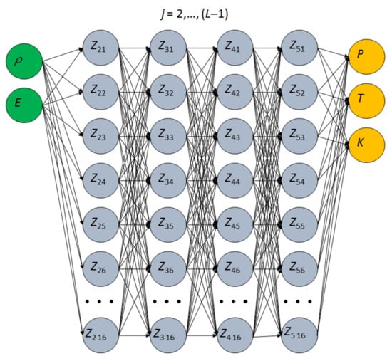
Figure 3.
Structure of the artificial neural network (ANN) for equation of state: 4 × 16 hidden layers, three inputs and six outputs; the neurons are ordered in layers, and the signals are transmitted in one direction–from the input layer toward the output one.
Sequential calculation of signals, Equation (25), from to allows one to find the output vector starting with the input one if the weights and biases are known.
The applied procedure of training is described in detail elsewhere [55,56]. It consists in sequential minimization of the approximation error by random variation of ANN parameters in the directions opposite to the corresponding gradient of the error over parameters. The gradient can be found through a set of matrix multiplications referred as the ‘backpropagation algorithm’. The choice of ANN structure is discussed in [56] for a more complex case of tensor equation of state. Here the approximated function is simpler, and to reduce the computation time in the following 3D modeling, we apply a simpler ANN with 16 neurons per layer as opposed to 64 neurons per layer used in [56]. This structure of the ANN allows us to obtain the average error of about 0.8% and the maximal error of about 5%; the comparison of the predictions of the trained ANN with the training data set from the MD is shown in Figure 4. Validation of the trained ANN is performed by comparison with MD data for intermediate temperatures of 350 K and 550 K. Similar to [56] the error on the testing data set is smaller than that on the training one; therefore, this procedure seems to be excessive for smooth data. The obtained parameters of the trained ANN are given in the Supplementary Materials, and the structure of the file is described in Appendix B. It allows one to use the developed equation of state by applying this file with weights and biases together with Equations (25)–(27) for processing of the signals of the ANN.
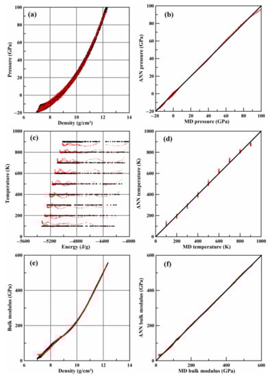
Figure 4.
The equation of state of copper: (a–c) ANN results (red crosses) in comparison with MD data of the training data set for (a) pressure, (c) temperature and (e) bulk modulus; (b,d,f) the corresponding correlation graphs, where the black line shows the ideal case.
2.4. Numerical Scheme of the Smoothed Particle Hydrodynamics (SPH)
The equations with spatial derivatives, such as Equations (1)–(3), (5) and (6), are numerically solved by using the approach of the SPH (smoothed particle hydrodynamics) [85,86,87]. Within this approach, the continuum medium is divided on the particles, and the mechanical characteristics of each particle are smudged around its center by using a smoothing kernel , where is the radius vector of the center of the particle, is the radius vector of the spatial point, where the characteristics are determined, is the linear scale of smoothing. The kernel should be normalized to 1, rapidly decreasing with the increase in and close to zero far from the particle, where . We apply the widely used kernel, which is based on the cubic spline [85]:
where is the dimensionless distance. A mechanical characteristic denoted as , which can be mass density, stresses or velocity, can be calculated in an arbitrary point in space through its values in the centers of the particles by using the following interpolation formula:
where and are the mass and mass density of b-th particle. The summation in Equation (29) is formally carried out over all particles, but due to the properties of the kernel function, Equation (28), only the nearest neighbors give a non-zero contribution to the sum. In order to ensure vanish of gradient on a constant field, the following form of the spatial derivatives at the position of the center of a-th particle is introduced [85]:
where the function follows from differentiation of the kernel, Equation (28), over :
Using this approach, the following approximations of the conservation laws of mass and momentum, Equations (1) and (2), can be written out:
where the sum in Equation (33) ensues the conservation of both angular and linear momentum [85,86], because it makes symmetrical the force acting on a-th particles from the side of b-th one and the opposite force, which acts on b-th particle from a-th one. The value represents the artificial viscosity, which provides stability of the numerical solution near the shock wave fronts. Following [86], we use a combined artificial viscosity, which includes both linear and quadratic ones:
where is the bulk sound speed; the value with the dimension of velocity is equal to zero for a couple of particles moving away from each other, and it is positive for the particles approaching each other:
The numerical scheme for the equation of internal energy, Equation (3), is adopted to provide the energy conservation in the couple with Equation (33):
It is shown in [41] that usage of physical viscosity instead of the artificial one can provide a stable numerical solution on a sufficiently fine numerical grid. This approach also gives a correct description of non-uniform temperature distributions in the form of high-entropy and low-entropy layers in the transition areas of shock wave formation and reflection. On the other hand, it is hard to provide the required mesh resolution in a 3D case; therefore, we use artificial viscosity in Equations (33) and (35).
In the case of elastic-plastic medium, we have to calculate velocity gradient , which enters Equation (5) for the macroscopic strain tensor and Equation (6) for the rotation tensor:
All other equations of the dislocation plasticity model are local. They describe processes in each particle separately and do not involve spatial derivatives. Integration in time of all equations is realized by explicit Euler scheme with the time step determined from the Courant–Friedrichs–Lewy condition:
The numerical solution in one-thread mode is implemented as FORTRAN program SPHEP (SPH for elastic-plastic flows). The time of calculation of the sums over particles determines the performance of the algorithm to the greatest extent. Only the nearest particles with the dimensionless distance smaller than 2 are taken into account during summation, because more distant particles give zero contribution. For fast searching of the neighbor particles, the computation domain is divided on rectangles with the sides nor less than . Only the particles in 27 (3 × 3 × 3) rectangles closest to the current particle including the one in which it is located, are tested to satisfy the condition . The SPH particles are initially placed in the sites of BCC lattice with a period equal to the linear scale of smoothing . This does not relate to the crystal structure of the material, but is only used for arrangement of SPH particles as discrete representatives of the medium. The BCC arrangement provides a better result including better connections between SPH particles than a simple cubic one. The number of SPH particles in the system reaches about 63 thousands. In the case of one-thread program, the optimization in computation time is achieved by running a set of calculations for different conditions of collision on dual-processor system (up to 40 threads) at once. Due to implementation of the complex plasticity model, the calculation time reaches 10 days on a single thread. Multithread parallel version of the program running on a CPU is considered in the following section.
2.5. Parallel Algorithm
We apply the Message Passing Interface (MPI) to speed up solving numerical problems on a multi-core processor. The multithread parallel version is written as C++ program MTHREAD_SPHEP. For distribution of particles between threads, we use the approach in which each process calculates a certain array of particles independent of their location in the substance, see Figure 5. Because the SPH particles with close numbers are initially situated in the same parts of solid samples, and there is no drastic change of neighbors, this approach seems to be reasonable for the problem under consideration.

Figure 5.
Scheme of smoothed particle hydrodynamics (SPH) particle distribution between processes in the parallel version of the algorithm.
The calculations are distributed between the processes as follows. At the beginning of the program, the initial distribution of particles and their thermodynamic characteristics are set by the master process. Then, the number of particles per each regular process is determined based on the total number of particles and the number of processes : , where the function returns the integer part of a floating point number. The number of particles processed by the last process is greater on , which is equal to the remainder of the division of by . The master process distributes arrays containing data on all particles to each one of the processes at the beginning of each simulation cycle and assigns the processes to calculate the corresponding particles. Thereafter, all processes simultaneously solve the system of equations containing conservation laws, calculate the deformations, stresses, and thermodynamic characteristics, and define new positions of their particles. Updated values are sent to the master process, which redistributes them for all processes as the initial state for calculation of the next time step. The master process also constitutes the neighbors list and writes data to the file. The data transfer is done for every time step, the neighbors list is updated every 10 time steps, while data are written in the file every 1000 time steps.
It is known that an increase in the number of computational processes in parallel computing does not mean a direct proportional increase in performance [88]. The speed-up factor characterizing acceleration of computations is determined by the ratio of the execution time of the sequential algorithm to the execution time of the parallel program [89]. The bottleneck is the portion of the code that cannot be solved in parallel, which principally restricts the speed-up factor. The efficiency of the algorithm is determined by the ratio of acceleration to the number of processes. The speed-up and efficiency of the developed parallel algorithm are shown in Figure 6 as functions of the number of processes. The real speed-up non-linearly falls behind the idealized linear growth. The program has a portion of operations that are solved sequentially: setting of initial conditions, generating a list of neighbors, and writing data to a file are performed in a non-parallel manner, which reduces the efficiency of the parallel algorithm. In addition, the decrease in efficiency is associated with an increase in the number of transfers between the processes. Meanwhile, the parallel algorithm substantially reduces the computation time in comparison with the sequential one. This is because the computation of gradients in SPH involving time-consuming cycles over neighboring particles, as well as processing of local variables for dislocation slip and calculation of the ANN for the equation of state, take more computation time than the data transfer and sequential parts of the algorithm.
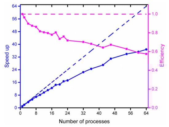
Figure 6.
Speed-up (the blue line and left scale) and efficiency (purple line and right scale) of the parallel algorithm as functions of the number of processes; dashed lines show ideal limit.
3. Results
3.1. Results of Experiments
In our experiments we register only the final form of the impacted specimens. In spite of the fact that most modern experimental setups for Taylor impact test are equipped with high-speed cameras, the comparison of the final form between experiment and modeling remains the widely used technique [16]. Photographs of the specimens impacted with different velocities are shown in Figure 7.

Figure 7.
Results of experiments: The final form of the deformed samples at different impact velocities in comparison with the reference one.
The raw data of experiments (initial and deformed lengths and diameters) are collected in Appendix A. The impact causes flattening of the part of the colliding edge of cylindrical samples; the impact velocity is higher, and the flattening is higher. The sample impacted at 113.6 m/s was initially shorter than the others in order to reduce its mass and increase the impact velocity, see Appendix A.
3.2. Microstructural Analysis
The following samples were selected for microstructural analysis of the material: (i) the cylinder impacted at 86.9 m/s, (ii) the shorter cylinder impacted at 113.6 m/s and (iii) undeformed cylinder.
The samples were placed in a container and filled with epoxy resin. Thereafter, they were manually micropolished using moisture-resistant sandpaper with a periodic cooling in water to avoid overheating of the samples and possible changes in the structure. A photo of the finished polished section is shown in Figure 8.
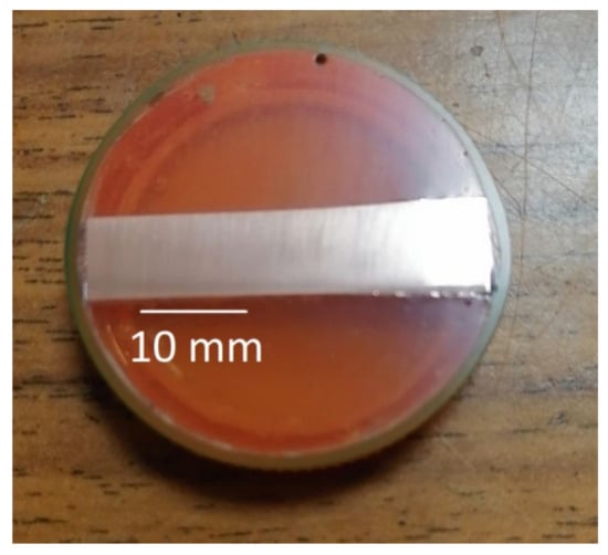
Figure 8.
Photo of the polished section before etching.
Etching of the samples was carried out using a solution of hydrogen peroxide 3%, citric acid and salt. In the undeformed part of the sample, the grains have a characteristic luster of metallic copper, impurities and oxides are not visualized. The grains are clearly elongated in the direction of rolling (axial direction) as shown in Figure 9A. The area method with several investigated samples gives the average grain diameter of about (17.5 ± 3.5) µm. Localization bands of plastic flow with the width of 15–20 µm are clearly visualized in the undeformed part of the sample. These bands go along the rolling direction of the copper rod and look like small depressions consisting mainly of small grains less than 2 µm in size as shown in Figure 9B,C. In the undeformed parts of the samples at high magnification (1000×), a subgrain mesh structure with the size of subgrain up to 3 µm can clearly be seen, see Figure 10. All these features reflect the microstructure resulting from the quasi-static deformation of cold rolling applied at the stage of manufacturing of the rods.
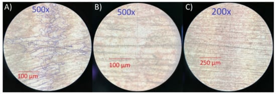
Figure 9.
Photo of the microstructure of an undeformed copper sample obtained using a metallographic microscope; (A) grains are schematically marked for size estimation by the area method; (B,C) localization bands of plastic flow with the characteristic size of 15–20 µm are seen.
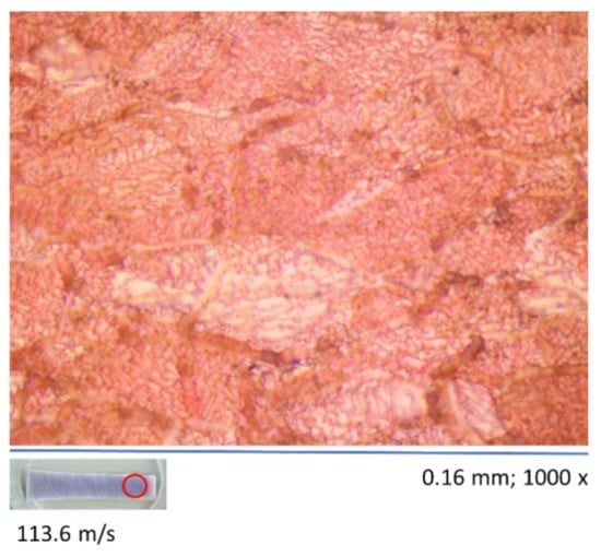
Figure 10.
Photo of the subgrain structure in the undeformed rear part of the sample: Magnification of 1000× is used.
In the dynamically deformed samples, a significant reduction in the grain sizes is observed. The final grain size is difficult to determine by means of the metallographic microscope used. Near the impact surface, the size of most of the grains can be estimated from above as less than 1 µm, while individual coarse grains are also visible with a diameter of about (16.5 ± 2.5) µm, which is close to that in the undeformed material. At a distance of 3 mm from the impact surface, conglomerates of reduced grains with an average diameter of about (7 ± 2) µm are observed with submicrometer grains at the boundary of these conglomerates. Grains in these conglomerates are equiaxial as opposed to the elongated grains in the raw material. The refinement and leveling of grain sizes along different directions are consequences of the dynamic deformation during the impact. Besides the refinement of grains, we detect near the impact surface a number of pores with the diameters of about 15–30 µm, Figure 11A,B,D and localization bands, Figure 11A,B. Although the presence of pore-like structures is not in doubt, we cannot distinguish between their occurrence during the dynamic impact or during the etching. We cannot eliminate the possibility that these pores are chemically etched in the weak areas of material (intersections of localization bands, for instance) during the slice preparation. If we consider the structure of the sample in areas of moderate plastic deformation (closer to the middle of the cylinder), then we can observe a mixed microstructure: ordinary grains similar in size to the grains in the undeformed sample with a fine-grained structure on the border between larger grains, Figure 11C.
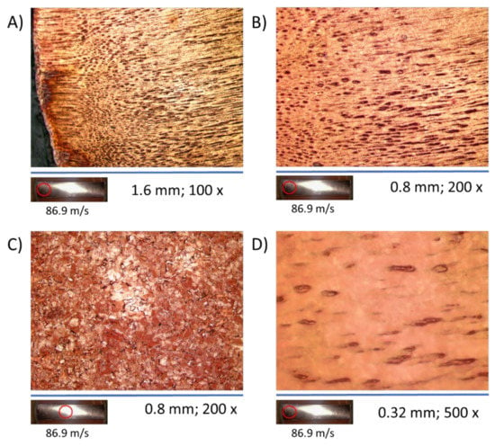
Figure 11.
Photos of the microstructure of deformed sample impacted with the velocity of 86.9 m/s: (A) near the impact surface, magnification is 100×; (B) near the impact surface, magnification is 200×; (C) combination of ultrafine-grained and fine-grained microstructure in the area of moderate plastic deformation near the center of the sample, magnification is 200×; (D) pores near the impact surface, magnification is 500×.
3.3. Results of Numerical Modeling in Comparison with Experiment
The numerical model used in 3D calculations is shown in Figure 12; the OVITO program [90] was used for visualization with each SPH particle represented by a small sphere. The number of SPH particles was chosen from a preliminary parametric study to provide a compromise between the precision and the duration of computations. Free boundary conditions were set along all the surfaces of the projectile except the contact with the anvil, which is impenetrable and with free sliding. The initial velocity directed to the anvil was set for all SPH particles. We compared the results of modeling with experimental data on final shapes, sizes and deformations of the impacted samples, and analyzed the impact conditions basing on the modeling results.

Figure 12.
Three-dimensional (3D) numerical model of the impacted specimen: The number of SPH particles is equal to 63,125.
Figure 13 compares the modeling and experimental results. The modeling repeats the experimental tendency of shortening of the specimens. The degree of shortening increases together with the increase in impact velocity similarly in both experiment and modeling. The deformation is close to axisymmetric, while an uneven increase in diameter can be seen for some experimental samples: the impact surface looks like an ellipse.

Figure 13.
The final shape of the specimens with various impact velocities: comparison of the experimental data and the modeling results.
Figure 14 shows the spatial distribution of the von Mises equivalent stress which is calculated through the stress deviator as follows:
and equal to the flow stress in the case of simple tension or compression. The modeling results in Figure 14 are for the highest impact velocity in experiment for the samples with the initial length of 40 mm. One can see a close to uniform field of the von Mises stress of about 0.5 GPa propagating along the cylinder—this is the area of plastic flow. The stress attenuates after the stopping of the projectile and the beginning of its reflection.
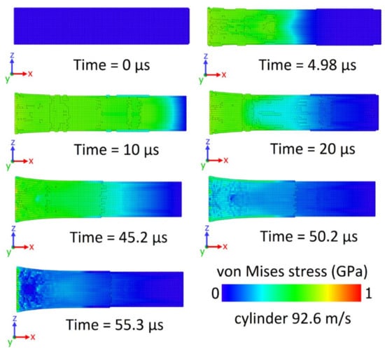
Figure 14.
Spatial distribution of the von Mises equivalent stress in subsequent moments of time: the impact velocity is 92.6 m/s.
Figure 15 shows the von Mises equivalent plastic strain , which is a scalar measure of the plastic strain tensor :

Figure 15.
Spatial distribution of the von Mises equivalent strain in subsequent moments of time: the impact velocity is 92.6 m/s.
Plastic deformation is concentrated near the impact surface and quickly attenuates with the distance from this surface. Plastic deformation in the center of the contact surface takes the greatest values. This is explained by the following: if we consider two lines, for example, drawn through rows of SPH particles, one in the center and the other on the periphery, the central line shortens during deformation, while the peripheral line bends, but retains a longer length. In other words, the shell is stretched on the shortening core of the impacted part of the cylinder. The region of the greatest plastic deformation agrees well with the microstructural analysis of the sample impacted at the velocity of 86.9 m/s presented in Figure 11. The largest number of pores is observed near the impact plane in the center of the sample and the largest values of plastic deformations in the numerical experiment are observed in the same place. It indicates the coincidence of the numerical experiment with the microstructural analysis of copper impactors.
Substantial influence of thermal softening is discussed in [30] for the case of OFHC copper. Figure 16 shows that the temperature increment does not exceed 170 K even in the central part of the head cylinder for the considered impact velocities.
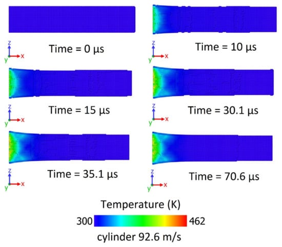
Figure 16.
Spatial distribution of the temperature in subsequent moments of time: the impact velocity is 92.6 m/s.
Figure 17 shows the radial strains calculated during simulation and measured in experiments. One can see a good correlation between numerical and experimental results, which indicates the applicability of the developed model and its numerical implementation. Thus, the model can be used to study the deformation conditions of the material during the impact test. Appendix A compares the initial experimental data, such as diameters and lengths, with the corresponding values obtained as a result of modeling. We chose the Green–Lagrangian strain tensor component:
where and are the initial and final diameters of the impact edge of the cylinder.

Figure 17.
Calculated radial strains in comparison with the experimental ones: Taylor impact tests for 8 mm OHFC copper rods.
Figure 18 shows the calculated radial strain rate for the sample colliding with an obstacle at a velocity of 92.6 m/s. At the beginning of the deformation, the strain rate reaches a peak value of about 1.7 × 10⁴ s−1, then monotonically decreases until the sample stops, and the stopping time is approximately 43 µs.
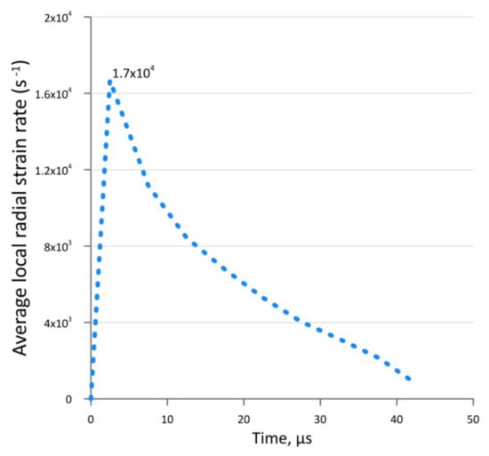
Figure 18.
Time dependence of the radial strain rate at the impact surface for the impact velocity of 92.6 m/s.
3.4. Determination of Optimal Coefficients for the Numerical Scheme of Elastic-Plastic Deformations
The model coefficients used in the previous section and listed in Table 1 are changed compared to the original source [43], where these parameters are fitted to the case of a copper single crystal. The initial density of immobilized dislocations is increased to the level of 1013 m−2, which is typical for the deformed metals. The change in the initial density of immobilized dislocations is due to the fine-grained structure of the initial state of the sample material shown by the performed microstructural analysis. The fine-grained structure is due to the method of production of the rods, which are used for the preparation of the samples. These rods were obtained by cold-rolling, which causes the growth of dislocation density and the appearance of subgrain conglomerates. It is known that, in turn, hot-rolled copper has a coarse-grained structure and lower dislocation density. Therefore, in order to match the experimental data, we increase the density of immobilized dislocations. The initial state of material can also influence the strain hardening.
The experimental data obtained are used to fit the hardening coefficient . We vary this coefficient in the range from 1 to 6 to select adequate values of hardening and good compliance with the experimental data. Figure 19 shows the dependence of the decrement of the sample length on the impact velocity, while Figure 20 shows the dependence of the diameter increment on the impact velocity. The experimental data are plotted together with the numerical dependencies obtained at different values of the hardening coefficient. Based on the obtained results, we chose the hardening coefficient as a compromise allowing us to describe the change in both length and diameter simultaneously.
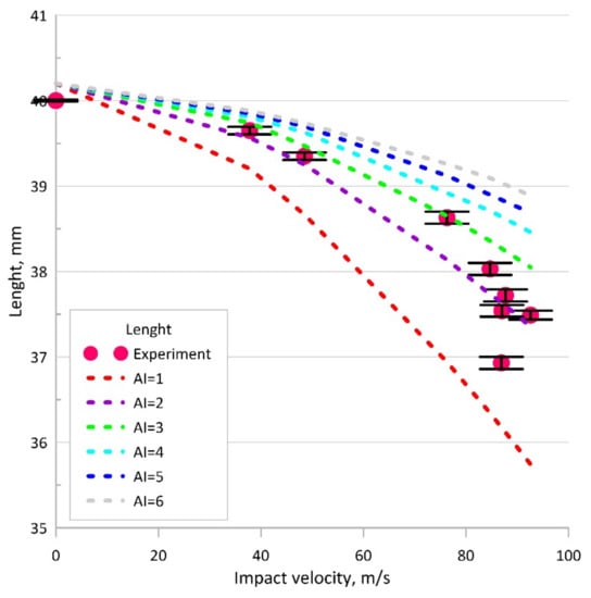
Figure 19.
Quantitative comparison of modeling and experiments for various hardening coefficients: The dependence of the final length after deformation on the impact velocity; the dashed lines present the results of numerical modeling.
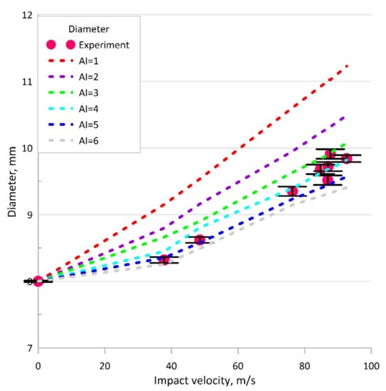
Figure 20.
Quantitative comparison of modeling and experiments for various hardening coefficients: The dependence of the final diameter after deformation on the impact velocity; the dashed lines present the results of numerical modeling.
4. Discussion
We develop a combined experimental-numerical approach to study the dynamic plasticity of metals and apply it to OFHC copper. A combination of experiments with analytical consideration [31,32,33,91] or numerical modeling [16,92,93] is known to be a fruitful approach to the investigation of dynamic plasticity and fracture of various materials. In the experimental part, the Taylor impact tests with cold-rolled OFHC copper allowed us to achieve large plastic deformation with the strain rate up to 1.7 × 10⁴ s−1 at the impact velocity below 100 m/s. With an increase in the impact velocity, a monotonous increase in the diameter and a decrease in the length of the sample were observed.
Microstructural analysis revealed that these copper samples initially had a fine-grained structure with an average grain diameter of (17.5 ± 3.5) µm. Localization bands with a characteristic width of 15–20 µm were visualized in an undeformed sample; these localization bands represented areas of concentration of submicron grains. The appearance of localization bands in undeformed samples is caused by the method of manufacturing of the copper rods—cold pressing and subsequent stretching. Bending of the localization bands and formation of pore-like structures were observed in the dynamically deformed parts of the samples near the impact surface. We assume that the localization bands were involved in the process of pore formation during the dynamic deformation. Localization bands are the areas of “weak” material, which in combination with the stress concentration in these areas during dynamic deformation contributes to local destruction of the material. Also, it cannot be ruled out that temperature rise and possible recrystallization processes at the boundaries of localization bands are possible in the localization areas. This fact can also partially explain the pore formation. Subgrain structure with an average subgrain size of up to 2 μm was visualized in the undeformed parts of the samples. The sub-grains were not separate conglomerates at the grain boundaries, but had a structure in the form of a mesh over the entire material, visualized over large areas of the grain structure. This structure is characteristic of metals subjected to large plastic deformations, which is explained by pressing the metal during its manufacture. In general, the dynamic deformation during the Taylor impact test led to further refinement of the grain structure, bending of the localization bands and formation of pore-like structures in the most deformed parts of the samples near the impact surface. Besides this, the grains in the dynamically deformed parts of sample became equiaxial in contrast to elongated grains of the initial cold-rolled material.
In terms of modeling, the dislocation plasticity model, previously tested for the shock wave problem at plate impact [39,43,44], was implemented in 3D using the numerical scheme of smoothed particle hydrodynamics (SPH). The model includes an equation of state implemented in the form of an artificial neural network (ANN) and trained according to MD simulations of uniform isothermal stretching/compression of representative volumes of copper; the equation of state is also used to calculate the shear modulus. Currently, ANNs are widely used in materials science [94,95,96]. In the present research, application of the ANN was more of a methodological issue, because there are a number of reliable equations of state for pure copper. The development of this methodology was reasonable in view of the prospects to approximate stress tensor instead of scalar pressure and for application to new materials including metal alloys, high-entropy alloys, etc. The dislocation friction coefficient in copper obtained in [76] as a result of MD modeling was used. These two efforts were aimed at construction of a fully MD-based model of material, which should require only experimental verification, but not parameter identification. A future step will be the parametrization of the dislocation kinetics submodel. In this study the corresponding parameters were partially used from a previous study [43], where they were determined by comparison with experimental results on plate impacts, and partially selected to fit the numerical results to the present experimental data—in this way we selected the hardening parameter. Comparison of the final shape of the projectile, values of shortening, and radial strain confirmed the applicability of the developed numerical model.
Future development of the present approach to modeling will be associated with explicit consideration of the formalism of large deformations [97,98] and the construction of a complete tensor equation of state connecting the elastic strain tensor with the stress tensor using MD-informed ANN [99]. It is also possible to add a material fracture model to compare pore densities with microstructural analysis. The development of the experimental program involves application to other metals and alloys, the study of the effect of the initial state of the defective system (annealing and thermomechanical processing, which will minimize or completely eliminate the presence of localization bands) on the dynamic shear strength, as well as testing various shapes of similar-sized samples (cone, ball, truncated cylinder) to increase stresses in the collision region, which would allow large deformations to be achieved at comparable impact velocities and increase the strain rate.
5. Conclusions
In this paper, we applied a combined experimental-numerical approach to study the dynamic plasticity of cold-rolled OFHC copper. In the experimental part, impact velocities up to 113.6 m/s provided a strain up to 0.3 and strain rates up to 1.7 × 10⁴ s−1 at the edge of the sample. Microstructural analysis showed pore-like structures with sizes of about 15–30 µm and significant refinement of the grain structure in the deformed parts of the sample with the formation of submicron grains. The dislocation plasticity model was implemented in the 3D case using the numerical scheme of smoothed particle hydrodynamics (SPH). The model includes an equation of state in the form of an artificial neural network and trained according to MD simulations of uniform isothermal stretching/compression of representative volumes of copper. Comparison with the experiment confirmed the applicability of the developed numerical model and allowed us to optimize the model parameters for the case of cold-rolled OFHC copper.
Supplementary Materials
The following supporting information can be downloaded at: https://www.mdpi.com/article/10.3390/met12020264/s1, File Cu.EOS.ANNp.xlsx: file with parameters of ANN for equation of state of copper.
Author Contributions
Conceptualization, A.E.M., P.N.M. and E.S.R.; methodology, E.S.R. and V.G.L.; software, A.E.M., P.N.M., N.A.G. and E.S.R.; validation, E.S.R. and N.A.G.; formal analysis, E.S.R.; investigation, E.S.R. and V.G.L.; resources, P.N.M.; data curation, E.S.R.; writing—original draft preparation, A.E.M., P.N.M., N.A.G. and E.S.R.; writing—review and editing, A.E.M.; visualization, E.S.R.; supervision, A.E.M.; project administration, P.N.M.; funding acquisition, P.N.M. All authors have read and agreed to the published version of the manuscript.
Funding
This research and the APC were funded by the RUSSIAN SCIENCE FOUNDATION, grant number 20-79-10229.
Institutional Review Board Statement
Not applicable.
Informed Consent Statement
Not applicable.
Data Availability Statement
The raw data of experiments in comparison with numerical simulations are available in Appendix A. The equation of state in the form of parameter file of trained ANN is available as Supplementary Materials; the structure of this file is described in Appendix B.
Conflicts of Interest
The authors declare no conflict of interest.
Appendix A. Raw Data of Experiment in Comparison with Modeling
Table A1.
Experimental data in comparison with modeling for cylinders: initial and final length of the samples and diameter of the impacted edge of the samples.
Table A1.
Experimental data in comparison with modeling for cylinders: initial and final length of the samples and diameter of the impacted edge of the samples.
| Impact Velocity (m/s) | Initial Length (mm) | Final Length (mm) | Initial Diameter (mm) | Final Diameter (mm) | ||||
|---|---|---|---|---|---|---|---|---|
| Experiment | Model | Experiment | Model | Experiment | Model | Experiment | Model | |
| 37.8 | 40.0 | 40.2 | 39.65 | 39.207 | 8.00 | 8.00 | 8.32 | 8.738 |
| 48.5 | 39.35 | 38.693 | 8.62 | 8.928 | ||||
| 76.3 | 38.63 | 37.114 | 9.35 | 9.475 | ||||
| 84.7 | 38.03 | 36.586 | 9.68 | 9.646 | ||||
| 86.9 | 36.93 | 36.445 | 9.516 | 9.693 | ||||
| 87 | 37.54 | 36.439 | 9.72 | 9.693 | ||||
| 87.7 | 37.72 | 36.394 | 9.91 | 9.703 | ||||
| 92.6 | 37.49 | 36.078 | 9.84 | 9.805 | ||||
| 113.6 | 31.3 | 31.4 | 28.75 | 27.249 | 9.683 | 10.195 | ||
Appendix B. Structure of File with Parameters of ANN for Equation of State
The parameters of the trained ANN are attached as Supplementary Materials to this paper, which allows their use. The description of ANN parameter files are in Table A2. The structure of the file is as follows. The first line contains the number of layers . The second line contains the numbers of neurons in each layer printed sequentially: . The type of transfer function is not explicitly specified in the files, but ‘Leaky ReLU’ transfer function, Equation (27), is used for hidden layers and ‘Sigmoid’ transfer function, Equation (28), is used for the output layer. The third line should be missed. The weights are printed starting from the fourth line in the following order: , , …, ; line feed; , , …, ; line feed; …, ; empty line; , , , …, ; line feed; , , …, ; line feed; …, ; empty line, etcetera. The next line after the ending of the weight section should be missed. Following, the biases are printed in a similar order: , , …, ; empty line; , , …, ; empty line, etcetera. The next line after the ending of the bias section should be missed. The following lines contain minimal and maximal values for ANN inputs and outputs. All the input values before using in ANN should be normalized as . On the other hand, all the outputs should be restored as .
Table A2.
Description of ANN parameter file “Cu.EOS.ANNp”.
Table A2.
Description of ANN parameter file “Cu.EOS.ANNp”.
| Parameter | Value |
|---|---|
| Number of inputs | 2 |
| Inputs | |
| Number of outputs | 3 |
| Outputs |
References
- Kanel, G.I.; Razorenov, S.V.; Baumung, K.; Singer, J. Dynamic yield and tensile strength of aluminum single crystals at temperatures up to the melting point. J. Appl. Phys. 2001, 90, 136–143. [Google Scholar] [CrossRef]
- Winey, J.M.; LaLone, B.M.; Trivedi, P.B.; Gupta, Y.M. Elastic wave amplitudes in shock-com- pressed thin polycrystalline aluminum samples. J. Appl. Phys. 2009, 106, 073508. [Google Scholar] [CrossRef]
- Gurrutxaga-Lerma, B.; Shehadeh, M.A.; Balint, D.S.; Dini, D.; Chen, L.; Eakins, D.E. The effect of temperature on the elastic precursor decay in shock loaded FCC aluminium and BCC iron. Int. J. Plast. 2017, 96, 135–155. [Google Scholar] [CrossRef]
- Saveleva, N.V.; Bayandin, Y.V.; Savinykh, A.S.; Garkushin, G.V.; Razorenov, S.V.; Naimark, O.B. The formation of elastoplastic fronts and spall fracture in amg6 alloy under shock-wave loading. Tech. Phys. Lett. 2018, 44, 823–826. [Google Scholar] [CrossRef]
- Gnyusov, S.F.; Rotshtein, V.P.; Mayer, A.E.; Rostov, V.V.; Gunin, A.V.; Khishchenko, K.V.; Levashov, P.R. Simulation and experimental investigation of the spall fracture of 304L stainless steel irradiated by a nanosecond relativistic high-current electron beam. Int. J. Fract. 2016, 199, 59–70. [Google Scholar] [CrossRef]
- Gnyusov, S.F.; Rotshtein, V.P.; Mayer, A.E.; Astafurova, E.G.; Rostov, V.V.; Gunin, A.V.; Maier, G.G. Comparative study of shock-wave hardening and substructure evolution of 304L and Hadfield steels irradiated with a nanosecond relativistic high-current electron beam. J. Alloys Compd. 2017, 714, 232–244. [Google Scholar] [CrossRef]
- Baumung, K.; Bluhm, H.J.; Goel, B.; Hoppé, P.; Karow, H.U.; Rusch, D.; Fortov, V.E.; Kanel, G.I.; Razorenov, S.V.; Utkin, A.V.; et al. Shock-wave physics exper- iments with high-power proton beams. Laser Part Beams 1996, 14, 181–209. [Google Scholar] [CrossRef]
- Baumung, K.; Bluhm, H.; Kanel, G.I.; Müller, G.; Razorenov, S.V.; Singer, J.; Utkin, A.V. Tensile strength of five metals and alloys in the nanosecond load duration range at normal and elevated temperatures. Int. J. Impact. Eng. 2001, 25, 631–639. [Google Scholar] [CrossRef]
- Moshe, E.; Eliezer, S.; Dekel, E.; Ludmirsky, A.; Henis, Z.; Werdiger, M.; Goldberg, I.B. An increase of the spall strength in aluminum, copper, and Metglas at strain rates larger than 107 s−1. J. Appl. Phys. 1998, 83, 4004. [Google Scholar] [CrossRef] [Green Version]
- Krasyuk, I.K.; Pashinin, P.P.; Semenov, A.Y.; Khishchenko, K.V.; Fortov, V.E. Study of extreme states of matter at high energy densities and high strain rates with powerful lasers. Laser Phys. 2016, 26, 094001. [Google Scholar] [CrossRef] [Green Version]
- Ashitkov, S.I.; Komarov, P.S.; Struleva, E.V.; Agranat, M.B.; Kanel, G.I. Mechanical and optical properties of vanadium under shock picosecond loads. JETP Lett. 2015, 101, 276–281. [Google Scholar] [CrossRef]
- Kanel, G.I.; Zaretsky, E.B.; Razorenov, S.V.; Ashitkov, S.I.; Fortov, V.E. Unusual plasticity and strength of metals at ultra-short load durations. Phys. Usp. 2017, 60, 490–508. [Google Scholar] [CrossRef] [Green Version]
- Zuanetti, B.; McGrane, S.D.; Bolme, C.A.; Prakash, V. Measurement of elastic precursor decay in pre-heated aluminum films under ultra-fast laser generated shocks. J. Appl. Phys. 2018, 123, 195104. [Google Scholar] [CrossRef] [Green Version]
- Bilalov, D.A.; Sokovikov, M.A.; Chudinov, V.V.; Oborin, V.A.; Bayandin, Y.V.; Terekhina, A.I.; Naimark, O.B. Numerical simulation and experimental study of plastic strain lo- calization under the dynamic loading of specimens in conditions close to a pure shear. J. Appl. Mech. Tech. Phys. 2018, 59, 1179–1188. [Google Scholar] [CrossRef]
- Nie, H.; Suo, T.; Wu, B.; Li, Y.; Zhao, H. A versatile split Hopkinson pressure bar using electromagnetic loading. Int. J. Impact Eng. 2018, 116, 94–104. [Google Scholar] [CrossRef]
- Nguyen, T.; Fensin, S.J.; Luscher, D.J. Dynamic crystal plasticity modeling of single crystal tantalum and validation using Taylor cylinder impact tests. Int. J. Plast. 2021, 139, 102940. [Google Scholar] [CrossRef]
- Grässel, O.; Krüger, L.; Frommeyer, G.; Meyer, L.W. High strength Fe-Mn-(Al, Si) TRIP/TWIP steels development–properties–application. Int. J. Plast. 2000, 16, 1391–1409. [Google Scholar] [CrossRef]
- Taylor, G.I. The use of flat-ended projectiles for determining dynamic yield stress. I. Theoretical considerations. Proc. R. Soc. Lond. Ser. A 1948, 194, 289–299. [Google Scholar] [CrossRef]
- Whiffin, A.C. The use of flat-ended projectiles for determining dynamic yield stress. II. Tests on various metallic materials. Proc. R. Soc. Lond. Ser. A 1948, 194, 300–322. [Google Scholar] [CrossRef] [Green Version]
- Carrington, W.E.; Gayler, M.L.V. The use of flat-ended projectiles for determining dynamic yield stress III. Changes in microstructure caused by deformation under impact at high-striking velocities. Proc. R. Soc. Lond. Ser. A 1948, 194, 323–331. [Google Scholar] [CrossRef] [Green Version]
- Khayer Dastjerdi, A.; Naghdabadi, R.; Arghavani, J. An energy-based approach for analysis of dynamic plastic deformation of metals. Int. J. Mech. Sci. 2013, 66, 94–100. [Google Scholar] [CrossRef]
- Gao, C.; Iwamoto, T. Finite element analysis on a newly-modified method for the Taylor impact test to measure the stress-strain curve by the only single test using pure aluminum. Metals 2018, 8, 642. [Google Scholar] [CrossRef] [Green Version]
- Rakvåg, K.G.; Børvik, T.; Westermann, I.; Hopperstad, O.S. An experimental study on the deformation and fracture modes of steel projectiles during impact. Mater. Des. 2013, 51, 242–256. [Google Scholar] [CrossRef] [Green Version]
- Borodin, E.N.; Mayer, A.E. Structural model of mechanical twinning and its application for modeling of the severe plastic deformation of copper rods in Taylor impact tests. Int. J. Plast. 2015, 74, 141–157. [Google Scholar] [CrossRef]
- Volkov, G.A.; Bratov, V.A.; Borodin, E.N.; Evstifeev, A.D.; Mikhailova, N.V. Numerical simulations of impact Taylor tests. J. Phys. Conf. Ser. 2020, 1556, 012059. [Google Scholar] [CrossRef]
- Zhang, L.; Pellegrino, A.; Townsend, D.; Petrinic, N. Thermomechanical constitutive behaviour of a near 𝛼 titanium alloy over a wide range of strain rates: Experiments and modelling. Int. J. Mech. Sci. 2021, 189, 105970. [Google Scholar] [CrossRef]
- Rakvåg, K.G.; Børvik, T.; Hopperstad, O.S. A numerical study on the deformation and fracture modes of steel projectiles during Taylor bar impact tests. Int. J. Solids Struct. 2014, 51, 808–821. [Google Scholar] [CrossRef] [Green Version]
- Moćko, W.; Janiszewski, J.; Radziejewska, J.; Gra¸zka, M. Analysis of deformation history and damage initiation for 6082-T6 aluminium alloy loaded at classic and symmetric Taylor impact test conditions. Int. J. Impact. Eng. 2015, 75, 203–213. [Google Scholar] [CrossRef]
- Xiao, X.; Mu, Z.; Pan, H.; Lou, Y. Effect of the Lode parameter in predicting shear cracking of 2024-T351 aluminum alloy Taylor rods. Int. J. Impact. Eng. 2018, 120, 185–201. [Google Scholar] [CrossRef]
- Piao, M.J.; Huh, H.; Lee, I.; Park, L. Characterization of hardening behaviors of 4130 Steel, OFHC Copper, Ti6Al4V alloy considering ultra-high strain rates and high temperatures. Int. J. Mech. Sci. 2017, 131, 1117–1129. [Google Scholar] [CrossRef]
- Kanel, G.I.; Savinykh, A.S.; Garkushin, G.V.; Razorenov, S.V. Effects of temperature on the flow stress of aluminum in shock waves and rarefaction waves. J. Appl. Phys. 2020, 127, 035901. [Google Scholar] [CrossRef]
- Zaretsky, E.B.; Kanel, G.I. Response of copper to shock-wave loading at temperatures up to the melting point. J. Appl. Phys. 2013, 114, 083511. [Google Scholar] [CrossRef]
- Kanel, G.I.; Savinykh, A.S.; Garkushin, G.V.; Razorenov, S.V. Effects of temperature and strain on the resistance to high-rate deformation of copper in shock waves. J. Appl. Phys. 2020, 128, 115901. [Google Scholar] [CrossRef]
- Kuksin, A.Y.; Stegailov, V.V.; Yanilkin, A.V. Molecular-dynamics simulation of edge-dislocation dynamics in aluminum. Dokl. Phys. 2008, 53, 287–291. [Google Scholar] [CrossRef]
- Krasnikov, V.S.; Kuksin, A.Y.; Mayer, A.E.; Yanilkin, A.V. Plastic deformation under high-rate loading: The multiscale approach. Phys. Solid State 2010, 52, 1386–1396. [Google Scholar] [CrossRef]
- Krasnikov, V.S.; Mayer, A.E. Influence of local stresses on motion of edge dislocation in aluminum. Int. J. Plast. 2018, 101, 170–187. [Google Scholar] [CrossRef]
- Austin, R.A.; McDowell, D.L. A dislocation-based constitutive model for viscoplastic deformation of fcc metals at very high strain rates. Int. J. Plast. 2011, 27, 1–24. [Google Scholar] [CrossRef]
- Barton, N.R.; Bernier, J.V.; Becker, R.; Arsenlis, A.; Cavallo, R.; Marian, J.; Rhee, M.; Park, H.-S.; Remington, B.A.; Olson, R.T. A multiscale strength model for extreme loading conditions. J. Appl. Phys. 2011, 109, 073501. [Google Scholar] [CrossRef]
- Krasnikov, V.S.; Mayer, A.E.; Yalovets, A.P. Dislocation based high-rate plasticity model and its application to plate-impact and ultra-short electron irradiation simulations. Int. J. Plast. 2011, 27, 1294–1308. [Google Scholar] [CrossRef]
- Luscher, D.J.; Mayeur, J.R.; Mourad, H.M.; Hunter, A.; Kenamond, M.A. Coupling continuum dislocation transport with crystal plasticity for application to shock loading conditions. Int. J. Plast. 2016, 76, 111–129. [Google Scholar] [CrossRef] [Green Version]
- Khishchenko, K.V.; Mayer, A.E. High- and low-entropy layers in solids behind shock and ramp compression waves. Int. J. Mech. Sci. 2021, 189, 105971. [Google Scholar] [CrossRef]
- Lim, H.; Carroll, J.D.; Battaile, C.C.; Chen, S.R.; Moore, A.P.; Lane, J.M.D. Anisotropy and strain localization in dynamic impact experiments of tantalum single crystals. Sci. Rep. 2018, 8, 5540. [Google Scholar] [CrossRef] [Green Version]
- Mayer, A.E.; Khishchenko, K.V.; Levashov, P.R.; Mayer, P.N. Modeling of plasticity and fracture of metals at shock loading. J. Appl. Phys. 2013, 113, 93508. [Google Scholar] [CrossRef]
- Yao, S.L.; Pei, X.Y.; Yu, J.D.; Bai, J.S.; Wu, Q. A dislocation-based explanation of quasi-elastic release in shock-loaded aluminum. J. Appl. Phys. 2017, 121, 035101. [Google Scholar] [CrossRef] [Green Version]
- Yao, S.; Pei, X.; Yu, J.; Wu, Q. Scale dependence of thermal hardening of fcc metals under shock loading. J. Appl. Phys. 2020, 128, 0026226. [Google Scholar] [CrossRef]
- Popova, T.V.; Mayer, A.E.; Khishchenko, K.V. Evolution of shock compression pulses in polymethylmethacrylate and aluminum. J. Appl. Phys. 2018, 123, 235902. [Google Scholar] [CrossRef]
- Selyutina, N.; Borodin, E.N.; Petrov, Y.; Mayer, A.E. The definition of characteristic times of plastic relaxation by dislocation slip and grain boundary sliding in copper and nickel. Int. J. Plast. 2016, 82, 97–111. [Google Scholar] [CrossRef]
- Gingold, R.A.; Monaghan, J.J. Smoothed particle hydrodynamics: Theory and application to non-spherical stars. Mon. Not. R. Astron. Soc. 1977, 181, 375–389. [Google Scholar] [CrossRef]
- Pan, W.; Li, D.; Tartakovsky, A.M.; Ahzi, S.; Khraisheh, M.; Khaleel, M. A new smoothed particle hydrodynamics non-Newtonian model for friction stir welding: Process modeling and simulation of microstructure evolution in a magnesium alloy. Int. J. Plast. 2013, 48, 189–204. [Google Scholar] [CrossRef]
- Li, X.; Roth, C.C.; Mohr, D. Machine-learning based temperature- and rate-dependent plasticity model: Application to analysis of fracture experiments on DP steel. Int. J. Plast. 2019, 118, 320–344. [Google Scholar] [CrossRef]
- Islam, M.R.I.; Chakraborty, S.; Shaw, A. On consistency and energy conservation in smoothed particle hydrodynamics. Int. J. Numer. Methods Eng. 2018, 116, 601–632. [Google Scholar] [CrossRef]
- Jordan, B.; Gorji, M.B.; Mohr, D. Neural network model describing the temperature- and rate-dependent stress-strain response of polypropylene. Int. J. Plast. 2020, 135, 102811. [Google Scholar] [CrossRef]
- Gorji, M.B.; Mozaffar, M.; Heidenreich, J.N.; Cao, J.; Mohr, D. On the potential of recurrent neural networks for modeling path dependent plasticity. J. Mech. Phys. Solids 2020, 43, 103972. [Google Scholar] [CrossRef]
- Bonatti, C.; Mohr, D. Neural network model predicting forming limits for Bi-linear strain paths. Int. J. Plast. 2021, 137, 102886. [Google Scholar] [CrossRef]
- Grachyova, N.A.; Lekanov, M.V.; Mayer, A.E.; Fomin, E.V. Application of neural networks for modeling shock-wave processes in aluminum. Mech. Solids 2021, 56, 326–342. [Google Scholar] [CrossRef]
- Mayer, A.E.; Krasnikov, V.S.; Pogorelko, V.V. Dislocation nucleation in Al single crystal at shear parallel to (111) plane: Molecular dynamics simulations and nucleation theory with artificial neural networks. Int. J. Plast. 2021, 139, 102953. [Google Scholar] [CrossRef]
- Fortov, V.E.; Khishchenko, K.V.; Levashov, P.R.; Lomonosov, I.V. Wide-range multi-phase equations of state for metals. Nucl. Instrum. Methods Phys. Res. A 1998, 415, 604–608. [Google Scholar] [CrossRef]
- Borodin, E.N.; Mayer, A.E. Localization of plastic flow at dynamic channel angular pressing. Tech. Phys. 2013, 58, 1159–1163. [Google Scholar] [CrossRef]
- Mayer, A.E.; Borodin, E.N.; Mayer, P.N. Localization of plastic flow at high-rate simple shear. Int. J. Plast. 2013, 51, 188–199. [Google Scholar] [CrossRef]
- Krasnikov, V.S.; Mayer, A.E. Modeling of plastic localization in aluminum and Al–Cu alloys under shock loading. Mater. Sci. Eng. A 2014, 619, 354–363. [Google Scholar] [CrossRef]
- Bai, Y.; Dodd, B. Shear Localization: Occurrence Theories and Applications; Pergamon Press: Oxford, UK, 1992. [Google Scholar]
- Wright, T. The Physics and Mathematics of Adiabatic Shear Bands; Cambridge University Press: Cambridge, UK, 2002. [Google Scholar]
- Walley, S.M. Shear localization: A historical overview. Metall. Mater. Trans. A 2007, 38, 2629–2654. [Google Scholar] [CrossRef]
- Shockey, D.A.; Murr, L.E.; Staudhammer, K.P.; Meyers, M.A. (Eds.) Metallurgical Applications of Shock-Wave and High-Strain-Rate Phenomena; Marcel-Dekker: New York, NY, USA, 1986; pp. 633–656. [Google Scholar]
- Shahan, A.R.; Taheri, A.K. Adiabatic shear bands in titanium and titanium alloys: A critical review. Mater. Res. Bull. 1993, 14, 243–250. [Google Scholar] [CrossRef]
- Xu, Y.; Zhang, J.; Bai, Y.; Meyers, M.A. Shear localization in dynamic deformation: Microstructural evolution. Metall. Mater. Trans. A 2008, 39, 811–843. [Google Scholar] [CrossRef]
- Tresca, H. On further application of the flow of solids. Proc. Inst. Mech. Eng. 1878, 30, 301–345. [Google Scholar] [CrossRef]
- Massey, H.F. The flow of metals during forging. Trans. Manch. Eng. Assoc. 1921, 21–66. [Google Scholar]
- Johnson, W.; Baraya, G.L.; Slater, R.A.C. On heat lines or lines of thermal discontinuity. Int. J. Mech. Sci. 1964, 6, 409–414. [Google Scholar] [CrossRef]
- Zener, C.; Hollomon, J.H. Effect of strain rate upon plastic flow of steel. J. Appl. Phys. 1944, 15, 22–32. [Google Scholar] [CrossRef]
- Kuropatenko, V.F. New models of continuum mechanics. J. Eng. Phys. Thermophys. 2011, 84, 77–99. [Google Scholar] [CrossRef]
- Mayer, A.E.; Krasnikov, V.S.; Pogorelko, V.V. Homogeneous nucleation of dislocations in copper: Theory and approximate description based on molecular dynamics and artificial neural networks. 2022; submitted. [Google Scholar]
- Landau, L.D.; Lifshitz, E.M. Theory of Elasticity. Course of Theoretical Physics, 7; Pergamon: New York, NY, USA, 1986. [Google Scholar]
- Hirth, J.P.; Lothe, J. Theory of Dislocations; Wiley & Sons: New York, NY, USA, 1982. [Google Scholar]
- Dudorov, A.E.; Mayer, A.E. The equations of the dynamics and kinetics of dislocations at high strain rate plastic deformation. CSU Bull. Phys. 2011, 39, 48–56. (In Russian) [Google Scholar]
- Mayer, A.E.; Krasnikov, V.S. Molecular dynamics investigation of dislocation slip in pure metals and alloys. In Proceedings of the Second International Conference on Theoretical, Applied and Experimental Mechanics, ICTAEM 2019, Corfu, Greece, 23–26 June 2019; Volume 8, pp. 59–64. [Google Scholar] [CrossRef]
- Franciosi, P. The concepts of latent hardening and strain hardening in metallic single crystals. Acta Metall. 1985, 33, 1601–1612. [Google Scholar] [CrossRef]
- Devincre, B.; Kubin, L.; Hoc, T. Physical analyses of crystal plasticity by DD simulations. Scr. Mater. 2006, 54, 741–746. [Google Scholar] [CrossRef]
- Hoover, W.G. Canonical dynamics: Equilibrium phase-space distributions. Phys. Rev. A 1985, 31, 1695–1697. [Google Scholar] [CrossRef] [PubMed] [Green Version]
- Plimpton, S. Fast parallel algorithms for short-range molecular dynamics. J. Comput. Phys. 1995, 117, 1–19. [Google Scholar] [CrossRef] [Green Version]
- Apostol, F.; Mishin, Y. Interatomic potential for the Al-Cu system. Phys. Rev. B 2011, 83, 054116. [Google Scholar] [CrossRef] [Green Version]
- Thompson, A.P.; Plimpton, S.J.; Mattson, W. General formulation of pressure and stress tensor for arbitrary many-body interaction potentials under periodic boundary conditions. J. Chem. Phys. 2009, 131, 154107. [Google Scholar] [CrossRef] [Green Version]
- Goodfellow, I.; Bengio, Y.; Courville, A. Deep Learning; MIT Press: Cambridge, MA, USA, 2016; Available online: https://www.deeplearningbook.org/ (accessed on 30 December 2021).
- Nielsen, M. Neural Networks and Deep Learning. 2019. Available online: http://neuralnetworksanddeeplearning.com (accessed on 30 December 2021).
- Monaghan, J.J. Smoothed particle hydrodynamics. Rep. Prog. Phys. 2005, 68, 1703–1759. [Google Scholar] [CrossRef]
- Monaghan, J.J. An introduction to SPH. Comput. Phys. Commun. 1998, 48, 89–96. [Google Scholar] [CrossRef]
- Marrone, S.; Di Mascio, A.; Le Touzé, D. Coupling of Smoothed Particle Hydrodynamics with Finite Volume method for free-surface flows. J. Comput. Phys. 2016, 310, 161–180. [Google Scholar] [CrossRef]
- Popov, G.; Mastorakis, N.; Mladenov, V. Calculation of the acceleration of parallel programs as a function of the number of threads. In Proceedings of the ICCOMP’10: 14th WSEAS International Conference on Computers: Part of the 14th WSEAS CSCC Multiconference—V. II, Corfu, Greece, 23–25 July 2010; pp. 411–414. [Google Scholar]
- Rodgers, D.P. Improvements in multiprocessor system design. ACM SIGARCH Comput. Archit. News 1985, 13, 225–231. [Google Scholar] [CrossRef]
- Stukowski, A. Visualization and analysis of atomistic simulation data with OVITO–the Open Visualization Tool. Modell. Simul. Mater. Sci. Eng. 2010, 18, 015012. [Google Scholar] [CrossRef]
- Foster, J.T.; Chen, W.; Luk, V.K. Dynamic crack initiation toughness of 4340 steel at constant loading rates. Eng. Fract. Mech. 2011, 78, 1264–1276. [Google Scholar] [CrossRef]
- Zhou, L.; Zhu, Z.; Dong, Y.; Niu, C. Investigation of dynamic fracture properties of multi-crack tunnel samples under impact loads. Theor. Appl. Fract. Mech. 2020, 109, 102733. [Google Scholar] [CrossRef]
- Wang, L.; Zhu, Z.; Zhou, L.; Gao, W.; Dong, Y.; Niu, C.; Ai, T. Study the effect of circular hole on dynamic fracture properties of cracked PMMA specimen under impact loads. Int. J. Impact. Eng. 2021, 156, 103948. [Google Scholar] [CrossRef]
- Sitek, W.; Trzaska, J. Practical aspects of the design and use of the artificial neural networks in materials engineering. Metals 2021, 11, 1832. [Google Scholar] [CrossRef]
- Reséndiz-Flores, E.O.; Altamirano-Guerrero, G.; Costa, P.S.; Salas-Reyes, A.E.; Salinas-Rodríguez, A.; Goodwin, F. Optimal design of hot-dip galvanized DP steels via artificial neural networks and multi-objective genetic optimization. Metals 2021, 11, 578. [Google Scholar] [CrossRef]
- Ishihara, K.; Kitagawa, H.; Takagishi, Y.; Meshii, T. Application of an artificial neural network to develop fracture toughness predictor of ferritic steels based on tensile test results. Metals 2021, 11, 1740. [Google Scholar] [CrossRef]
- Khan, A.S.; Liu, J.; Yoon, J.W.; Nambori, R. Strain rate effect of high purity aluminum single crystals: Experiments and simulations. Int. J. Plast. 2015, 67, 39–52. [Google Scholar] [CrossRef]
- Khan, A.S.; Liu, J. A deformation mechanism based crystal plasticity model of ultrafine-grained/nanocrystalline FCC polycrystals. Int. J. Plast. 2016, 86, 56–69. [Google Scholar] [CrossRef]
- Mayer, A.E.; Lekanov, M.V.; Gracheva, N.A.; Fomin, E.V. Machine-learning-based model of elastic-plastic deformation of copper for application to shock wave problem. Metals 2022, 12. submitted. [Google Scholar]


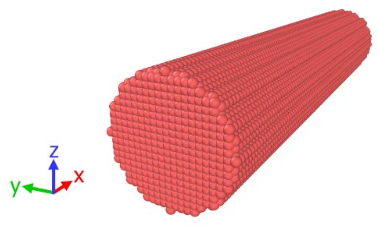
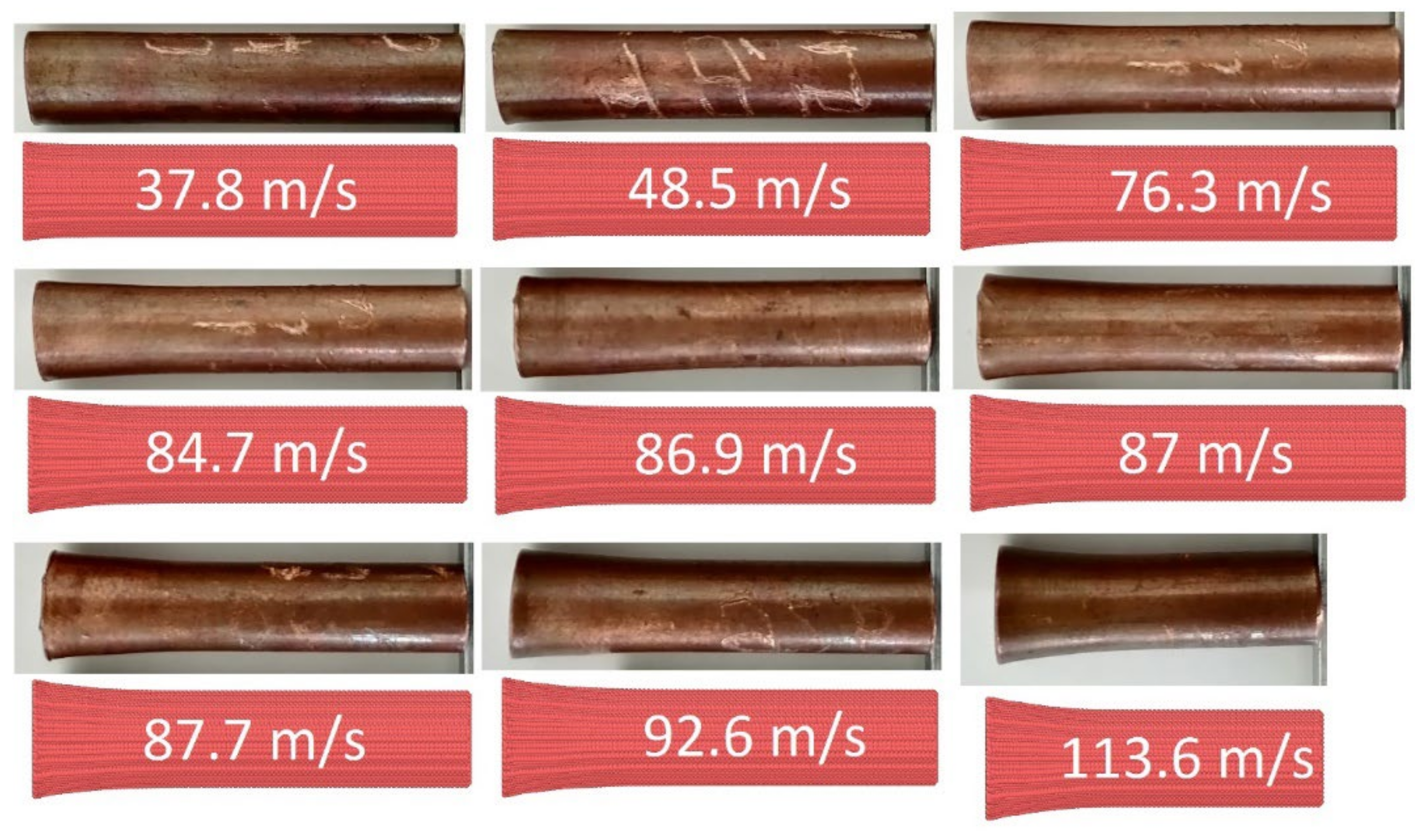

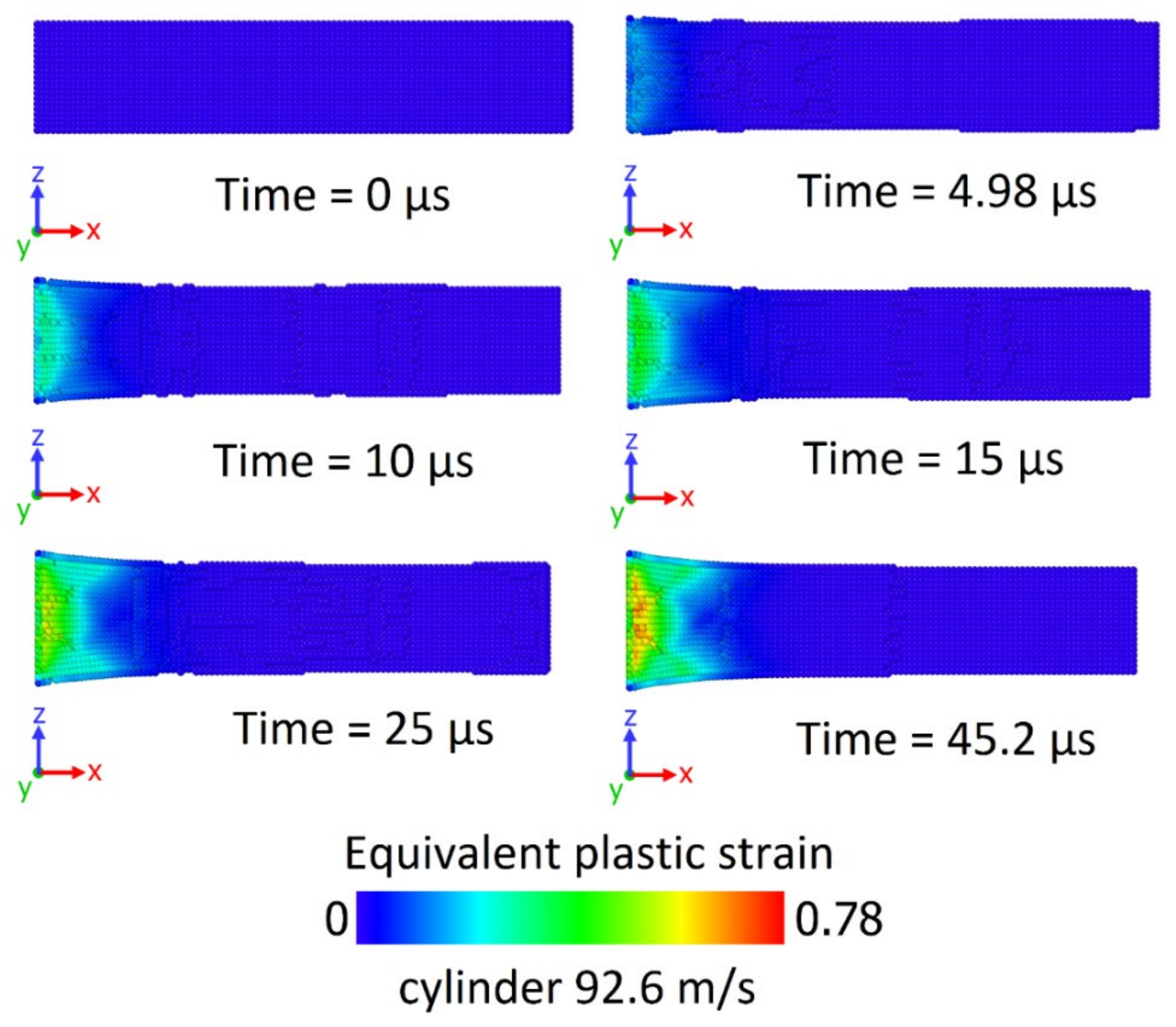
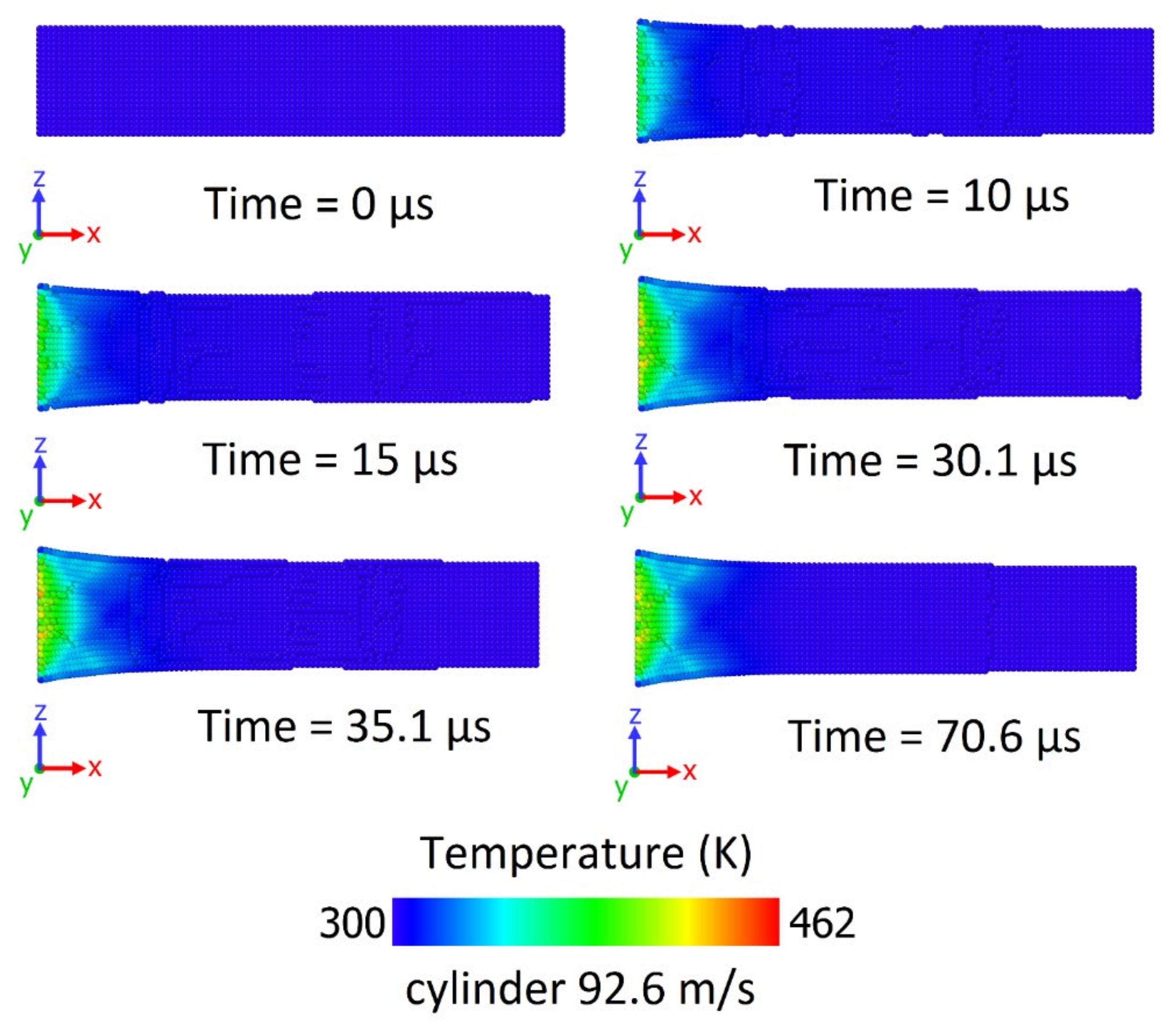
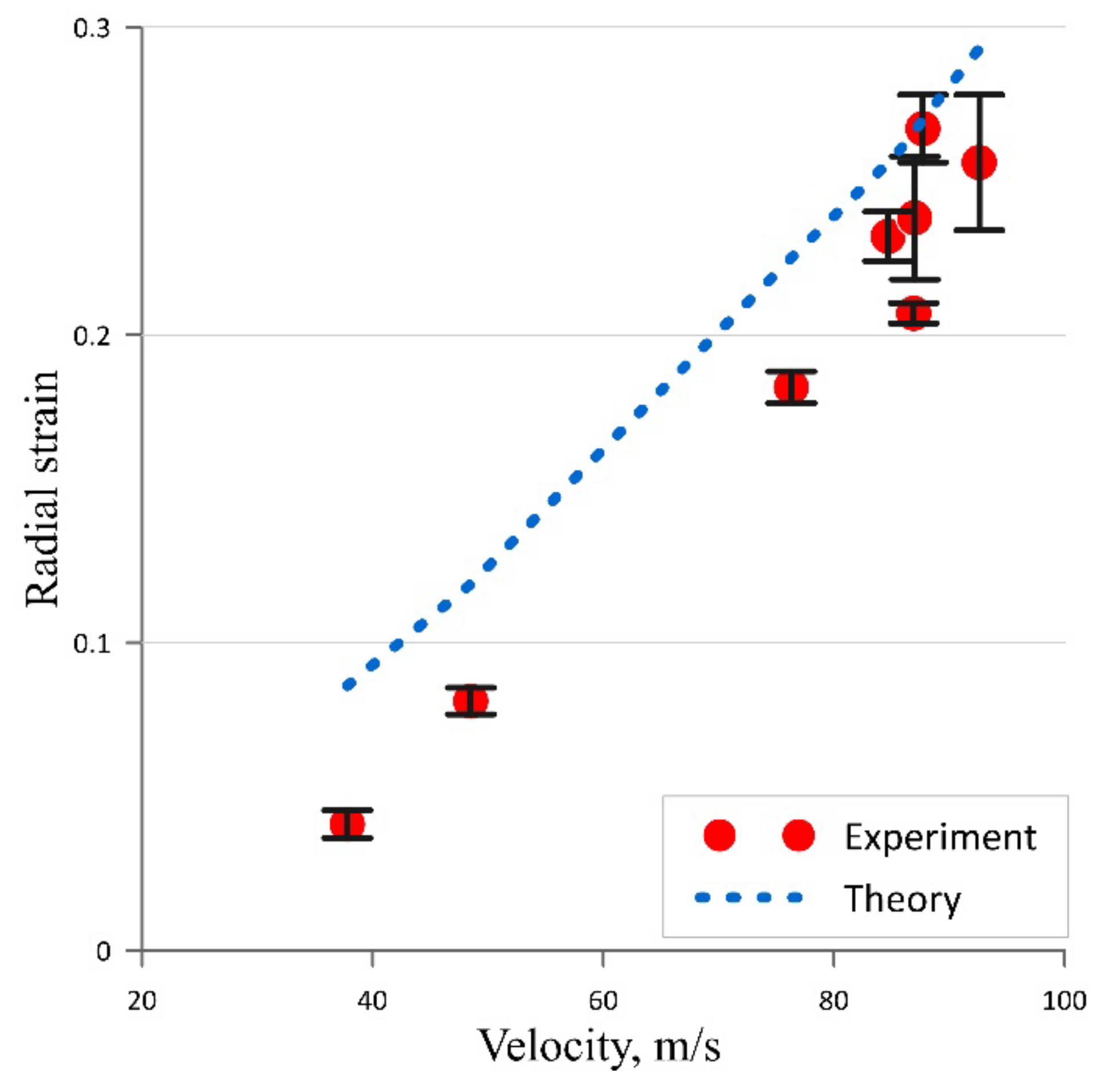

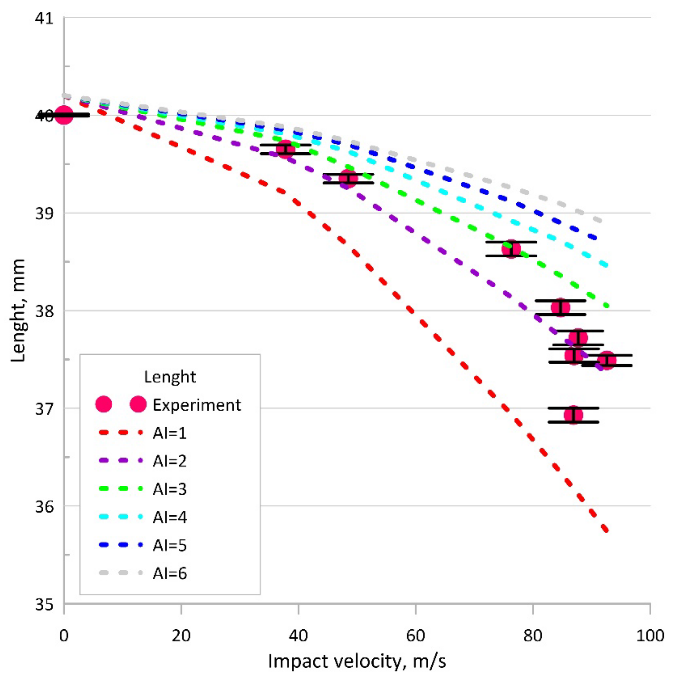
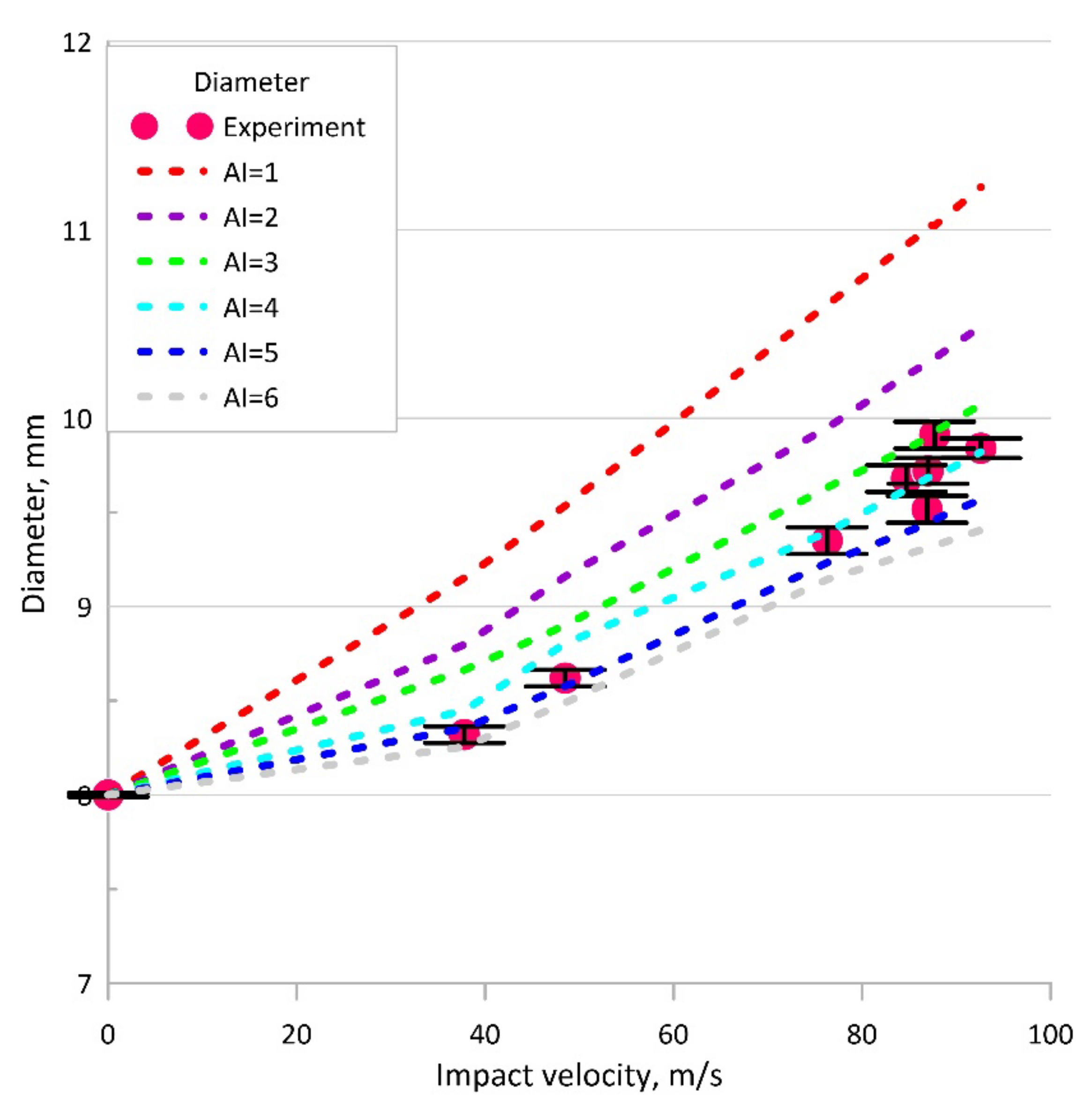
Publisher’s Note: MDPI stays neutral with regard to jurisdictional claims in published maps and institutional affiliations. |
© 2022 by the authors. Licensee MDPI, Basel, Switzerland. This article is an open access article distributed under the terms and conditions of the Creative Commons Attribution (CC BY) license (https://creativecommons.org/licenses/by/4.0/).