High-Temperature Deformation Behavior of M50 Steel

Abstract

The hot deformation characteristics of M50 steel in the temperature range of 900–1150 °C and strain-rate range of 0.01–10 s⁻¹ was investigated in this study using a Gleeble-3800 thermal simulation testing machine. The true stress–strain curves showed that the deformation resistance increased with decreasing deformation temperature, and increasing strain rate before the peak stress was reached. After the peak stress, dynamic reversion occurred, and consequently, the deformation stress decreased. The softening phenomenon was more obvious when the strain rate was low. The calculated values of the thermal deformation-activation energy Q and stress index n were 233,684.2 J/mol and 5.025568, respectively. On this basis, the Arrhenius-type constitutive equation was established, and in addition, a polynomial fit based on strain was performed to obtain the 9th-order strain-compensated constitutive equation with high fitting accuracy. By processing the flow stress curves, the processing maps of M50 steel were constructed, and the optimal processing range was predicted to be in the range of 1070–1150 °C and 0.01–1 s⁻¹. The recrystallization behavior of M50 steel was also studied by constructing a dynamic recrystallization kinetic model and combining optical microscope (OM) and electron backscatter diffraction (EBSD) observation. The results show that with the increase of deformation temperature, the degree of recrystallization transformation increased accordingly, and the original grains were gradually replaced by recrystallized grains. Besides, in the optimal process zone for thermal processing, the recrystallized grains grew with decreasing strain rate and increasing temperature.

1. Introduction

M50 steel is a kind of high-temperature bearing steel and is widely applied in the aerospace field due to its excellent mechanical properties at high temperatures [1,2,3,4,5,6]. The manufacturing process of M50 steel bearing parts usually includes forging, hot rolling, heat treatment, and machining. Hot ring rolling is the final hot deformation process that can significantly affect the final microstructure, such as carbide distribution and micro and macro defects [7,8,9]. M50 steel is a kind of high-speed steel that contains high alloying elements and large numbers of carbides [10]. Thus, the working range of M50 steel is narrow, and cracks easily form. Consequently, it is important to study the thermal deformation behavior and microstructural evolution of M50 steel.

It is well known that thermoplastic deformation is one of the significant ways to obtain excellent mechanical properties of metals. Based on the thermoplastic deformation and its results for different deformation conditions (deformation temperature, strain rate, deformation amount), a constitutive equation and thermal processing map of metals can be constructed. Dynamic Material Model (DMM)-based thermal processing maps are widely used to predict the optimal thermal processing range and guide the forging process. Peng et al. determined the constitutive equation for GCr15 steel by hot compression deformation experiments [11]. Li et al. constructed constitutive equation and processing map of 9Ni590B steel based on the flow stress curve and concluded that the optimal deformation region of 9Ni590B steel was in the temperature range of 1100–1200 °C and strain-rate range of 0.001–0.01 s⁻¹ [12]. In addition to the appropriate hot deformation parameters, the dynamic recrystallization and microstructure evolution processes are also important for the final mechanical properties. It is essential to study the entire deformation process of M50 steel and thus reveal the laws of change in the process of deformation.

In this study, the thermal deformation behavior of M50 steel under different deformation conditions was explored by thermal compression experiments under isothermal conditions using optical microscopy (OM) and electron backscatter diffraction (EBSD). On that basis, the strain-compensated intrinsic constitutive equation of M50 steel was established, and the accuracy of the model was verified, which can provide a reference for the numerical simulation of the forming process of M50 steel. The processing map of M50 steel was constructed from flow stress curves, and the optimum range of thermal processing parameters was determined. Finally, a dynamic recrystallization model of M50 steel was established, and the dynamic recrystallization mechanism was further discussed.

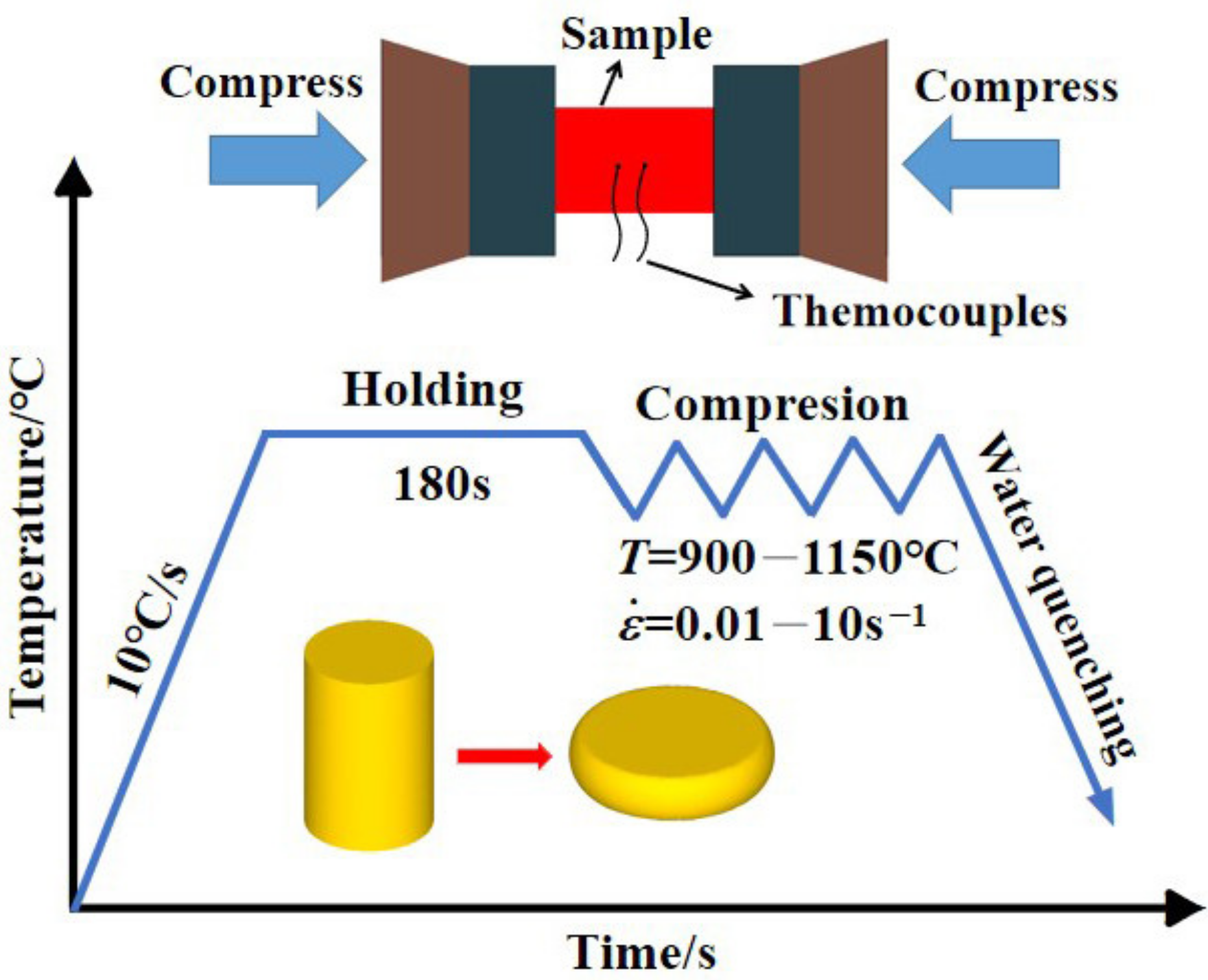
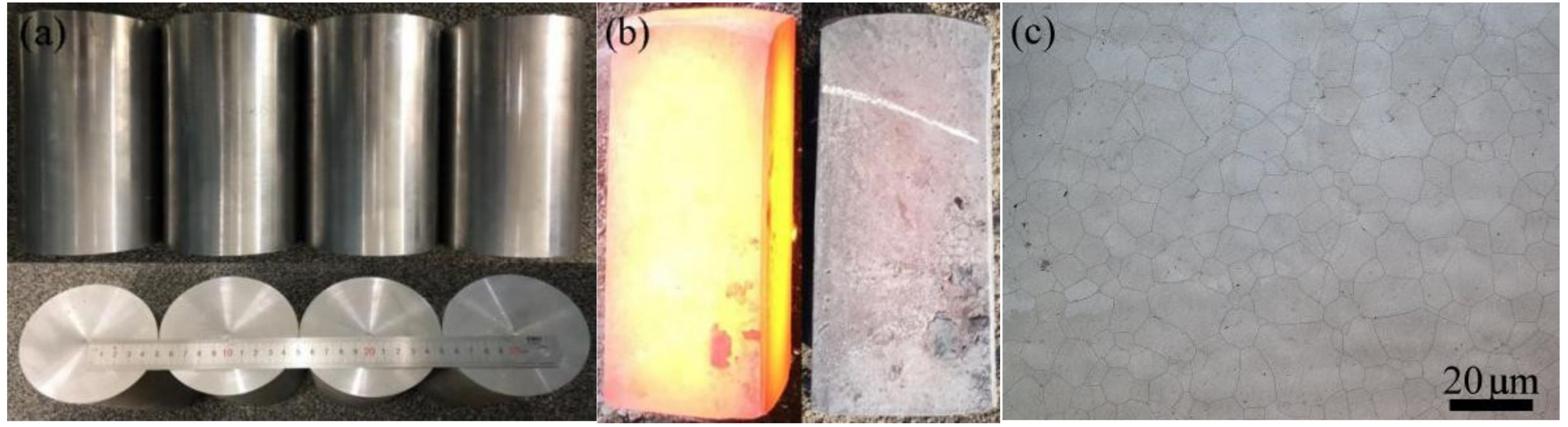
2. Experimental Procedure

The M50 steel used for the experiments was prepared by vacuum induction melting, and its chemical composition is presented in

Table 1. Chemical composition of M50 steel (mass fraction, %).

Elements	C	Cr	Mo	V	Si	Mn	Fe
Content	0.82	4.20	4.22	1.10	0.21	0.24	Bal.

. Experimental specimens with dimensions of φ 8 mm × 12 mm were cut from M50 forged specimen bars and subjected to isothermal compression experiments on a Gleeble-3800 (DSI, Troy, NY, USA) thermal simulation machine, and even at the highest strain rates tested, the test temperature was maintained ±1 °C. The experimental temperatures were 900 °C, 950 °C, 1000 °C, 1050 °C, 1100 °C, and 1150 °C and strain rates of 0.01 s⁻¹, 0.1 s⁻¹, 1 s⁻¹, and 10 s⁻¹, respectively. To deform the specimen uniformly, reduce the effect of friction on the experimental result, and avoid peculiar deformation, graphite flakes, tantalum flakes, and lubricants were pasted at both ends of the specimens. R-type thermocouple wires were soldered to the middle of the specimen for real-time temperature measurement. The specimens were heated by high-frequency induction heating, and the specimens were raised to the deformation temperature at a rate of 10 °C/s. In order to ensure the temperature uniformity during the deformation process, the specimens were held for 3 min before the hot compression test, whose total compressive strain was 70%, and the hot compression test program for M50 steel, as shown in Figure 1. Immediately after the compression test, the specimens were quenched to preserve the high-temperature microstructure, then the deformed specimens were cut along the central section parallel to the compression direction using a cut wire, mechanically ground and polished, and chemically etched for 1 min in 4% nitric acid alcohol. The microstructure was observed with an optical microscope (Zeiss, Axio Observer A1m, Jana, German) as well as a scanning electron microscope (Oxford Instruments, Abingdon, Oxfordshire, UK). The electron backscatter diffraction specimens were vibrationally polished to remove the surface deformation layer produced by mechanical grinding. Polished specimens were analyzed using a TESCAN MIRA3 field emission electron microscope with HKL Channel 5 system (Oxford Instruments, Abingdon, Oxfordshire, UK).

3. Results and Discussion

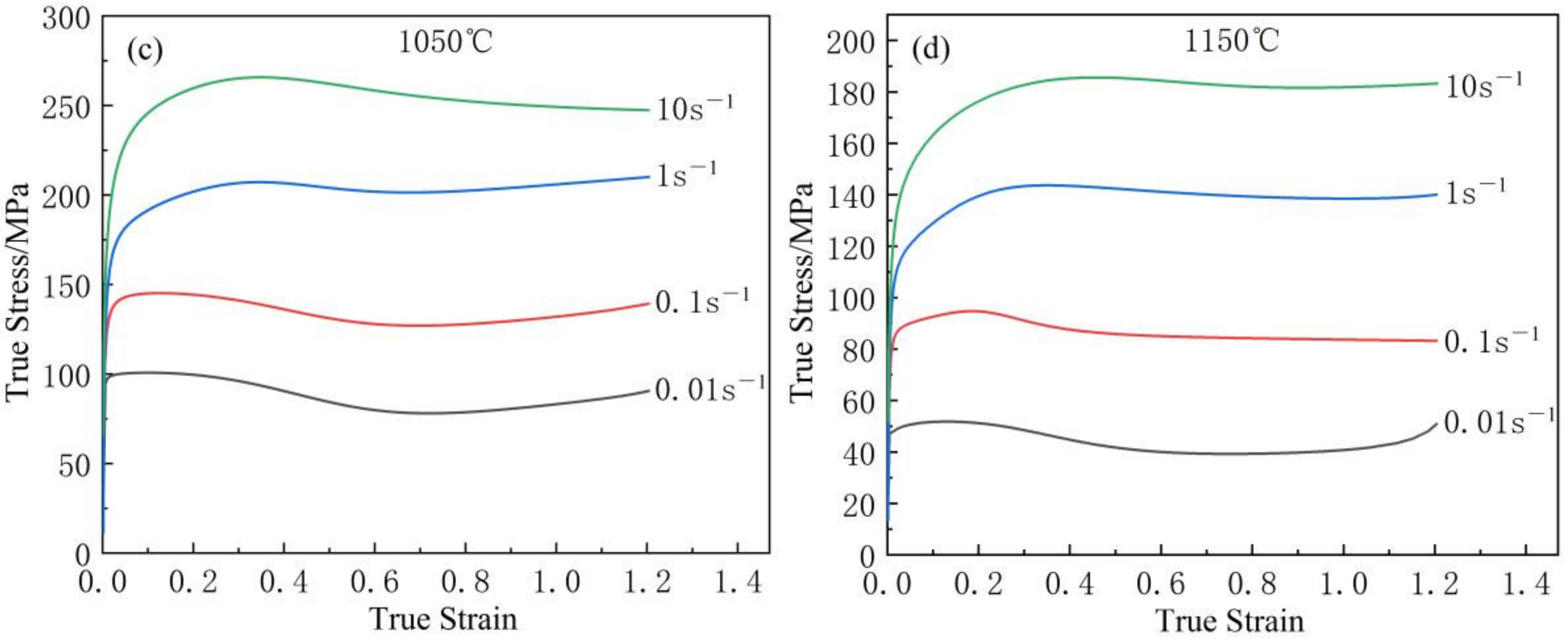
3.1. True Stress–Strain Analysis

The true stress–true strain curves of M50 steel under different deformation conditions are shown in Figure 2. It can be seen from the figure that the stress–strain curves for M50 steel all exhibit common features at different deformation temperatures. In the elastic phase, the flow stress is linearly related to the strain. During the process-hardening phase, the flow stress increases slowly due to the dislocation pile-up and the increase in dislocation density, while the softening behavior is caused by dynamic recovery (DRV), and dynamic recrystallization (DRX) is smaller. Subsequently, as the strain gradually reaches the critical strain of DRX, the stress gradually reaches its peak and gradually decreases due to the dynamic softening behavior of DRX taking the dominant position, and then, the stress-drop phase occurs. Finally, in the equilibrium stage, with increasing deformation, the process of hardening and dynamic softening reach dynamic equilibrium.

Additionally, it is also known from Figure 2d that the dynamic softening phenomenon was more obvious as the strain rate decreased after the flow stress value reached its maximum value for deformation temperature is 1150 °C. This is because the lower the strain rate and the longer the deformation process, there is sufficient time for grain boundary migration, the dislocation extinction rate is greater than the dislocation accretion rate, and the process hardening only partially offsets the dynamic softening caused by dislocation slips.

3.2. Constitutive Equation

High-temperature thermal deformation of materials is a process controlled by thermal activation, and the Arrhenius-type hyperbolic sine equation proposed by Sellars and Tegart is usually used to reveal the effects of strain rate and deformation temperature on rheological stresses [13,14]. The constitutive equation of the material can be expressed by Equation (1).

$$\dot{\epsilon }=\left\{\begin{array}{l}{A}_1{\sigma }^{n_1}\exp \left[\frac{-Q}{RT}\right],\hspace{1em}\alpha \sigma <0.8\\ A_2\exp (\beta \sigma )\exp \left[\frac{-Q}{RT}\right],\hspace{1em}\alpha \sigma >1.2\\ A{[\sinh (\alpha \sigma )]}^n\exp \left[\frac{-Q}{RT}\right],\hspace{1em}\mathrm{for} \mathrm{all}\end{array}\right.$$

(1)

where $\dot{\epsilon }$ is the strain rate, σ is the peak stress, T is the temperature, Q is the heat deformation activation energy, and R is the gas constant, which is generally taken as 8.314 J/(mol·K); A, A₁, A₂, n, n₁, α, and β are all material-dependent constants. To calculate the parameters in the equation, both sides of Equation (1) are taken logarithmically at the same time, as shown in Equations (2)–(4):

$$\ln \dot{\epsilon }=\ln A_1+n_1\ln \sigma -\frac{Q}{RT}$$

(2)

$$\ln \dot{\epsilon }=\ln A_2+\beta \sigma -\frac{Q}{RT}$$

(3)

$$\ln \dot{\epsilon }=\ln A+n\ln [\sinh (\alpha \sigma )]-\frac{Q}{RT}$$

(4)

The different deformation temperatures, strain rates and their corresponding peak stresses are substituted into Equations (2)–(4), and the $\ln \sigma \hspace{0.17em}\mathrm{with} \ln \dot{\epsilon }$, $\sigma \hspace{0.17em}\mathrm{with} \dot{\epsilon }$, and $\ln [\sinh (\alpha \sigma )]\hspace{0.17em}\mathrm{with} \ln \dot{\epsilon }$ curves can be separately obtained, as shown in Figure 3a–c. n and n₁ are the average slope of $\ln \sigma \hspace{0.17em}\mathrm{with} \ln \dot{\epsilon }$ and $\ln [\sinh (\alpha \sigma )]\hspace{0.17em}\mathrm{with} \ln \dot{\epsilon }$ and are calculated as: α = 5.026, n₁ = 6.938, and β= 0.041; hence, α = β/n₁ = 0.006.

Assuming a constant strain rate, Equation (4) is partial derivative for 1/T, and the following can be obtained:

$$Q=nR\left[\frac{\partial \ln [\sinh (\alpha \sigma )]}{\partial (1/T)}\right].$$

(5)

Substituting the deformation temperatures and peak stresses at a constant strain rate into Equation (5), $\ln [\sinh (\alpha \sigma )]\hspace{0.33em}\mathrm{with} \hspace{0.33em}1/T$ completed linear fit, as shown in Figure 3d, yields the M50 steel heat deformation activation energy Q = 233.6842 J/mol and lnA = 24.995.

Finally, by replacing the calculated values of α, n, Q, and A in Equation (1), the high-temperature thermal deformation constitutive equations of M50 steel can be obtained:

$$\dot{\epsilon }=7.165\times {10}_{}^{10}{\left[\sinh (0.006\sigma )\right]}_{}^{5.026}\exp \left(-\frac{233684.2^{}}{RT}\right).$$

(6)

Write this as a function of the Zener–Hollomon parameter:

$$\sigma =\frac{1}{0.006}\ln {\left\{{\left(\frac{Z}{7.165\times {10}^{10}}\right)}^{\frac{1}{5.026}}+{\left[\left(\frac{Z}{7.165\times {10}^{10}}\right)\right]}^{\frac{2}{5.026}}+1\right\}}^{\frac{1}{2}}.$$

(7)

3.3. Strain-Compensated Constitutive Equation

The Arrhenius model based on peak stress is not exhaustive for describing the hot deformation behavior of M50 steel under other levels of strain; Lin et al. [15]. modified the Arrhenius model based on strain. It is clear from the stress–strain curves that strain has a significant effect on the rheological stress, material parameters, and thermal deformation activation energy. It was shown that by using polynomials to express the effect of strain on the flow stress, a constitutive equation with better fitting accuracies can be obtained [16,17,18]. Therefore, this paper established a polynomial of nine times based on strain, and the fitting results are shown in Figure 4.

R² in Figure 4 shows the linear correlation coefficient of each material constant in the multiple expressions. As seen from Figure 4, the linear correlation coefficients for each material constant of the nine-fit were high, all above 0.986, indicating the high accuracy of the nine-polynomial fit. The relationship between the M50 steel material parameters (α, n, Q, and lnA) and strain can be described by Equation (8). Meanwhile, the results of the ninth-order polynomial fit are shown in

Table 2. Polynomial fitting results of α, n, Q, and lnA.

α(ε)	n(ε)	Q(ε)/(J·mol−1)	lnA(ε)
a0 = 0.006	n0 = 7.507	Q0 = 2.436 × 105	A0 = 27.294
a1 = 0.033	n1 = −50.447	Q1 = 2.338 × 105	A1 = −26.304
a2 = −0.496	n2 = 490.730	Q2 = −3.254 × 106	A2 = 276.562
a3 = 3.022	n3 = −2602.976	Q3 = 1.701 × 107	A3 = −1768.519
a4 = −9.916	n4 = 7986.397	Q4 = −5.1519 × 107	A4 = 6060.06
a5 = 19.426	n5 = −14,973.221	Q5 = 9.562 × 107	A5 = −12,314.872
a6 = −23.375	n6 = 17,437.466	Q6 = −1.097 × 108	A6 = 15,343.242
a7 = 16.926	n7 = −12,306.306	Q7 = 7.581 × 107	A7 = −11,495.234
a8 = −6.765	n8 = 4817.502	Q8 = −2.891 × 107	A8 = 4750.641
a9 = 1.146	n9 = −802.37	Q9 = 4.673 × 106	A9 = −831.691

.

$$\left\{\begin{array}{l}\alpha ={\alpha }_0+{\alpha }_1\epsilon +{\alpha }_2{\epsilon }^2+{\alpha }_3{\epsilon }^3+\cdots +{\alpha }_8{\epsilon }^8+{\alpha }_9{\epsilon }^9\\ n=n_0+n_1\epsilon +n_2{\epsilon }^2+n_3{\epsilon }^3+\cdots +n_8{\epsilon }^8+n_9{\epsilon }^9\\ Q=Q_0+Q_1\epsilon +Q_2{\epsilon }^2+Q_3{\epsilon }^3+\cdots +Q_8{\epsilon }^8+Q_9{\epsilon }^9\\ \ln A=A_0+A_1\epsilon +A_2{\epsilon }^2+A_3{\epsilon }^3+\cdots +A_8{\epsilon }^8+A_9{\epsilon }^9\end{array}\right.$$

(8)

According to the hyperbolic rule, by substituting Equation (8) into Equation (1) and combining the ninth-order polynomial coefficients from Table 2, the stress equation for M50 steel based on strain compensation is expressed as a Z function.

$$\left\{\begin{array}{l}Z=\dot{\epsilon }\exp (\frac{Q}{RT})\\ \sigma =\frac{1}{\alpha (\epsilon )}\ln \left\{{(\frac{Z}{A(\epsilon )})}^{\frac{1}{n(\epsilon )}}+\left[{(\frac{Z}{A(\epsilon )})}^{\frac{2}{n(\epsilon )}}+1\right]\left.\begin{array}{l}{}^{\frac{1}{2}}\\ \end{array}\right\}\right.\end{array}\right.$$

(9)

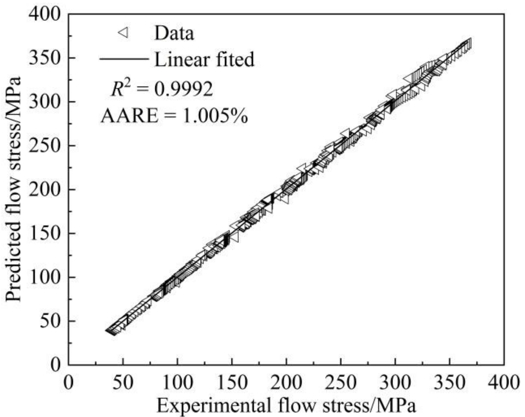
3.4. Verification of the Strain-Compensated Constitutive Equation

The constructed strain-compensated constitutive equation is used to predict the corresponding flow stress values under different deformation conditions, and the comparison between the predicted and experimental values of flow stress is shown in Figure 5, which shows that the predicted values of flow stresses from the strain-compensated constitutive equation are in good agreement with the experimental values.

The degree of linear correlation between the predicted value of flow stress and the experimental value can be evaluated by the correlation coefficient R². A graph of the relationship between the predicted value of flow stress and the experimental value is constructed, as shown in Figure 6, from which it can be seen that the correlation coefficient R² is 0.9992, indicating a high degree of correlation between the predicted value of flow stress and the experimental value. In this paper, the average absolute error (AARE) was also used to calculate the overall absolute error value between the predicted and experimental values of the flow stress, as shown in Figure 6, and an average relative error of 1.005% was calculated for all data.

In summary, the predicted flow stresses based on the strain-compensated constitutive equation have good agreement with the experimental values under different deformation conditions, the linear correlation coefficient R² between the predicted and experimental values reaches 0.998, and the average absolute error value between all the predicted and experimental flow stresses is only 1.005%, which indicates that the strain-compensated constitutive equation can accurately predict the flow stresses in the present experimental range.

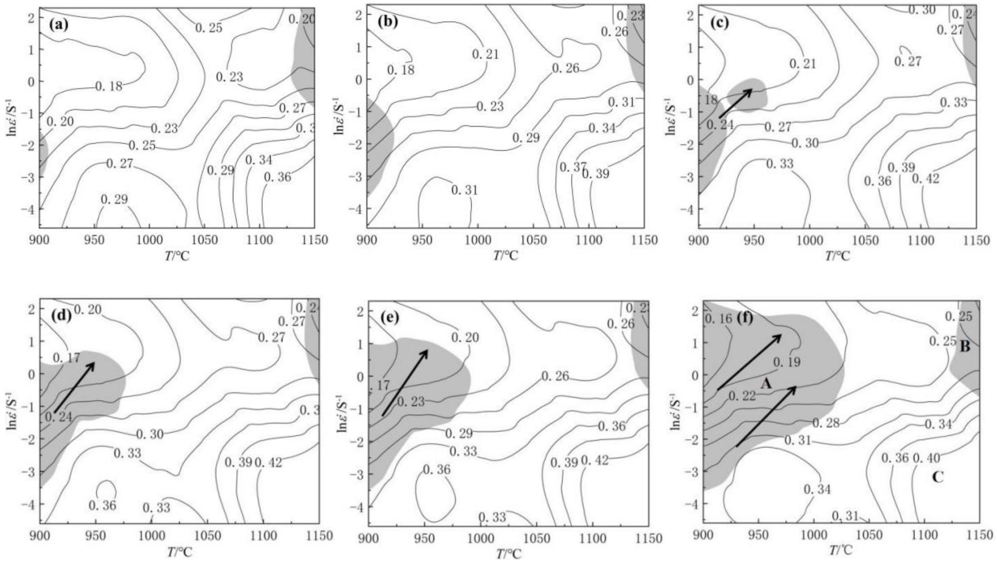
3.5. Processing Maps

The processing map was proposed by Prasad [19] based on the dynamic material model (DMM) theory, which aims to study the processability of materials during thermal deformation. The total energy P input during thermal deformation can be divided into the dissipated energy G consumed by plastic deformation and the dissipated energy J consumed by microstructure evolution during deformation in the DMM theory. Both components can be represented by strain rate and flow stress, which is expressed as [20]:

$$P=\sigma \dot{\epsilon }=G+J={\displaystyle {\int }_0^{\dot{\epsilon }}\sigma }d\dot{\epsilon }+{\displaystyle {\int }_0^{\sigma }\dot{\epsilon }d\sigma }$$

(10)

where P is the total dissipation energy of plastic deformation, G is the plastic deformation dissipation value, and J is the dissipation value due to microstructural changes. To ensure the accuracy of the resultant data, the relationship between flow stress and strain rate was fitted with a third-order polynomial [21].

$$\lg \sigma =a+b\lg \dot{\epsilon }+b_1{(\lg \dot{\epsilon })}^2+b_2{(\lg \dot{\epsilon })}^3$$

(11)

The corresponding third-order fits lead to a, b, b₁, and b₂. Derivation of Equation (11) yields the expression for the strain-rate-sensitive parameter m:

$$m=b+2b_1\lg \dot{\epsilon }+3b_2{(\lg \dot{\epsilon })}^2.$$

(12)

When the strain rate sensitivity index m = 1, the maximum value of dissipation J due to microstructural changes is $\sigma \dot{\epsilon }/2$. The power dissipation rate can be expressed η:

$$\eta =\frac{J}{J_{\max }}=\frac{\sigma \dot{\epsilon }-{\displaystyle {\int }_0^{\dot{\epsilon }}\sigma d\dot{\epsilon }}}{(\sigma \dot{\epsilon }/2)}=\frac{2m}{m+1}.$$

(13)

The power dissipation diagram is composed of η versus deformation rate and deformation temperature, and the contour plot of η indicates the energy dissipation value of the material, which describes the energy dissipation due to changes in the microstructure of the material [22]. Establishing a cubic polynomial of η versus $\ln \dot{\epsilon }$ [23].

$$\ln \left(\frac{m}{m+1}\right)=b+b_1\ln \dot{\epsilon }+b_2{\left(\ln \dot{\epsilon }\right)}^2+b_3{\left(\ln \dot{\epsilon }\right)}^3.$$

(14)

To further discuss the effect of the deformation rate on the plastic forming of the material, Ziegler [24] proposed characterizing the instability region of plastic deformation in terms of the instability parameter ξ. The expression is given in Equation (15).

$$\xi (\dot{\epsilon })=\frac{\partial \ln (m/(m+1))}{\partial \ln \dot{\epsilon }}+m<0.$$

(15)

The processing maps of the specimens under different strains are shown in Figure 7, where the white area is the safety zone, and the gray area (ξ < 0) is the destabilization region. As shown in the figures, when the true strain is 0.2, there is a destabilization zone in the low- and high-strain-rate regions, which are 900–910 °C, 0.04–0.2 s⁻¹, and 1125–1150 °C, 0.5–10 s⁻¹, respectively, and the maximum power dissipation value is 0.36. As the true strain increases to 0.6, the two instability regions expand with a maximum power dissipation value of 0.42. The instability region was extended from the low-strain-rate region to the high-strain-rate region, and the instability regions were from 900 to 1025 °C, 0.04 to 10 s⁻¹ and 1120 to 1050 °C, 0.2 to 10 s⁻¹, with a maximum power dissipation value of 0.4 when the true strain increased to 1.2. This results in a zone of instability for M50 steel at 70% deformation; however, the best forging area is away from the area of instability and in the region of higher power dissipation values. According to the true strain of the 1.2 processing map, the optimal processing range for M50 steel is obtained as follows: 1070 to 1150 °C, 0.01 to 1 s⁻¹.

Figure 8 shows the locations of the three regions A, B, and C on the hot working map with a strain of 1.2, corresponding to the observation of the microstructure in the destabilization region and the safety region. The destabilized A region has many fine recrystallized grains distributed at its grain boundaries at low temperature and high strain rate, and dynamic recrystallization does not occur completely, as shown in Figure 8a. Figure 8b shows a large number of fine, dynamically recrystallized grains distributed in the microstructure at high temperature and high strain rate due to its short deformation time, which makes the dynamic recrystallization process not finished, and a small amount of original grains exist. Dynamic recrystallization occurs completely, and the microstructures are all fine and uniform at high temperature and low strain rate (1150 °C, 0.1 s⁻¹), as shown in Figure 8c.

The process conditions of a deformation temperature of 1150 °C and strain rate of 1 s⁻¹ were selected in the optimal hot working range (1070 to 1150 °C, 0.01 to 1 s⁻¹) of M50 steel and forged for M50 steel of size φ100 × 180, as shown in Figure 9a. It was forged by 750 Kg hydraulic press and annealed treatment by heat treatment furnace. The M50 steel specimens had good surface quality during forging and after annealing treatment, with no cracks or pits, as shown in Figure 9b. A 10 mm × 10 mm × 8 mm specimen was obtained in the center of the cross-section of the annealed M50 steel intermediate section, and the specimen grains were observed using an optical microscope. Figure 9c shows that the grains are equiaxed recrystallized grains with a uniform grain distribution. This shows that the process conditions of a deformation temperature of 1150 °C and strain rate of 1 s⁻¹ can be used as the forging process for M50, and in addition, it also proves that the optimal processing range obtained from the hot working diagram of M50 steel is reliable. The optimal forging process for M50 steel can provide technical guidance for actual forging production.

3.6. Modeling of Dynamic Recrystallization

Dynamic recrystallization occurs when the strain reaches the critical strain value; therefore, the critical strain is an important parameter for the dynamic recrystallization of the material. In this paper, the method proposed by Poliak [25] is used to draw the θ-σ curves based on the work-hardening rate θ (θ = dσ/dε) of the true stress curve, as shown in Figure 10a. The two intersection points of the curve with θ = 0 are peak stress σ_p and steady-state stress σ_ss. The inflection point (σc) on the θ-σ curve is the critical stress, whose exact location is difficult to determine; therefore, the ψ(−dθ/dσ)-σ curve is obtained by taking the derivative of the θ-σ curve as shown in Figure 10b, and the maximum value point is the critical stress σ_c. The critical stress point is determined in Figure 10a and a tangent line to intersect θ = 0 for the saturation stress σ_s.

The evolution of dynamic recrystallization usually consists of three stages: the initial latent phase, the accumulation phase, and the steady-state phase [26]. The dynamic expression for dynamic recrystallization is Equation (16) when the strain rate is constant [27].

$$X_{DRX}=1-\exp \left(-k_{DRX}{\left(\frac{\epsilon -{\epsilon }_c}{{\epsilon }_p}\right)}^{n_{DRX}}\right)$$

(16)

where X_DRX represents the volume fraction of dynamic recrystallization, and k_DRX and n_DRX are material constants. The expression for the flow stress versus the volume fraction of dynamic recrystallization is given in Equation (17) [28].

$$X_{DRX}=\frac{{\sigma }_{\mathrm{P}}-\sigma }{{\sigma }_P-{\sigma }_{SS}}$$

(17)

where σ_p is the peak stress, and σ_ss is the steady-state stress.

The dynamic recrystallization volume fraction of Equation (17) is substituted into Equation (16) and taken logarithmically to obtain Equation (18).

$$\ln [-\ln (1-X_{DRX})]=\ln k_{DRX}+n_{DRX}\ln [(\epsilon -{\epsilon }_C)/{\epsilon }_P].$$

(18)

Figure 11 shows the relationship curve of ln[−ln(1 − X_DRX)] − ln[(ε − ε_c)/ε_p] with the slope of material constant n_DRX and the intercept of ln k_DRX. The average value of material constant n_DRX under different deformation conditions is 5.024, and the average value of material constant k_DRX is 0.334 by linear fitting.

$$X_{DRX}=1-\exp \left[-0.334{(\frac{\epsilon -{\epsilon }_C}{{\epsilon }_P})}^{5.204}\right].$$

(19)

3.7. Microstructure Evolution

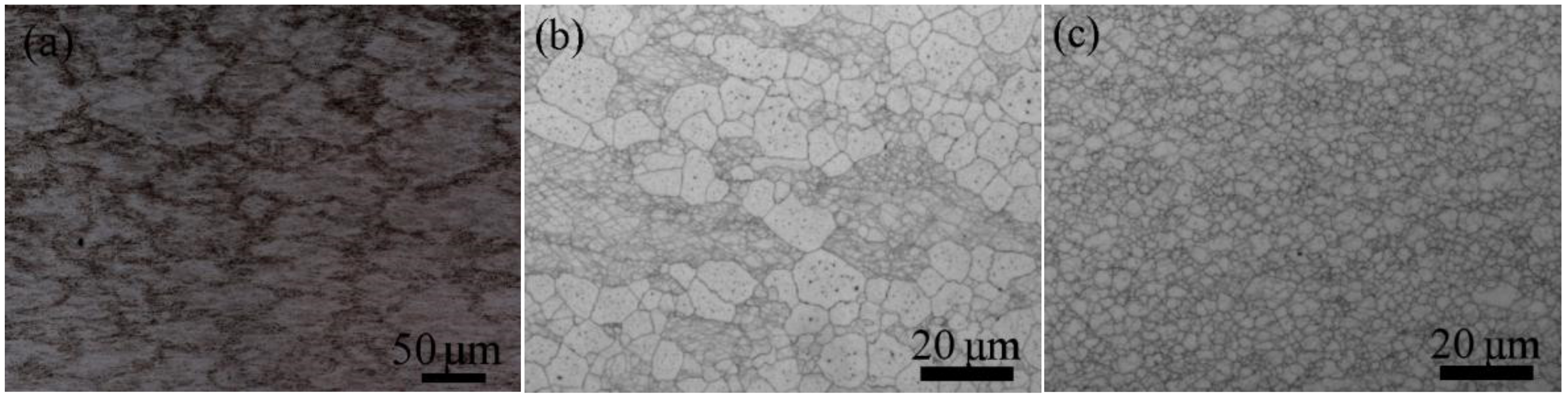
3.7.1. Microstructure of Thermal Deformation

The finite element software DEFORM was used to conduct high-temperature, single-pass hot compression simulation experiments of M50 steel. By intercepting the specimen along the diameter direction after simulated compression, the deformation results at different locations on the longitudinal section can be obtained, as shown in Figure 12, which shows the equivalent effect variation cloud diagram and its corresponding microstructure at 1100 °C, 0.1 s⁻¹, and 70% hot compression conditions. In the process of thermal deformation, due to the difference in force and metal flow at various locations resulting in different degrees of deformation across regions, the equivalent effect of the value of deformation can be seen as region (c) > region (b) > region (a). The direction of metal flow in the process of thermal deformation is shown by the black arrow in the figure. From Figure 12, it can be seen that the microstructure of each region is closely related to the degree of deformation of the corresponding position of the specimen after compression, and the whole longitudinal section of the compressed specimen is divided into three deformation zones. Due to the low temperature and high friction, the metal flow is difficult, the deformation is small, the deformation storage energy is low, and it is difficult to reach the critical point of recrystallization energy requirement, making region (a) a difficult deformation zone, and only at the grain boundaries to reach the recrystallization critical point, as seen from Figure 12a, only a small portion of fine recrystallized grains appear near some of the grain boundaries. Region (c) is a large deformation zone, and larger deformation can result in high-deformation energy storage; this region of the material can achieve complete dynamic recrystallization; therefore, region (c) has a uniform distribution of fine recrystallization organization, as shown in Figure 12c. Region (b) is a small deformation zone, and the large deformation in the region (c) makes the metal flow outward, applying compressive stresses to the region (b), which causes tensile stresses in the tangential direction, causing the dynamically recrystallized grains in this region to vary in size. Figure 12b shows that this region has been almost completely transformed into dynamically recrystallized grains, but the recrystallized grains have large differences in size.

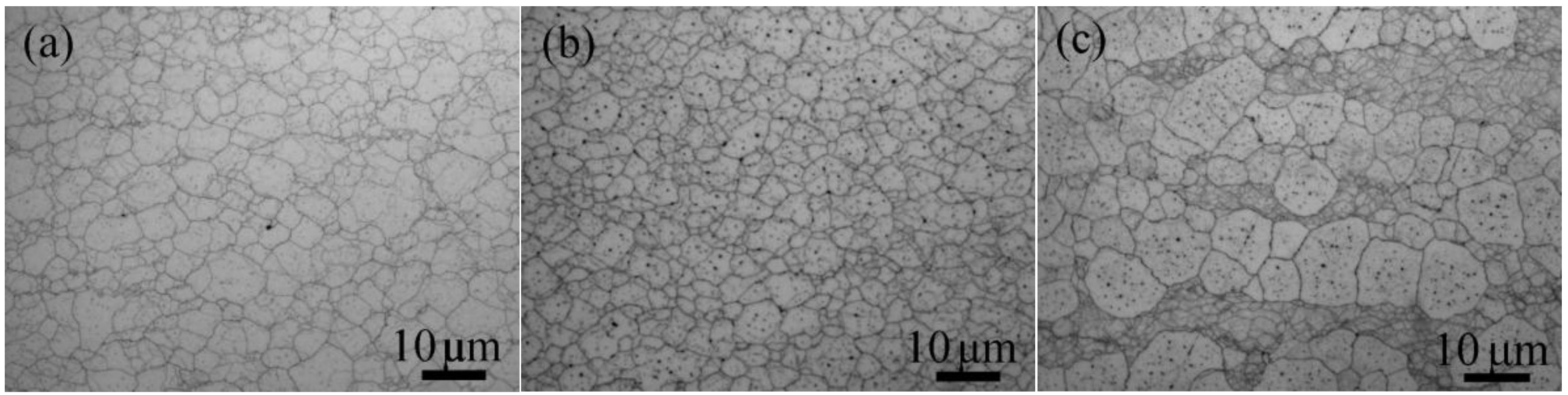
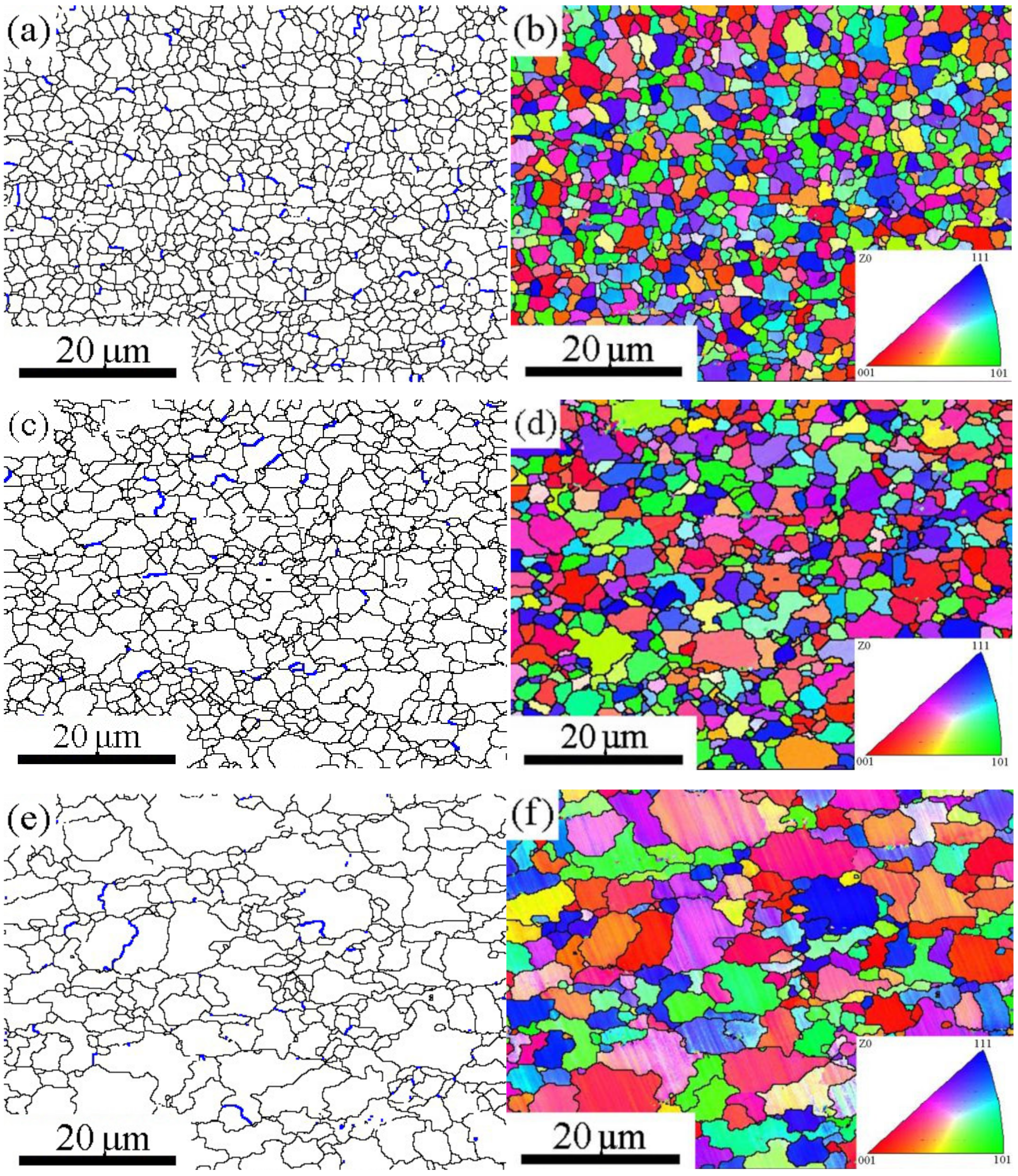
3.7.2. Microstructural Evolution of Dynamic Recrystallization

Through the above study of thermal deformation at different locations of the specimen cross-section after compression of M50, the microstructure observation of the large deformation zone of the specimen cross-section after compression under deformation conditions was continued. The microstructure of M50 steel at different deformation temperatures at a strain rate of 0.1 s⁻¹ is given in Figure 13. Figure 13a shows that the grains elongated along the deformation direction at a temperature of 950 °C. Furthermore, there are fine recrystallized grains at the grain boundaries due to the occurrence of dynamic recrystallization. The reason for this phenomenon is that during the thermal deformation of M50 steel, the generated and extinguished dislocations on both sides of the grain boundary trigger unequal distortion storage energy on both sides of the grain boundary, causing the grain boundary to migrate to the side with high-distortion storage energy, which in turn leads to the formation of a small number of fine dynamic recrystallized grains along the original grain boundary [29]. The original grains were replaced by fine dynamic recrystallized grains, leaving only a few “long” original grains when the temperature rose to 1050 °C, as shown in Figure 13b. When the deformation temperature was further increased to 1150 °C, the recrystallization process tended to be completed, and the original grains were completely replaced by equiaxed grains of smaller size, as shown in Figure 13c.

Figure 14 shows the metallographic organization of M50 steel at 1150 °C for different strain rates. It can be seen that at the low strain rate of 1150 °C, the grains have been completely recrystallized due to the high temperature and sufficient time for the deformation process, as shown in Figure 14a,b. However, at a strain rate of 10 s⁻¹, only a small number of fine recrystallized grains exist. The reason is that although the strain is much higher than the critical strain, the deformation process was very rapid at the high strain rate, making the inhomogeneous of microstructure, and a large number of original grains were not transformed into recrystallized grains at 1150 °C and 70% deformation, as shown in Figure 14c.

Figure 15 shows the microstructure for different deformation conditions obtained by EBSD characterization of the optimal machining range in the working maps of M50 steel. As shown in Figure 15a,c,e, the original microstructure almost completely generated a dynamic recrystallization organization with large angular grain boundaries in the hot working range of M50 steel. Figure 15b,d shows the finer microstructure for higher strain rates at the same deformation temperature and different strain rates. This can be attributed to the fact that when deformation is intense at high strain rates, the microstructure may undergo deformation to allow dislocations to form within it, reducing the strain gradient between the deformed microstructure and therefore making the growth of the microstructure insignificant. At low strain rates, the microstructure grows significantly as the temperature increases, as shown in Figure 15d,f. This is because the deformation temperature provides the impetus for the growth of the microstructure when the original microstructure tends to be fully transformed, and the growth becomes more pronounced with the increase in deformation temperature [30].

4. Conclusions

In this paper, isothermal compression tests were conducted on M50 steel on a Gleeble 3800 thermal simulation tester at temperatures of 900–1150 °C and strain rates of 0.01–10 s⁻¹. The main conclusions from the study of the thermal deformation behavior of M50 steel are as follows:

• By analyzing the flow stress curves, it is known that the deformation resistance of M50 steel increases with decreasing deformation temperature and increasing strain rate before the peak stress is reached, and after the peak stress, there is an obvious dynamic recovery. The heat deformation-activation energy Q = 233,684.2 J/mol for M50 steel is obtained after processing the flow stress curves, and the heat deformation constitutive equation established is:

$$\sigma =\frac{1}{0.006}\ln {\left\{{\left(\frac{Z}{7.165\times {10}^{10}}\right)}^{\frac{1}{5.026}}+{\left[\left(\frac{Z}{7.165\times {10}^{10}}\right)\right]}^{\frac{2}{5.026}}+1\right\}}^{\frac{1}{2}}.$$

2.

A polynomial fit of order 9 was used to establish the strain-compensated constitutive equation, which was verified and the linear correlation coefficient R2 was found to be 0.998 with an average absolute error value of 1.005%, indicating that the strain-compensated constitutive equation is highly reliable and can accurately predict the flow stress values within the present experimental range.

3.

Based on the thermal processing maps, the optimum processing range for the hot working process of M50 steel was determined: deformation temperature 1070–1150 °C and strain rate 0.01–1 s⁻¹. By fitting and analyzing the flow stress curve of M50 steel, the expression of the dynamic recrystallization iso-mechanical model of M50 steel during thermal deformation is constructed as follows:

$$X_{DRX}=1-\exp \left[-0.334{(\frac{\epsilon -{\epsilon }_C}{{\epsilon }_P})}^{5.204}\right].$$

4.

During the thermal deformation process, the higher deformation energy storage enables the large deformation zone to obtain more completely recrystallized grains. At low temperatures and low strain rates, a small number of fine recrystallized grains exist at the original grain boundaries, which are gradually replaced by recrystallized grains as the temperature increases. In the best processing range of hot working, the original grains were completely transformed into recrystallized grains, and the microstructure grew with decreasing strain rate and increasing temperature.

References

1. Rosado, L.; Trivedi, H.K.; Gerardi, D.T. Evaluation of fatigue and wear characteristics of M50 steel using high temperature synthetic turbine engine lubricants—Part II. Wear 1996, 196, 133–140. [Google Scholar] [CrossRef]
2. Elsheikh, A.H.; Yu, J.; Sathyamurthy, R.; Tawfik, M.; Shanmugan, S.; Essa, F. Improving the tribological properties of AISI M50 steel using Sns/Zno solid lubricants. J. Alloy. Compd. 2020, 821, 153494. [Google Scholar] [CrossRef]
3. Braza, J.; Pearson, P. Tribological and Metallurgical Evaluation of Ferritic Nitrocarburized M-50 and M-50 NiL Steels. ASTM Spec. Tech. Publ. 2009, 1, 49–60. [Google Scholar] [CrossRef]
4. Braza, J.F.; Pearson, P.K.; Hannigan, C.J. The Performance of 52100, M-50, and M-50 NiL Steels in Radial Bearings. SAE Tech. Pap. 1993, 102, 437–449. [Google Scholar] [CrossRef]
5. Bhadeshia, H. Steels for bearings. Prog. Mater. Sci. 2012, 57, 268–435. [Google Scholar] [CrossRef]
6. Orlov, M.R.; Grigorenko, V.B.; Morozova, L.V.; Naprienko, S.A. Research of operational damages of bearings by methods of optical microscopy, scanning electron microscopy and X-ray microanalysis. Proc. VIAM 2016, 1, 62–79. [Google Scholar] [CrossRef]
7. Jiang, H.W.; Song, Y.R.; Wu, Y.C.; Shan, D.B.; Zong, Y.Y. Macrostructure, microstructure and mechanical properties evolution during 8Cr4Mo4V steel roller bearing inner ring forging process. Mat. Sci. Eng. A 2020, 798, 140196. [Google Scholar] [CrossRef]
8. Jiang, H.; Shan, D.; Guo, B.; Zong, Y. Effect of fibrous macrostructure on mechanical properties, anisotropy and fracture mechanism of roller bearing ring. Mater. Sci. Eng. A 2021, 816, 141311. [Google Scholar] [CrossRef]
9. Zhang, C.; Peng, B.; Wang, L.; Ma, X.; Gu, L. Thermal-induced surface damage of M50 steel at rolling-sliding contacts. Wear 2019, 420, 116–122. [Google Scholar] [CrossRef]
10. Mukhopadhyay, P.; Kannaki, P.; Srinivas, M.; Roy, M. Microstructural developments during abrasion of M50 bearing steel. Wear 2014, 315, 31–37. [Google Scholar] [CrossRef]
11. Peng, N.-Q.; Tang, G.-B.; Yao, J.; Liu, Z.-D. Hot Deformation Behavior of GCr15 Steel. J. Iron Steel Res. Int. 2013, 20, 50–56. [Google Scholar] [CrossRef]
12. Li, R.; Chen, Y.; Jiang, C.; Zhang, R.; Fu, Y.; Huang, T.; Chen, T. Hot Deformation Behavior and Processing Maps of a 9Ni590B Steel. J. Mater. Eng. Perform. 2020, 29, 3858–3867. [Google Scholar] [CrossRef]
13. Sellars, C.; McTegart, W. On the mechanism of hot deformation. Acta Met. 1966, 14, 1136–1138. [Google Scholar] [CrossRef]
14. Haghdadi, N.; Zarei-Hanzaki, A.; Abedi, H.R. The flow behavior modeling of cast A356 aluminum alloy at elevated temperatures considering the effect of strain. Mater. Sci. Eng. A 2011, 535, 252–257. [Google Scholar] [CrossRef]
15. Lin, Y.; Chen, M.-S.; Zhong, J. Constitutive modeling for elevated temperature flow behavior of 42CrMo steel. Comput. Mater. Sci. 2008, 42, 470–477. [Google Scholar] [CrossRef]
16. Ou, L.; Nie, Y.; Zheng, Z. Strain Compensation of the Constitutive Equation for High Temperature Flow Stress of a Al-Cu-Li Alloy. J. Mater. Eng. Perform. 2013, 23, 25–30. [Google Scholar] [CrossRef]
17. Nayak, K.C.; Date, P.P. Development of Constitutive Relationship for Thermomechanical Processing of Al-SiC Composite Eliminating Deformation Heating. J. Mater. Eng. Perform. 2019, 28, 5323–5343. [Google Scholar] [CrossRef]
18. Dong, Y.; Zhang, C.; Lu, X.; Wang, C.; Zhao, G. Constitutive Equations and Flow Behavior of an As-Extruded AZ31 Magnesium Alloy Under Large Strain Condition. J. Mater. Eng. Perform. 2016, 25, 2267–2281. [Google Scholar] [CrossRef]
19. Prasad, Y.V.R.K.; Gegel, H.L.; Doraivelu, S.M.; Malas, J.C.; Morgan, J.T.; Lark, K.A.; Barker, D.R. Modeling of dynamic material behavior in hot deformation: Forging of Ti-6242. Metall. Trans. A 1984, 15, 1883–1892. [Google Scholar] [CrossRef]
20. Prasad, Y.; Rao, K. Processing maps and rate controlling mechanisms of hot deformation of electrolytic tough pitch copper in the temperature range 300–950 °C. Mater. Sci. Eng. A 2005, 391, 141–150. [Google Scholar] [CrossRef]
21. Tan, Y.; Yang, L.; Tian, C.; Liu, W.; Liu, R.; Zhang, X. Processing maps for hot working of 47Zr–45Ti–5Al–3V alloy. Mater. Sci. Eng. A 2014, 597, 171–177. [Google Scholar] [CrossRef]
22. Zhang, J.; Di, H.; Mao, K.; Wang, X.; Han, Z.; Ma, T. Processing maps for hot deformation of a high-Mn TWIP steel: A comparative study of various criteria based on dynamic materials model. Mater. Sci. Eng. A 2013, 587, 110–122. [Google Scholar] [CrossRef]
23. Mirzadeh, H.; Najafizadeh, A. Hot Deformation and Dynamic Recrystallization of 17-4 PH Stainless Steel. ISIJ Int. 2013, 53, 680–689. [Google Scholar] [CrossRef] [Green Version]
24. Ziegler, H.; Carlson, D.E. An Introduction to Thermomechanics. J. Appl. Mech. 1978, 45, 966. [Google Scholar] [CrossRef] [Green Version]
25. Poliak, E.; Jonas, J. A one-parameter approach to determining the critical conditions for the initiation of dynamic recrystallization. Acta Mater. 1996, 44, 127–136. [Google Scholar] [CrossRef]
26. Chen, X.; Du, Y.; Du, K.; Lian, T.; Liu, B.; Li, Z.; Zhou, X. Identification of the Constitutive Model Parameters by Inverse Optimization Method and Characterization of Hot Deformation Behavior for Ultra-Supercritical Rotor Steel. Materials 2021, 14, 1958. [Google Scholar] [CrossRef]
27. Kong, L.; Hodgson, P.; Wang, B. Development of constitutive models for metal forming with cyclic strain softening. J. Mater. Process. Technol. 1999, 89, 44–50. [Google Scholar] [CrossRef]
28. Zhang, P.; Yi, C.; Chen, G.; Qin, H.; Wang, C. Constitutive Model Based on Dynamic Recrystallization Behavior during Thermal Deformation of a Nickel-Based Superalloy. Metals 2016, 6, 161. [Google Scholar] [CrossRef] [Green Version]
29. Sakai, T.; Belyakov, A.; Kaibyshev, R.; Miura, H.; Jonas, J.J. Dynamic and post-dynamic recrystallization under hot, cold and severe plastic deformation conditions. Prog. Mater. Sci. 2014, 60, 130–207. [Google Scholar] [CrossRef] [Green Version]
30. McQueen, H.; Imbert, C. Dynamic recrystallization: Plasticity enhancing structural development. J. Alloy. Compd. 2004, 378, 35–43. [Google Scholar] [CrossRef]
Figure 1. The scheme for the hot compression.
Metals 12 00541 g001
Figure 2. True stress–strain curves of M50 steel hot-compressed at different temperatures: (a) 900 °C; (b) 1000 °C; (c) 1050 °C; and (d) 1150 °C.
Metals 12 00541 g002aMetals 12 00541 g002b
Figure 3. Relationship between (a) ln σ ln ε ˙ , (b) σ ε ˙ , (c) ln [ sinh ( α σ ) ] ln ε ˙ , and (d) ln[sinh(as)] − T.
Metals 12 00541 g003
Figure 4. Variation of (a) α, (b) n, (c) Q, and (d) lnA with true strain ε.
Metals 12 00541 g004
Figure 5. The comparison between predicted and experimental flow stress values under different deformation conditions: (a) 0.01 s−1; (b) 0.1 s−1; (c) 1 s−1; and (d) 10 s−1.
Metals 12 00541 g005
Figure 6. Correlation between predicted and experimental flow stress values.
Metals 12 00541 g006
Figure 7. The process map under different strain conditions: (a) ε = 0.2; (b) ε = 0.4; (c) ε = 0.6; (d) ε = 0.8; (e) ε = 1.0; and (f) ε = 1.2.
Metals 12 00541 g007
Figure 8. Microstructure in different locations: (a) A, (b) B, and (c) C.
Metals 12 00541 g008
Figure 9. M50 steel forging specimens at a temperature of 1150 °C and a strain rate of 1 s−1. (a) Specimens before forging; (b) Specimens after forging and annealing treatment; (c) Microstructure of the heart.
Metals 12 00541 g009
Figure 10. Relationship curves between the hardening rate and flow stress at 1050 °C: (a) θ-σ curves; (b) ψ-σ curves.
Metals 12 00541 g010
Figure 11. Linear fit of dynamic recrystallization material constants.
Metals 12 00541 g011
Figure 12. Simulated effective strain field of the specimens after hot deformation at 1100 °C, 0.1 s−1, and 70%. (a) Difficult deformation region; (b) Small deformation region; (c) Large deformation region. (a1) Microstructure of difficult deformation region; (b1) Microstructure of small deformation region; (c1) Microstructure of large deformation region.
Metals 12 00541 g012
Figure 13. Microstructures of M50 deformed at 0.1 s−1 under different deformation temperatures: (a) T = 950 °C; (b) T = 1050 °C; and (c) T = 1150 °C.
Metals 12 00541 g013
Figure 14. Microstructures of M50 deformed at 1150 °C with different strain rates: (a) ε ˙ = 0.01 s−1; (b) ε ˙ = 0.1 s−1; and (c) ε ˙ = 10 s−1.
Metals 12 00541 g014
Figure 15. EBSD grain orientation maps of M50 steel under different deformation conditions: (a,b) T = 1100 °C, ε ˙ = 1 s−1; (c,d) T = 1100 °C, ε ˙ = 0.01 s−1; and (e,f) T = 1150 °C, ε ˙ = 0.01 s−1. (a,c,e) Kikuchi pattern quality maps (BC) of M50; (b,d,f) inverse pole figures (IPF) of M50 (the blue and black lines represent grain boundaries with misorientation angles (θ): 2–15° and >15°, respectively).
Metals 12 00541 g015