Numerical Simulation of 50 mm 316L Steel Joint of EBW and Its Experimental Validation

 ,
,
Abstract
:1. Introduction
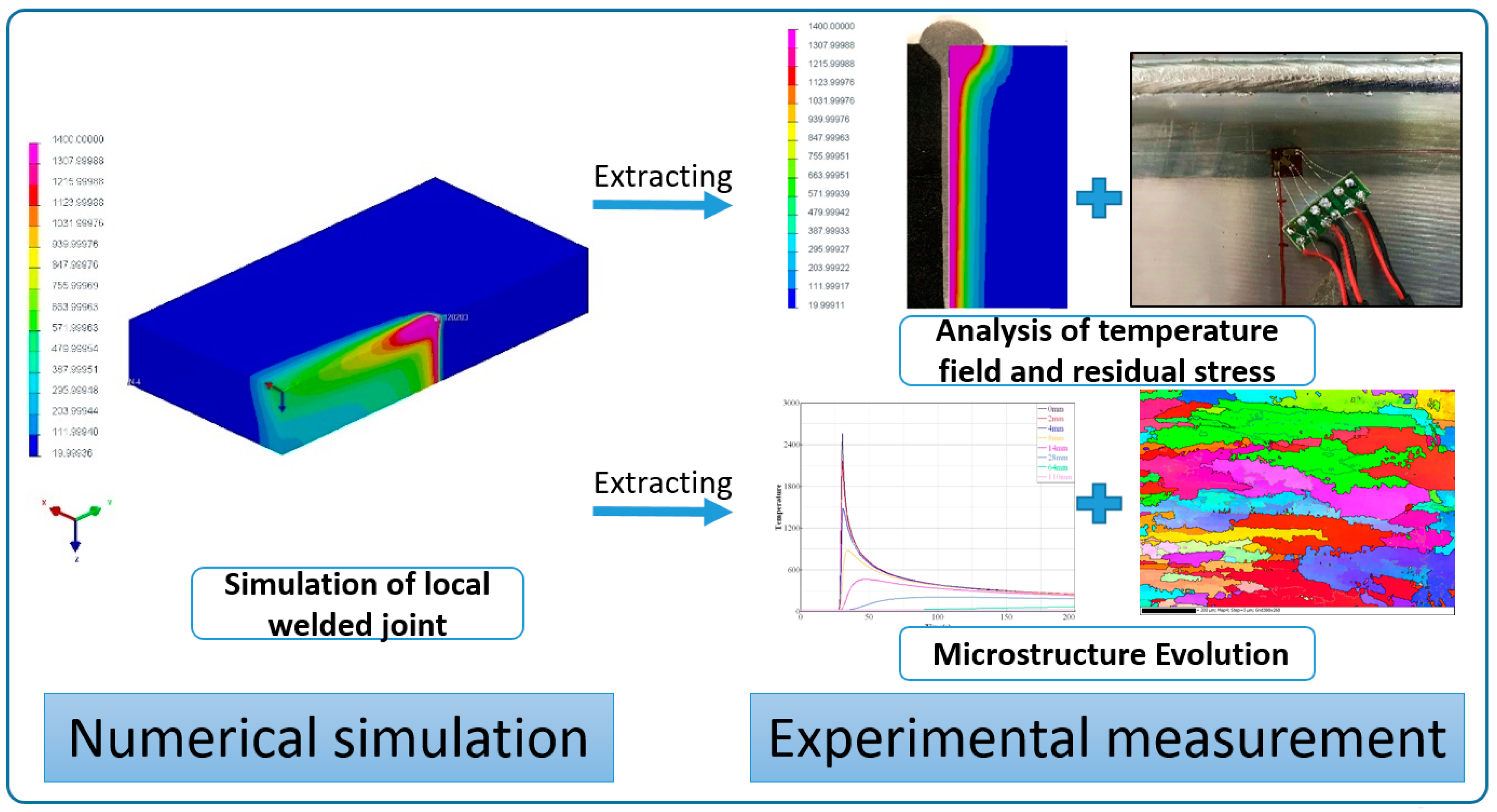
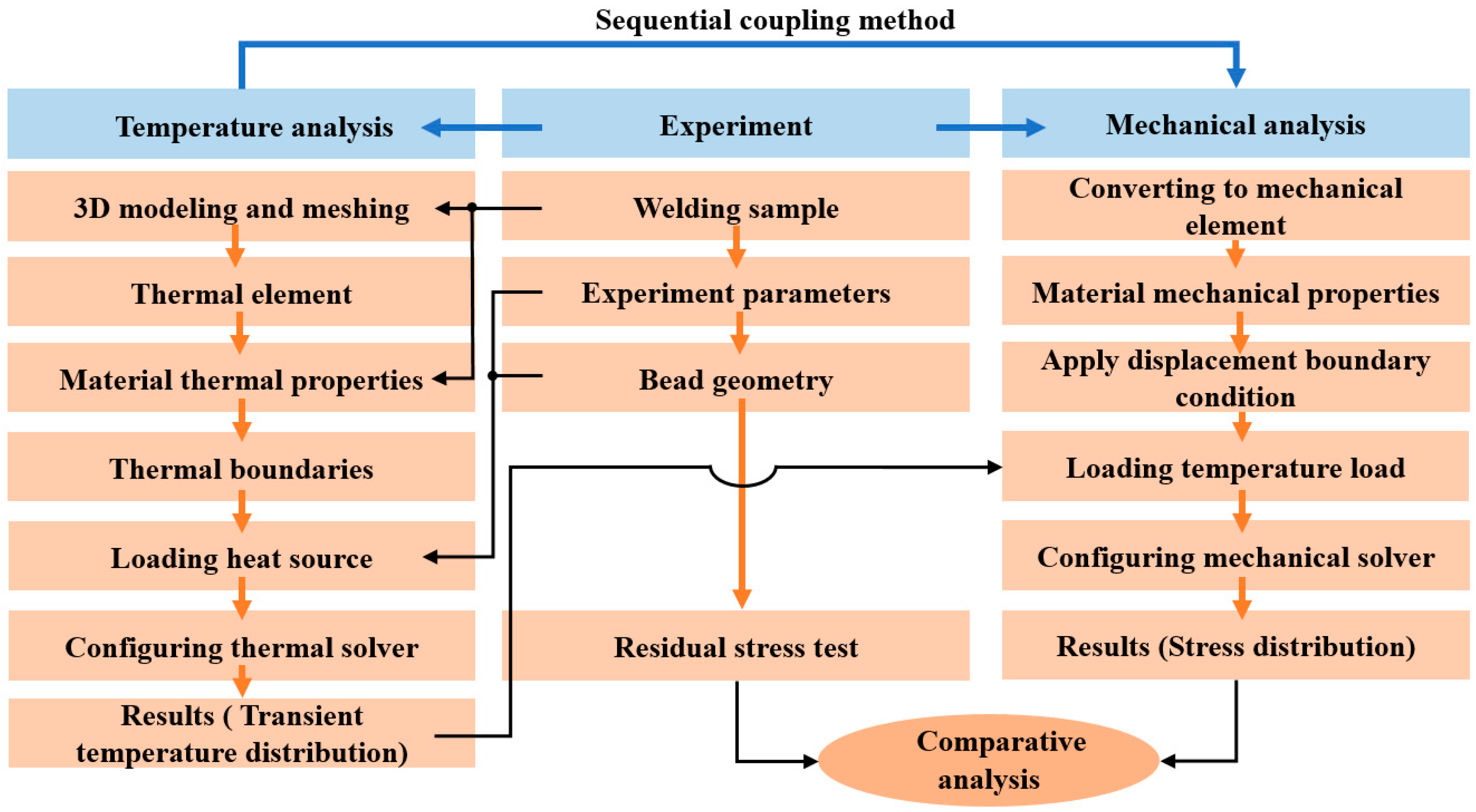
2. Methodology
3. Simulation of Local Welded Joint
3.1. The Thermal Elastoplastic Theory
3.1.1. Stress–Strain Relation
3.1.2. Balance Equation
3.1.3. Solution Procedure
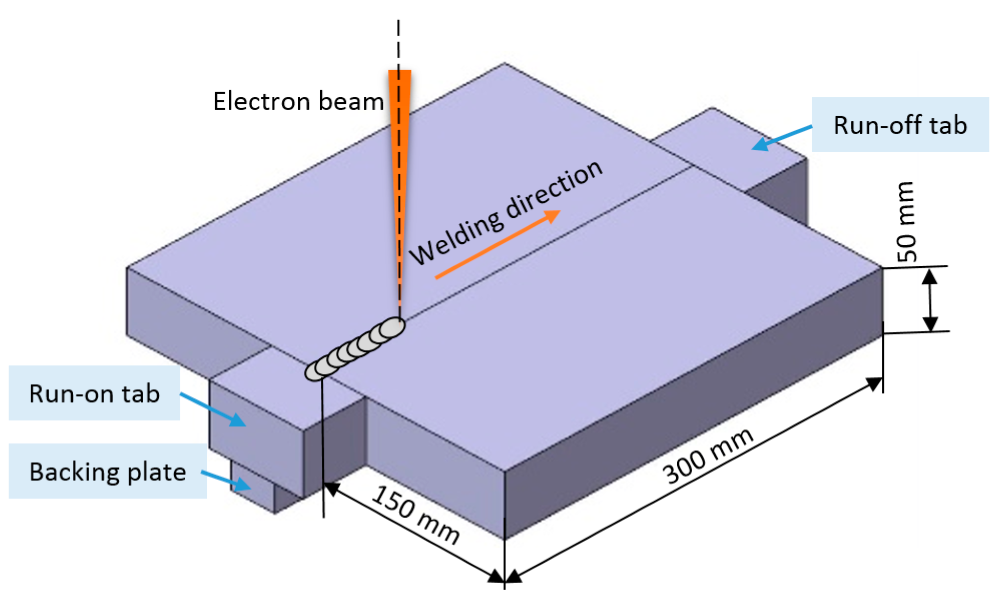
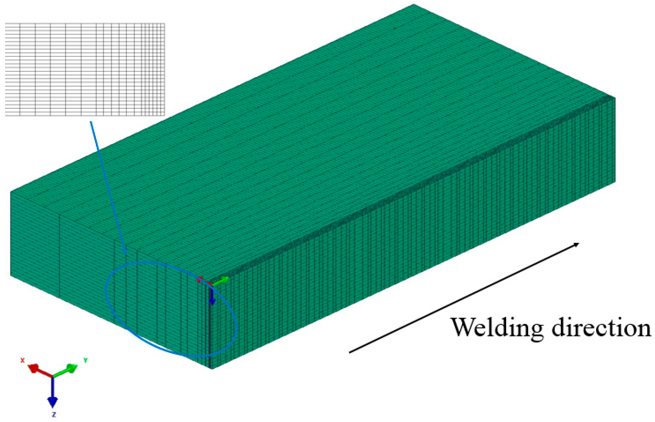
3.2. Geometry Model
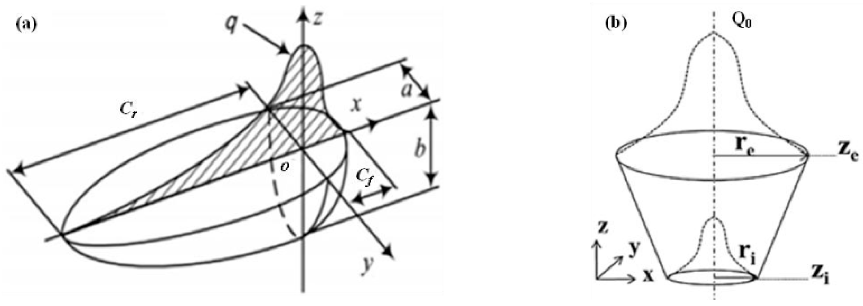
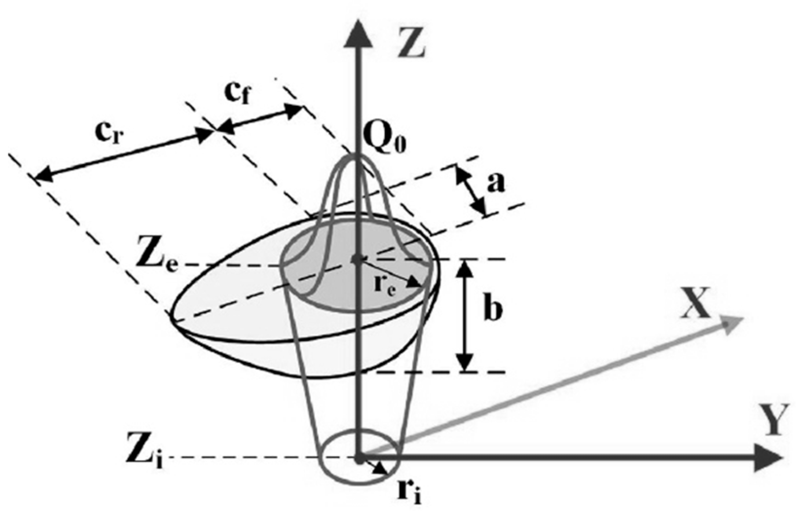
3.3. Heat Source Model
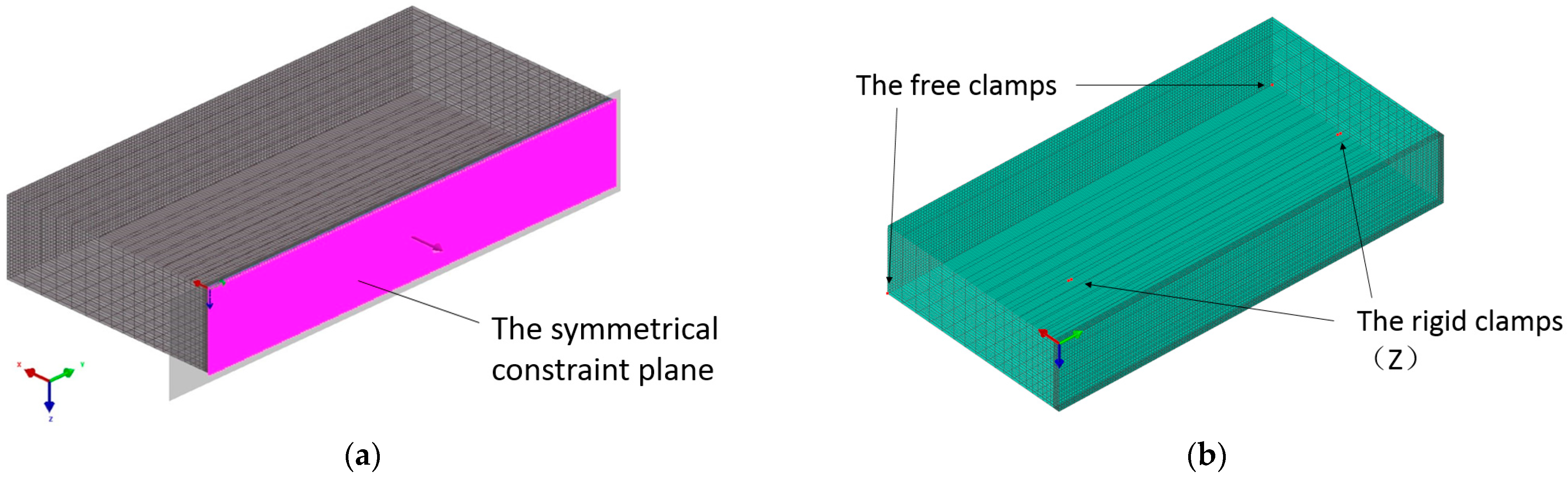
3.4. Material Properties and Boundary Condition
3.5. Simulation Result
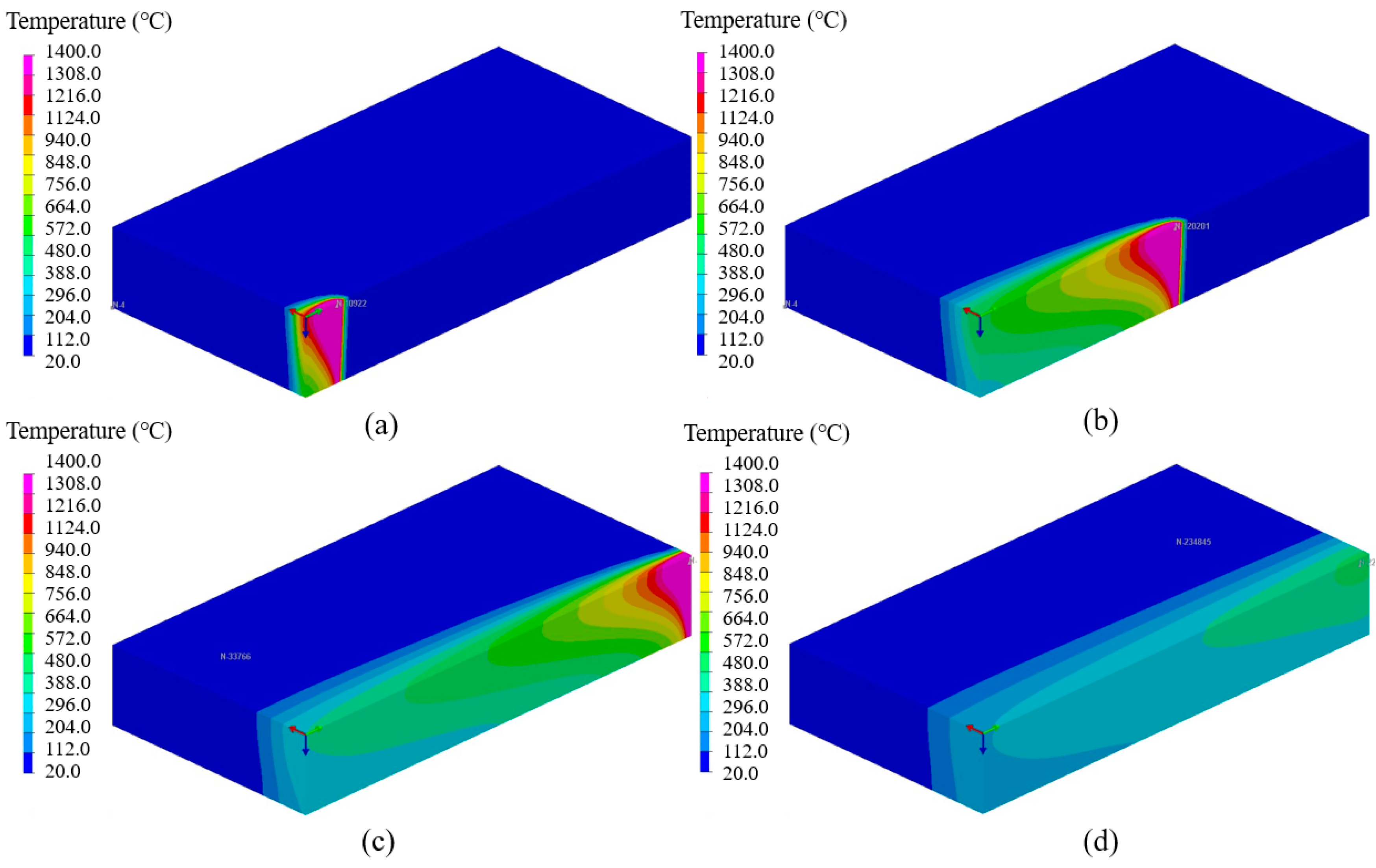
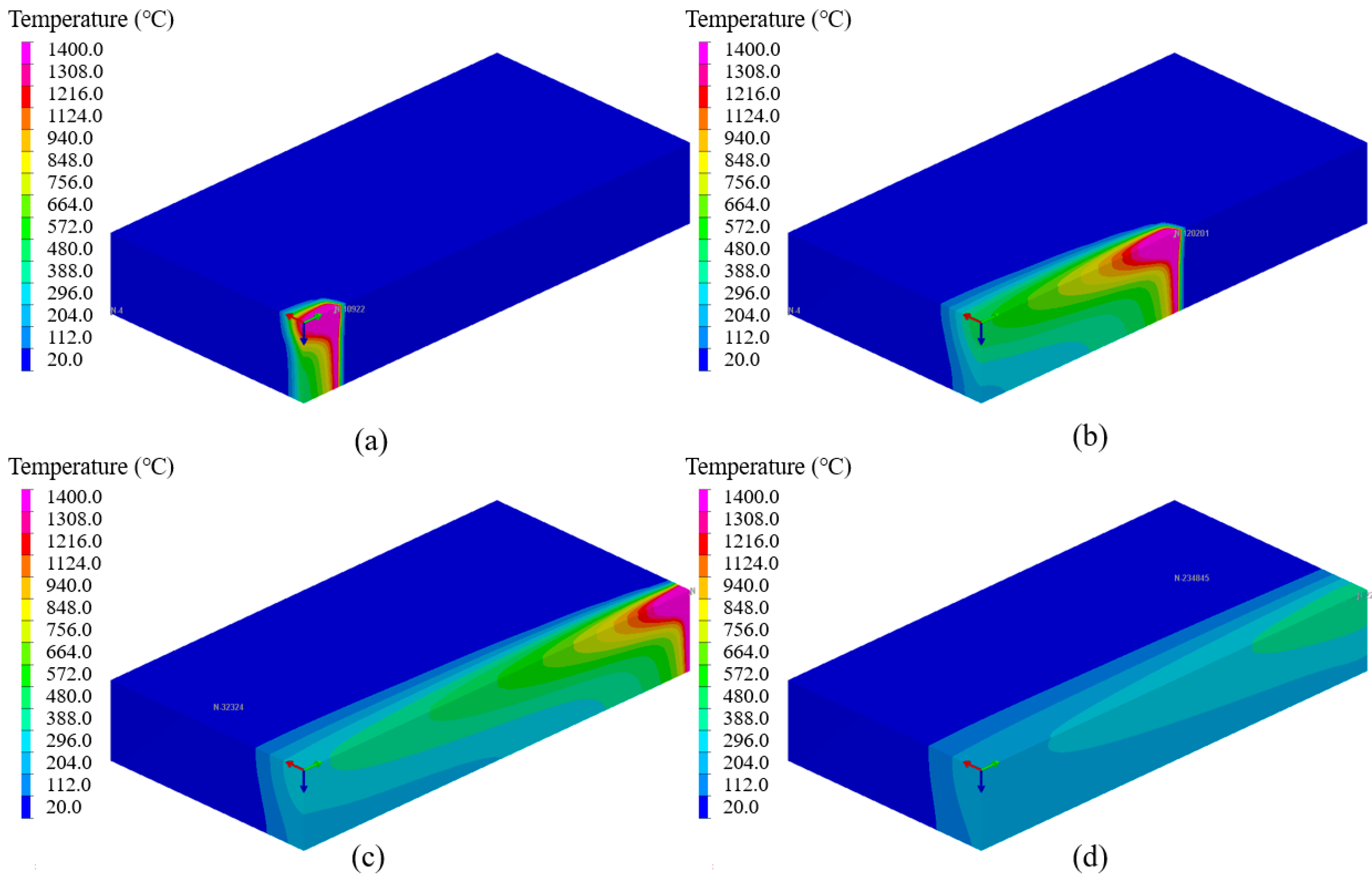
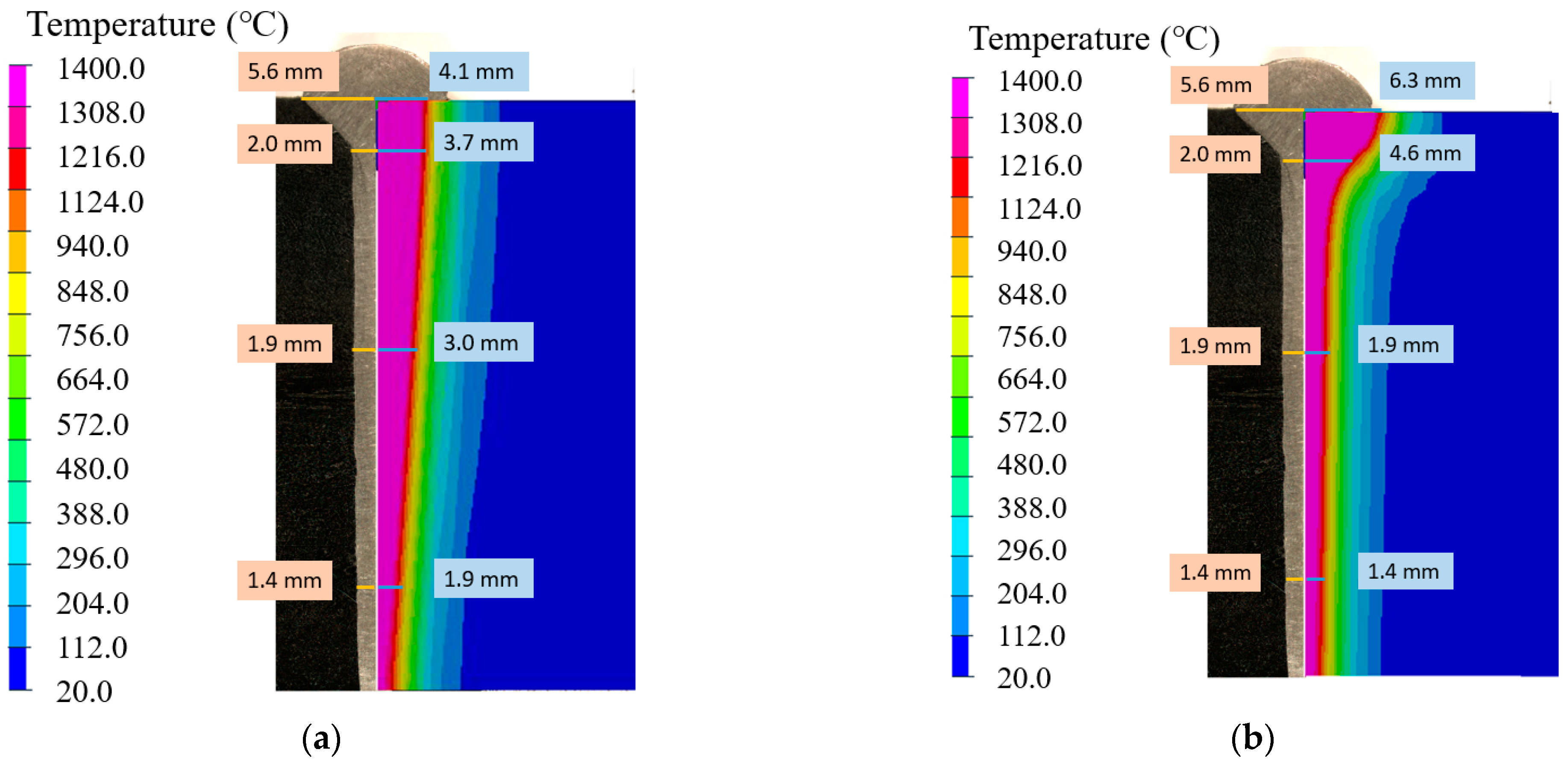
3.5.1. Temperature Field Simulation Results
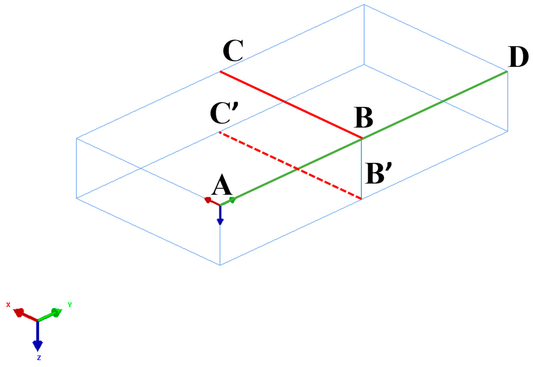
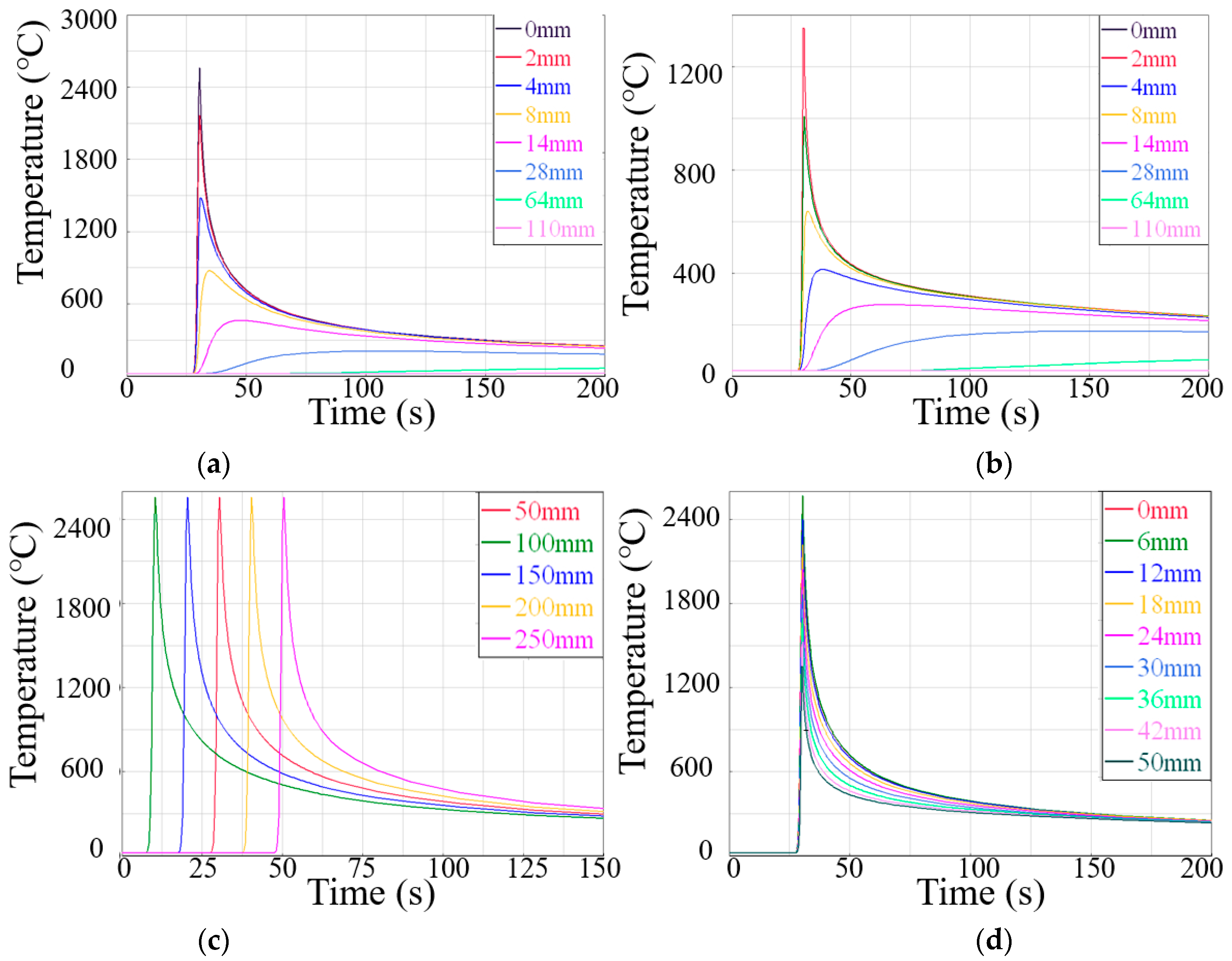
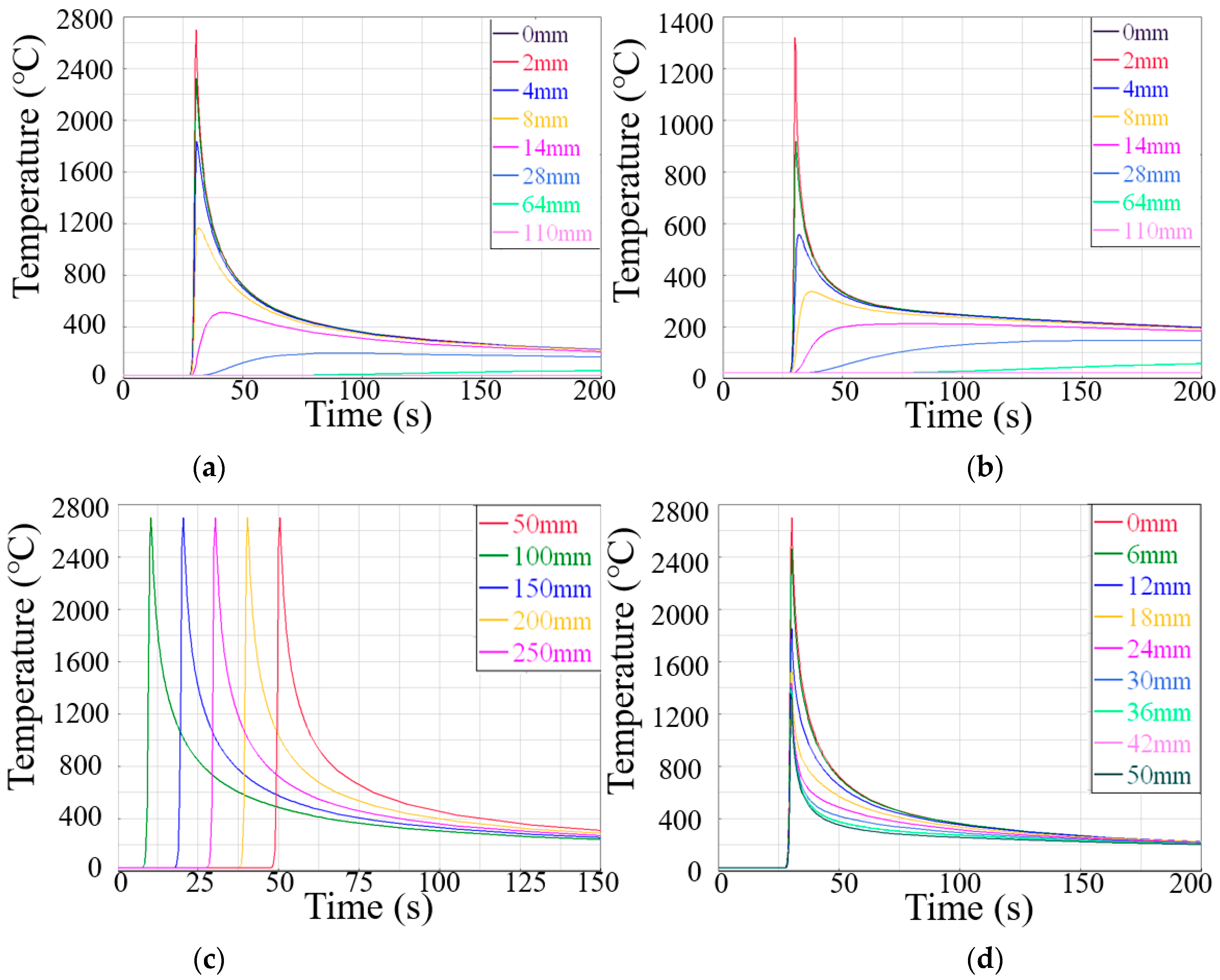
3.5.2. Extraction of Welding Thermal Cycle Curve
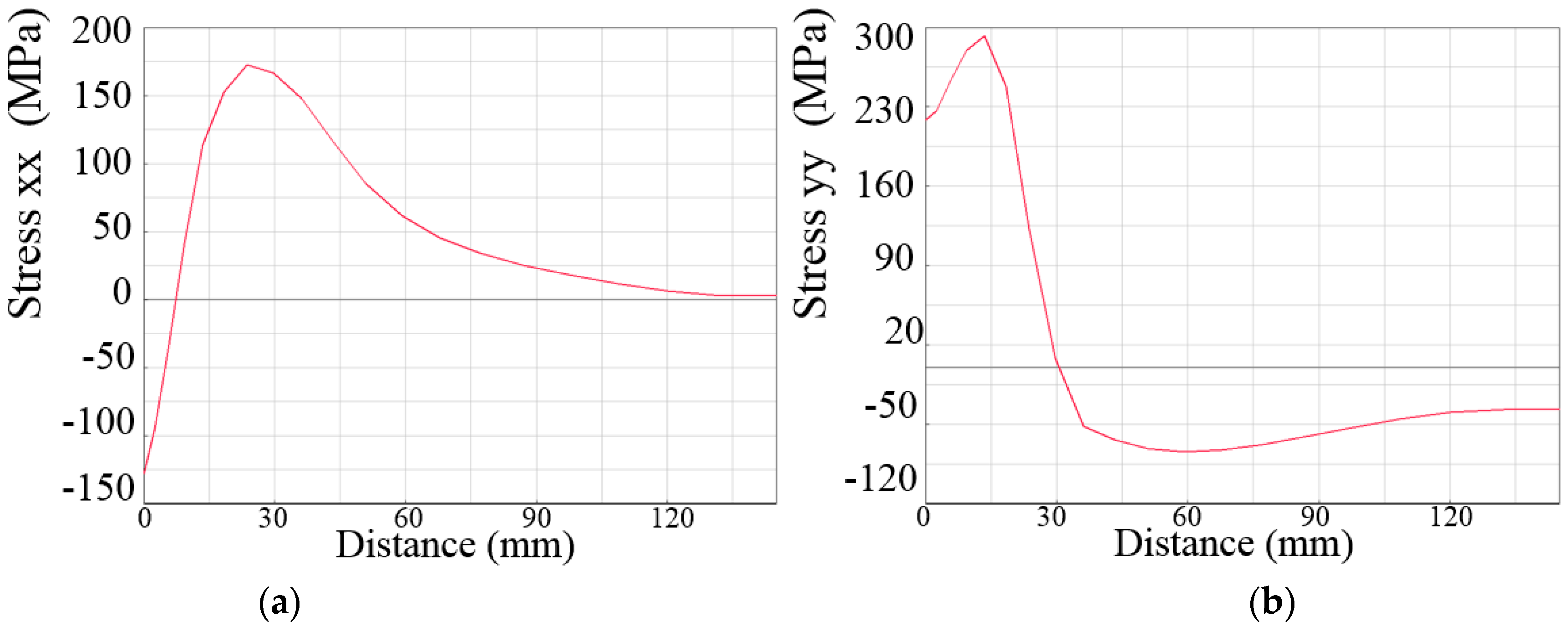
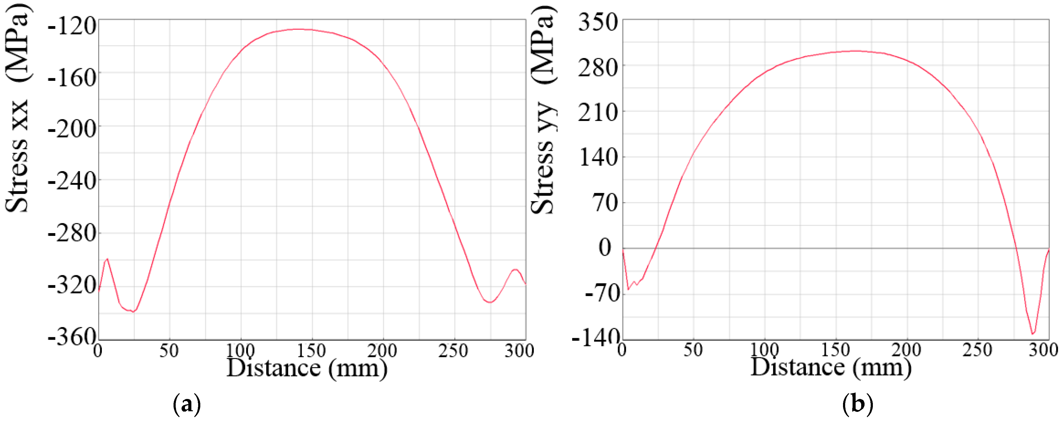
3.5.3. The Stress–Strain Field Results
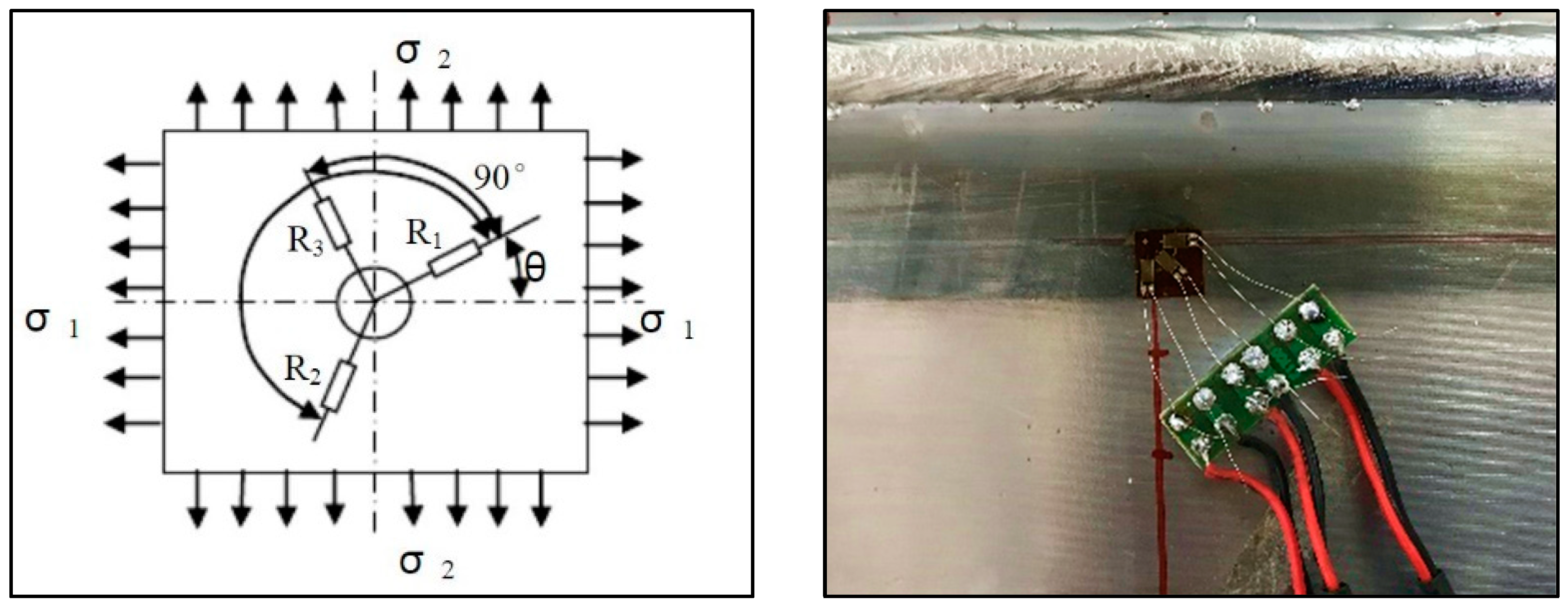
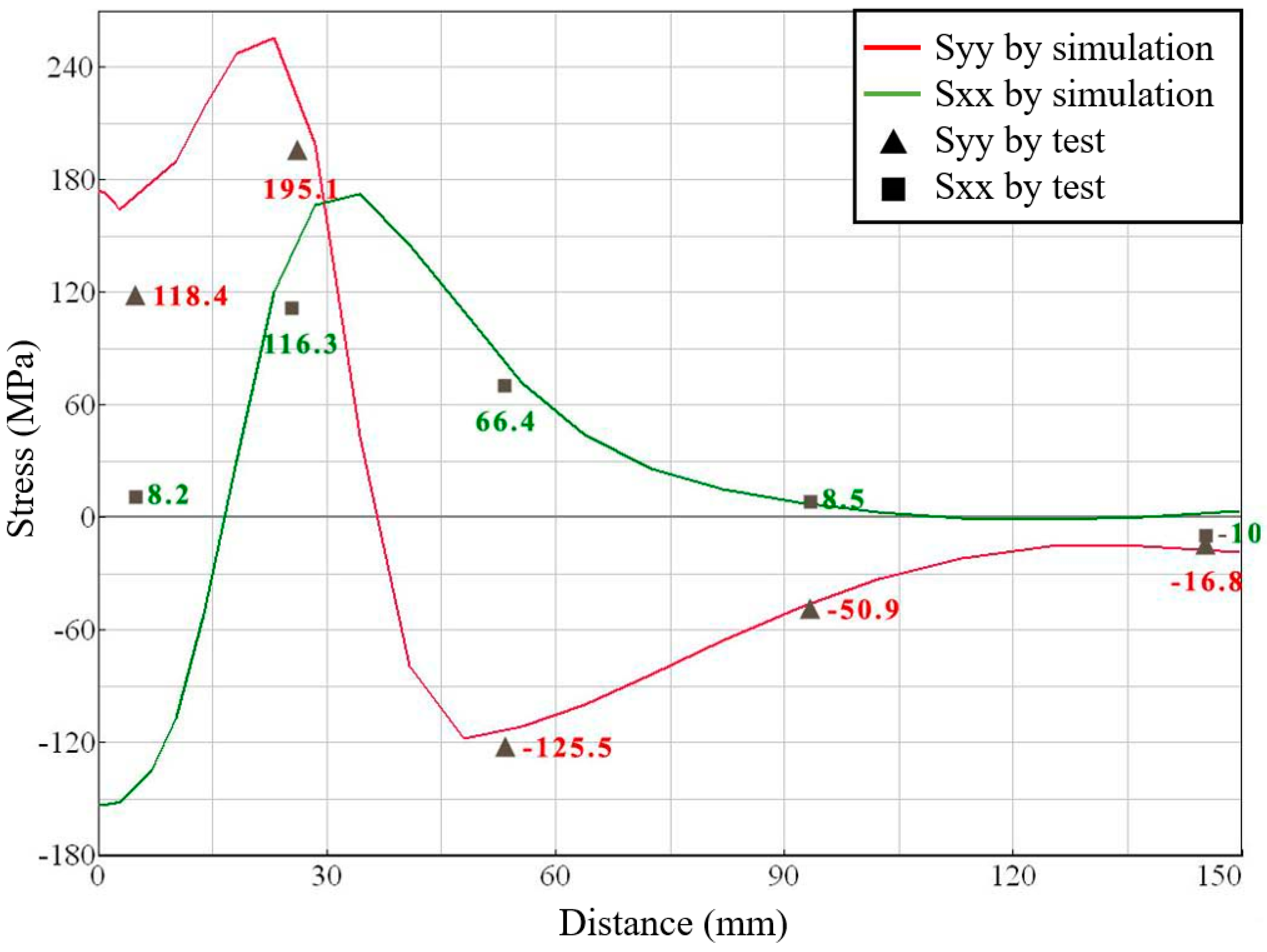
3.5.4. Welding Residual Stresses Test
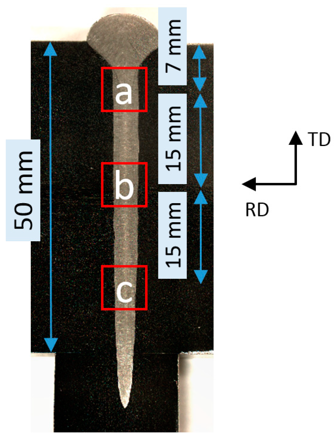
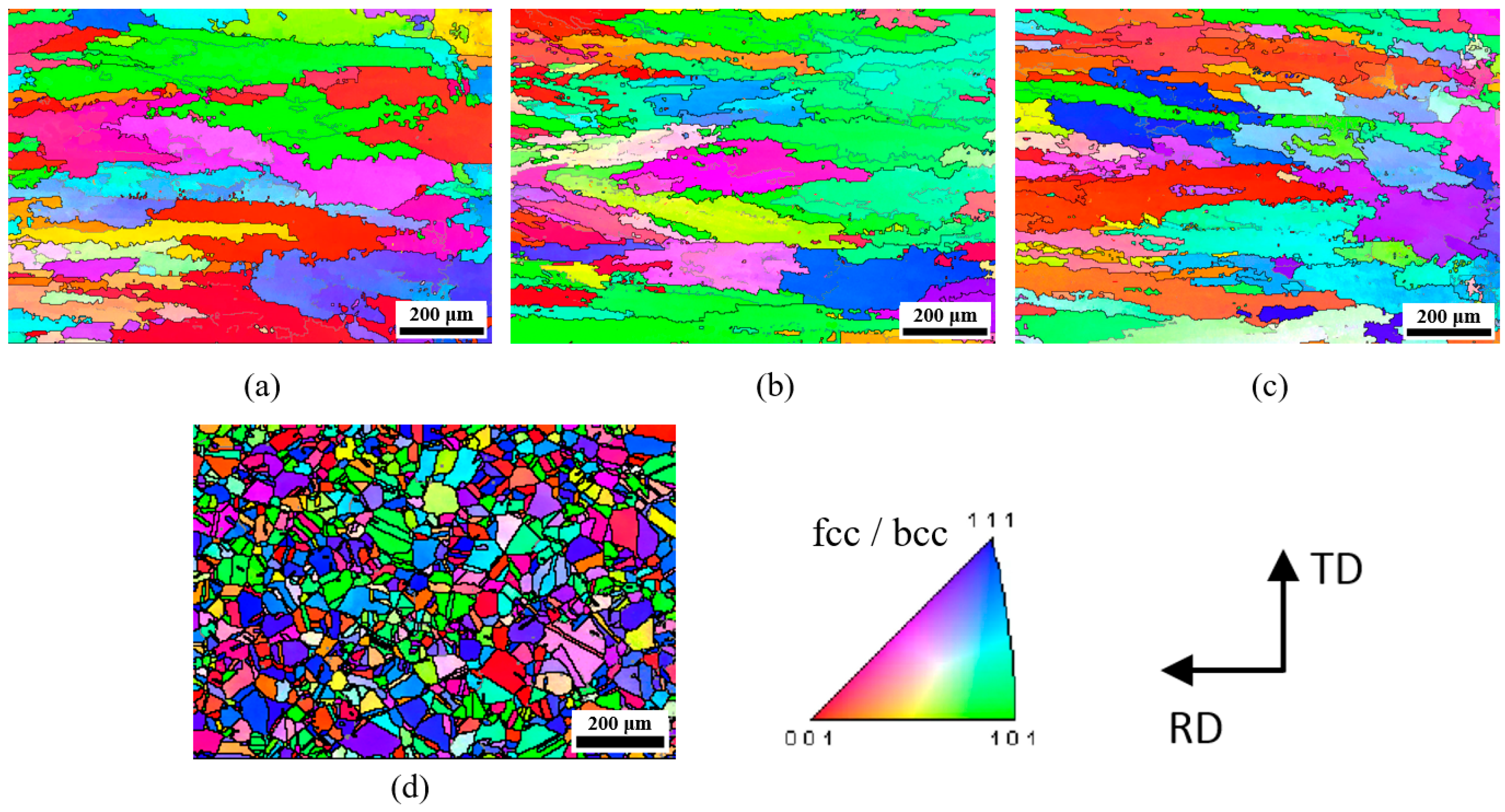
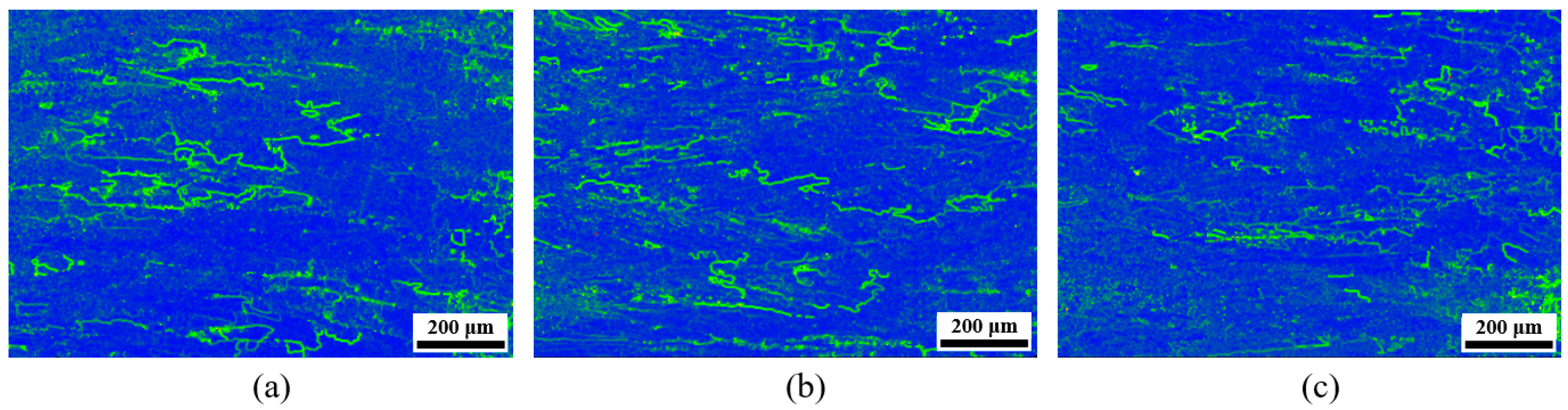
4. Mechanism Analysis of Microstructure Heterogeneity
5. Conclusions
- Compared with the 3D Gaussian heat source, the combined heat sources simulation was closer to the weld cross-section of the EBW 50 mm 316L butt welding.
- The results showed that the welding thermal cycle curves of different positions in the penetration direction are different, and EBW was a rapid heating and cooling process with the maximum heating/cooling rates of 690 °C·s−1/557 °C·s−1 during welding.
- The numerical and measurement results of the residual stresses showed a similar trend (the maximum difference of stress was 15 MPa, except for the weld center), confirming the reliability of the simulation results.
- The differences in heating and cooling rates were the main reason for the inhomogeneity of microstructure and mechanical properties. The grains of the weld turned into a group of large columnar crystals. The inhomogeneities in microstructure mainly showed that the sample at the top of the WM was easier to form stress concentration than the bottom sample.
Author Contributions
Funding
Institutional Review Board Statement
Informed Consent Statement
Data Availability Statement
Acknowledgments
Conflicts of Interest
References
- Song, Y.T.; Wu, S.T.; Li, J.G.; Wan, B.N.; Wan, Y.X.; Fu, P.; Ye, M.Y.; Zheng, J.X.; Lu, K.; Gao, X.; et al. Concept design of CFETR Tokamak machine. IEEE Trans. Plasma Sci. 2014, 42, 503–509. [Google Scholar] [CrossRef]
- Liu, Z.H.; Ji, H.B.; Wu, J.F.; Wu, H.P.; Ma, J.G.; Fan, X.S.; Wang, R.; Gu, Y.Q.; Lu, K.; Ran, H. R&D achievements for vacuum vessel towards CFETR construction. Nucl. Fusion 2020, 60, 126024. [Google Scholar]
- Ma, J.; Wu, J.F.; Liu, Z.H.; Wang, R.; Gu, Y.Q.; Fan, X.S.; Ji, H.B. Key manufacturing technologies of the CFETR 1/8 vacuum vessel sector mockup. Fusion Eng. Des. 2021, 163, 112166. [Google Scholar] [CrossRef]
- Fu, P.; Mao, Z.; Zuo, C.; Wamg, Y.; Wang, C. Microstructures and fatigue properties of electron beam welds with beam oscillation for heavy section TC4-DT alloy. Chin. J. Aeronaut. 2014, 27, 1015–1021. [Google Scholar] [CrossRef] [Green Version]
- Chen, Q.; Li, D.; He, C.; Yu, Z. Microstructure difference analysis of large thickness welded joint with EBW. Trans. China Weld. Inst. 2015, 36, 79–82. [Google Scholar]
- Xia, X.W.; Wu, J.F.; Liu, Z.H.; Ji, H.B.; Shen, X.; Ma, J.; Zhuang, P. Correlation between microstructure evolution and mechanical properties of 50 mm 316L electron beam welds. Fusion Eng. Des. 2019, 147, 111245. [Google Scholar] [CrossRef]
- Alali, M.; Todd, I.; Wynne, B.P. Through-thickness microstructure and mechanical properties of electron beam welded 20 mm thick AISI 316L austenitic stainless steel. Mater. Des. 2017, 130, 488–500. [Google Scholar] [CrossRef]
- Chiumenti, M.; Cervera, M.; Dialami, N.; Wu, B.; Li, J.; Agelet de Saracibar, C. Numerical modeling of the electron beam welding and its experimental validation. Finite Elem. Anal. Des. 2016, 121, 118–133. [Google Scholar] [CrossRef] [Green Version]
- Bonakdar, A.; Molavi-Zarandi, M.; Chiamanfar, A.; Jahazi, M.; Firoozrai, A.; Morin, E. Finite element modeling of the electron beam welding of Inconel-713LC gas turbine blades. J. Manuf. Process. 2017, 26, 339–354. [Google Scholar] [CrossRef]
- Chen, L.; Mi, G.; Zhang, X.; Wang, C. Numerical and experimental investigation on microstructure and residual stress of multi-pass hybrid laser-arc welded 316L steel. Mater. Des. 2019, 168, 107653. [Google Scholar] [CrossRef]
- Rong, Y.M.; Huang, Y.; Xu, J.J.; Zheng, H.J.; Zhang, G.J. Numerical simulation and experiment analysis of angular distortion and residual stress in hybrid laser-magnetic welding. J. Mater. Process. Technol. 2017, 245, 270–277. [Google Scholar] [CrossRef]
- Ueda, Y.; Yamakawa, T. Analysis of thermal elastic-plastic stress and strain during welding by finite element method. Trans. Jpn. Weld. Soc. 1971, 2, 186–196. [Google Scholar]
- Bang, H.S. Transient Thermal Analysis of Friction Stir Welding using 3D-Analytical Model of Stir Zone. J. Weld. Join. 2008, 12, 36–41. [Google Scholar] [CrossRef] [Green Version]
- Wang, J.; Ueda, Y.; Murakawa, H.; Yang, H.Q.; Yuan, M.G. Improvement in numerical accuracy and stability of 3-D FEM analysis in welding. Weld. J. 1996, 75, 129s–134s. [Google Scholar]
- Xu, J.; Chen, C.; Lei, T.; Wang, W.; Rong, Y. Inhomogeneous thermal-mechanical analysis of 316L butt joint in laser welding. Opt. Laser Technol. 2019, 115, 71–80. [Google Scholar] [CrossRef]
- Zhang, H.; Men, Z.X.; Li, J.K.; Liu, Y.J.; Wang, Q.Y. Numerical simulation of the electron beam welding and post welding heat treatment coupling process. High Temp. Mater. Proc. 2018, 37. [Google Scholar] [CrossRef]
- Chukkana, J.R.; Vasudevanb, M.; Muthukumarana, S.; Kumar, R.R.; Chandrasekhar, N. Simulation of laser butt welding of AISI 316L stainless steel sheetusing various heat sources and experimental validation. J. Mater. Process. Technol. 2015, 219, 48–59. [Google Scholar] [CrossRef]
- Xin, J.J. Mechanism of Weld Forming and Deformation Control of ITER Correction Coil BCC Case. Ph.D. Thesis, University of Science and Technology of China, Hefei, China, 2019. [Google Scholar]
- Xiu, L. Welding Simulation of Large Heavy-Load Complex Contour Vacuum Vessel and Study on Method to Releve Residual Stress. Ph.D. Thesis, University of Science and Technology of China, Hefei, China, 2017. [Google Scholar]
- Yang, J.; Dong, H.G.; Xia, Y.Q.; Li, P.; Ma, Y.T.; Wu, W.; Wang, B.S. The microstructure mechanical properties of novel cryogenic twinning-induced plasticity steel welded joint. Mater. Sci. Eng. A 2021, 818, 141449. [Google Scholar] [CrossRef]
- Ding, C.; Liu, J.L.; Guan, Y.Z.; Mi, X.C.; Ji, S.K.; Wang, G.D. EBSD analysis of weldment microstructure based on blast furnace hull. Res. Explor. Lab. 2012, 31, 290–295. [Google Scholar]


| Element | Cr | Ni | Mo | Mn | Si | Cu | P | C | N | S | Fe |
|---|---|---|---|---|---|---|---|---|---|---|---|
| wt% | 16.31 | 10.12 | 2.04 | 1.36 | 0.50 | 0.3 | 0.032 | 0.012 | 0.027 | 0.004 | rest |
| Voltage Ua (kV) | Beam Current Ib (mA) | Focusing Lens Current If (mA) | Velocity v (mm/s) | Working Distance (mm) | Welding Attitude | Working Pressure of the Electron Beam Machine Chamber (mbar) |
|---|---|---|---|---|---|---|
| 150 | 140 | 2407 | 5 | 440 | horizontal | 1.7 × 10⁻⁴ |
| Temperature (°C) | Thermal Conductivity | Specific Heat (J/g·K) | Density (kg/m3) | Coefficient of Thermal Expansion (10−6 mm/K) | Elastic Modulus (GPa) | Poisson’s Ratio | Yield Strengths (MPa) | Tensile Strengths Limit (MPa) (1% Strain) |
|---|---|---|---|---|---|---|---|---|
| 20 | 13.31 | 0.470 | 7966 | 15.24 | 195.1 | 0.267 | 278 | 325 |
| 200 | 16.33 | 0.508 | 7893 | 16.43 | 185.7 | 0.290 | 193 | 226 |
| 400 | 19.47 | 0.550 | 7814 | 17.44 | 172.6 | 0.322 | 154 | 180 |
| 600 | 22.38 | 0.592 | 7724 | 18.21 | 155.0 | 0.296 | 141 | 165 |
| 800 | 25.07 | 0.634 | 7630 | 18.83 | 131.4 | 0.262 | 130 | 153 |
| 900 | 26.33 | 0.655 | 7583 | 19.11 | 116.8 | 0.24 | 86 | 100 |
| 1000 | 27.53 | 0.676 | 7535 | 19.38 | 100.1 | 0.229 | 45 | 53 |
| 1100 | 28.67 | 0.698 | 7486 | 19.66 | 81.1 | 0.223 | 22 | 23 |
| 1200 | 29.76 | 0.719 | 7436 | 19.95 | 59.5 | 0.223 | 13 | 15 |
| 1420 | 31.95 | 0.765 | 7320 | 20.7 | 2.0 | 0.223 | 3 | 3.3 |
| 1460 | 320 | 0.765 | 7320 | 20.7 | 2.0 | 0.223 | 3 | 3.3 |
Publisher’s Note: MDPI stays neutral with regard to jurisdictional claims in published maps and institutional affiliations. |
© 2022 by the authors. Licensee MDPI, Basel, Switzerland. This article is an open access article distributed under the terms and conditions of the Creative Commons Attribution (CC BY) license (https://creativecommons.org/licenses/by/4.0/).
Share and Cite
Xia, X.; Wu, J.; Liu, Z.; Ma, J.; Ji, H.; Lin, X. Numerical Simulation of 50 mm 316L Steel Joint of EBW and Its Experimental Validation. Metals 2022, 12, 725. https://doi.org/10.3390/met12050725
Xia X, Wu J, Liu Z, Ma J, Ji H, Lin X. Numerical Simulation of 50 mm 316L Steel Joint of EBW and Its Experimental Validation. Metals. 2022; 12(5):725. https://doi.org/10.3390/met12050725
Chicago/Turabian StyleXia, Xiaowei, Jiefeng Wu, Zhihong Liu, Jianguo Ma, Haibiao Ji, and Xiaodong Lin. 2022. "Numerical Simulation of 50 mm 316L Steel Joint of EBW and Its Experimental Validation" Metals 12, no. 5: 725. https://doi.org/10.3390/met12050725
APA StyleXia, X., Wu, J., Liu, Z., Ma, J., Ji, H., & Lin, X. (2022). Numerical Simulation of 50 mm 316L Steel Joint of EBW and Its Experimental Validation. Metals, 12(5), 725. https://doi.org/10.3390/met12050725