Abstract
Recently, the development of β-titanium (Ti) alloys with a low Young’s modulus as human implants has been the trend of research in biomedical materials. However, designing β-titanium alloys by conventional experimental methods is too costly and inefficient. Therefore, it is necessary to propose a method that can efficiently and reliably predict the microstructures and the mechanical properties of biomedical titanium alloys. In this study, a machine learning prediction method is proposed to accelerate the design of biomedical multi-component β-Ti alloys with low moduli. Prediction models of microstructures and Young’s moduli were built at first. The performances of the models were improved by introducing new experimental data. With the help of the models, a Ti–13Nb–12Ta–10Zr–4Sn (wt.%) alloy with a single β-phase microstructure and Young’s modulus of 69.91 GPa is successfully developed. This approach could also be used to design other advanced materials.
1. Introduction
Titanium (Ti) alloys are widely used in biomedical applications, such as bone-fixation devices, owing to their excellent biocompatibility, corrosion resistance, low density, and superior overall mechanical properties [1,2]. The Ti–6Al–4V (wt.%) alloy has long been used as a human implant material. However, the Young’s modulus of Ti–6Al–4V (110 GPa) is much higher than the modulus of human bone (<35 GPa). The differences in Young’s modulus between alloys and bones could lead to the stress shielding effect and degradation of bones [3]. Moreover, aluminum and vanadium elements are not ideal for human implantations, because they are cytotoxic and could cause a range of physiological disorders with long-term exposure to the physiological environment [4,5]. In the last several years, some researchers found that β-Ti alloys have high strength, excellent biocompatibility, and low Young’s modulus, in comparison to α-Ti (e.g., pure Ti) or α + β-Ti (e.g., Ti-6Al-4V), which could have significant potential in biomedical applications [6,7]. However, it has been generally accepted that it is difficult to achieve an excellent synergy between low modulus and phase stability in β-Ti alloys. Moreover, the complex mechanism of the influence of alloy elements on Young’s modulus is also a challenge when designing new alloys.
Therefore, a large number of studies have attempted to improve the alloys. Most of these studies are based on experimental methods [8,9,10]. Moreover, some researchers have tried to design alloys by empirical calculation methods, such as the molybdenum equivalence () [11,12,13] and d-electron theory [14,15]. Computational material methods (including CALPHAD [16,17], the density functional theory (DFT) [18,19], and molecular dynamics (MDs) [20,21]) are also used. However, these methods are inefficient or require high computational resources. In this case, it necessary to find a new approach that can accurately and efficiently predict the Young’s modulus of alloys.
Recently, with the development of artificial intelligence, machine learning has been widely used in various fields. In materials science, machine learning is used to establish influence factors (features)–property relationship to solve different challenges, such as multiple property designs [22,23,24,25,26,27,28]. The properties of metallic materials could be modeled using machine learning, which accelerates the design and development of novel materials. Honysz [29] modeled artificial neural networks and successfully predicted the chemical composition of ferritic stainless steels for corresponding mechanical properties. Churyumov et al. [30] modeled an artificial neural network to analyze how alloying element concentrations influenced the behavior of hot deformation. Machine learning could also be used for β-Ti alloys, for which the moduli are close to the moduli of human bones. For instance, relationships between the compositions and Young’s moduli of the β-Ti alloys were built in the studies of Yang et al. [31] and Wu et al. [32]. Low-modulus β-Ti alloys that have a Young’s modulus less than 50 GPa were designed with the help of their machine learning models. In their studies, however, the compositions of the alloys were regarded as the only features. Other important features (such as the solution temperature, solution time, and mixing enthalpy) were not considered in their study. Furthermore, some researchers used machine learning to find features that could describe the Young’s moduli of β-Ti alloys more exhaustively. Xiong et al. [33] discovered four critical features that strongly affected the energetic stability and Young’s modulus in the binary Ti–Zr system. However, their results are not suitable for multi-component β-Ti alloy systems.
To solve the problems mentioned above, a machine learning method is proposed in the present study, to predict the microstructures and Young’s moduli of the biomedical multi-component β-Ti alloys. Furthermore, new features embedded with the knowledge of the domain materials of alloys are established. A classification model is built to predict whether the alloy is composed of single β-phase or not, while a regression model is built to predict the Young’s modulus. These two models are modified by introducing new experimental data. Finally, the accuracies of the models reach a high level, which could be of vital use for the design of biomedical multi-component β-Ti alloys.
2. Materials and Methods
2.1. Approach
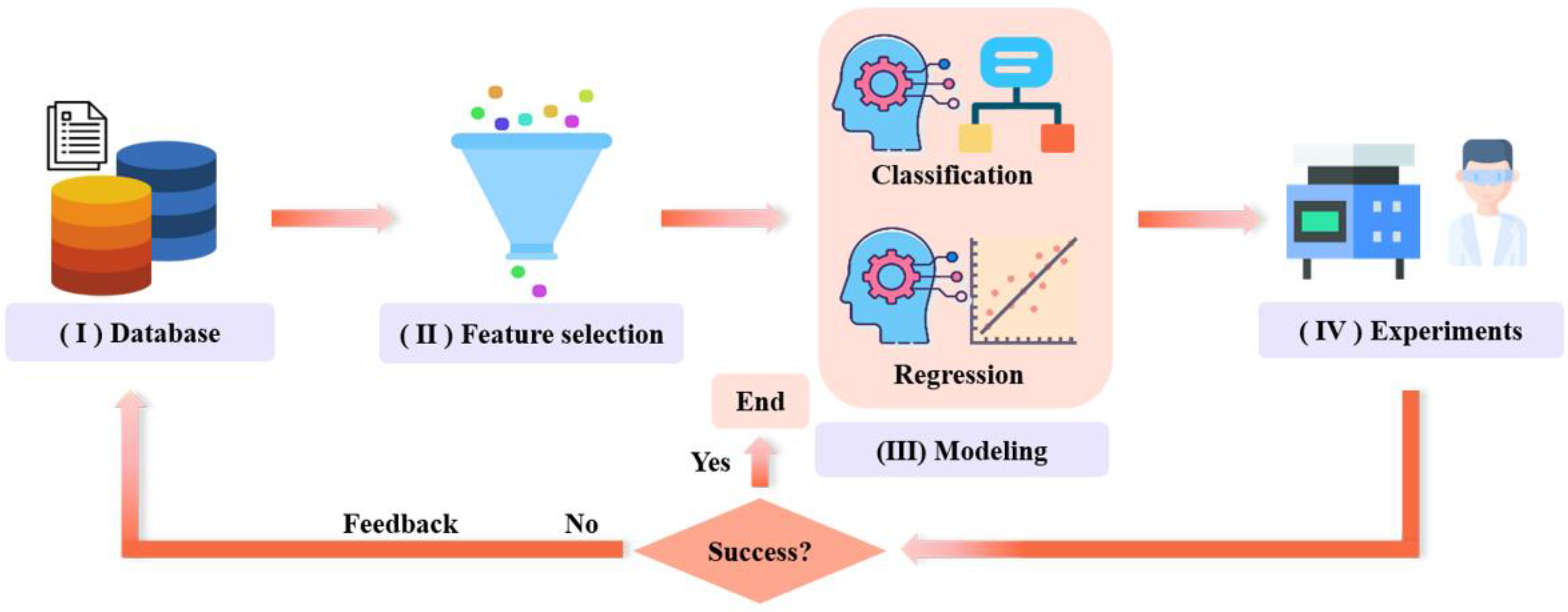
A machine learning prediction method was proposed to predict the microstructures and Young’s moduli of the biomedical multi-component β-Ti alloys, as shown in Figure 1. The method was composed of four main steps: (1) data collection; (2) feature selection; (3) model building; and (4) experiments.

Figure 1.
A machine learning prediction method to predict the microstructures and Young’s moduli of the biomedical multi-component β-Ti alloys.
- (1)
- Collecting biomedical Ti alloys data reported in the relevant literature as machine learning databases were used for the training and testing of models.
- (2)
- It is difficult to interpret the prediction results only considering the chemical compositions as features for machine learning. The interpretability and robustness of the model could be improved by embedding the material domain knowledge into the machine learning. Some features were suggested, including heat-treatment process parameters, and macroscopic as well as microscopic properties. Following the feature selection method, the most relevant features were retained.
- (3)
- A classification model and a regression model were built. The classification model was utilized to predict the microstructures, and the regression model was utilized to predict Young’s modulus. It is worth noting that there were many hyperparameters to optimize the modeling process. The Bayesian optimization algorithm was used to automatically find the hyperparameters. The optimized hyperparameters were then subjected to machine learning training.
- (4)
- Once the models were built, the microstructures and Young’s modulus of the β-Ti alloys could be predicted in the virtual space of the compositions and heat-treatment process. To validate the performances of the models, the multi-component Ti alloys were prepared. Subsequently, the observation of the microstructures and mechanical property test were performed. Finally, the experimental results were fed back into the machine learning databases for the next iteration and design.
2.2. Datasets
Two datasets, the microstructure and Young’s modulus datasets, were collected from the relevant literature reports and used to train the classification and regression models, respectively. All the data were carefully selected. The records with errors and data with low reliability were not included. Finally, we collected 342 different alloy compositions and 235 Young’s moduli with different β-Ti alloy compositions. In the Young’s modulus dataset, all the alloys were single β-phase alloys prepared by the quenching process, with only minor amounts of α″ and ω phases permitted. Each dataset was randomly divided into training and testing datasets in the ratio of 7:3. The training dataset was used to train the model, and the testing dataset was used to test the model’s performance.
Embedding the physical and chemical properties of materials as features into the machine learning model could provide a priori knowledge to improve the model’s performance and interpret the predictions [34,35,36]. Thus, we examined some physical and chemical property parameters that potentially influenced the microstructures and Young’s modulus of Ti alloys. The features included alloy compositions, solution temperature, solution time, molybdenum equivalence (), the average valence electron concentration (), the average density (), the average bulk modulus () and the average bulk modulus (), as seen in Table 1.

Table 1.
A total of 33 features used to build the machine learning models.
Table 1.
A total of 33 features used to build the machine learning models.
| Features | Formula | Range | Description |
|---|---|---|---|
| Ti | - | 30~92 | mass% |
| Nb | - | 0~45 | mass% |
| Sn | - | 0~14 | mass% |
| Mo | - | 0~20 | mass% |
| Zr | - | 0~41 | mass% |
| Ta | - | 0~16 | mass% |
| Cr | - | 0~14 | mass% |
| Mn | - | 0~18 | mass% |
| Temp | - | Solution temperature | |
| Time | - | Solution time | |
| Atomic weight [37] | |||
| Density [37] | |||
| Metallic radius [37] | |||
| Heat of fusion [38] | |||
| Heat of vaporization [38] | |||
| Specific heat [38] | |||
| Melting point [37] | |||
| Bulk modulus [38] | |||
| Shear modulus [38] | |||
| Young’s modulus [38] | |||
| Thermal conductivity [37] | |||
| Lattice volume [37] | |||
| Valence electrons [39] | |||
| Difference of atomic radii [37] | |||
| Pauling electronegativity [37] | |||
| Mixing enthalpy [37] | |||
| Mixing entropy [37] | |||
| Free energy of mixing [37] | |||
| Ω parameter [37] | |||
| Molybdenum equivalence [40] | |||
| Effective nuclei charges [41] | |||
| Bond order [41] | |||
| d-orbital energy level [41] | |||
| Bonding | Approximate interatomic bonding force [41] |
Note: , , , , , , , , , , , , , , , , , and represent the mass fraction; atomic weight; density; metal radius; heat of fusion; heat of vaporization; specific heat; melting point; bulk modulus; shear modulus; elastic modulus; thermal conductivity; lattice volume; valence electrons; atomic radius; bond order; transition metal; and effective nuclei charges of element i, respectively. represents the mixing enthalpy of elements i and j.
Machine learning algorithms calculate the Euclidean distance between data points. Each data point is different in magnitude, unit, and range. Hence, all the features are normalized, so that they reach the same magnitude, and are scaled to the interval (0,1), according to formula (1):
where is the normalized processed dataset, is the initial dataset, is the maximum value of the initial dataset and is the minimum value of the initial dataset.
2.3. Feature Selection
The feature selection method is an essential part of the “data preprocessing” process in machine learning. The performance of the model can be adversely impacted by irrelevant and redundant features. Using feature selection to remove these features, the prediction capability and robustness of the model can be improved. Currently, the most popular feature reduction methods are filter, wrapper and embedded methods [42]. The wrapper method finds the optimal subset of candidate features at the cost of computation. In comparison to the other two methods, the wrapper method is highly accurate and efficient. In the present study, the forward sequential feature selection (FSS), one of the wrapper methods, was used to maximize the prediction accuracy. The implementation details are as follows:
- (1)
- Create an empty subset of features.
- (2)
- Randomly insert a new feature into the previous subset of features. The newly inserted feature can be kept as part of the subset of features, if it improves the performance of the model.
- (3)
- Repeat (2) until no more features are available to be inserted into the subset of features.
- (4)
- Keep repeating processes (1)–(3) until no more optimal subsets of the features are found.
With the FSS method, the most optimal feature subset could be selected to maximize the performance of the model.
2.4. Model Building
2.4.1. Classification Models
To predict the microstructures, seven classification models were used: light gradient-boosting machine classification (LGBMC), extreme gradient-boosting classification (XGBC), gradient-boosting decision-tree classification (GBDTC), random forest classification (RFC), support vector machine based on linear (SVC.l) and Gaussian kernels (SVC.r), and K-Nearest Neighbors (KNN). Accuracy (accuracy) is used as a metric to assess the performance of the classification model. The closer the value is to 1, the better the ability of the model to identify the β-phase and non-β-phase, see formula (2). The ROC curve is also used to evaluate the generalization ability of the classification model. The area value under the ROC curve, or AUC, is calculated to indicate the performance of the classification model.
where True Positive and True Negative indicate actual β-phase alloy, predicted β-phase alloy and non-β-phase alloy, respectively; False Positive and False Negative indicate actual not β-phase alloy, predicted β-Ti alloy and non-β-Ti alloy, respectively.
2.4.2. Regression Models
To predict the Young’s modulus, seven regression models, light gradient-boosting machine regression (LGBMR), extreme gradient-boosting regression (XGBR), gradient-boosting decision-tree regression (GBDTR), random forest regression (RFR), support vector machine based on linear (SVR.l) and Gaussian kernels (SVR.r), and ElasticNet (ENET) were used. The root-mean-square error (RMSE) and R-squared coefficients () were chosen for the evaluation metrics. The RMSE was used to measure the average difference between the predicted and true values of the model, as shown in formula (3). The coefficient reflects the extent to which the variation in Young’s modulus can be explained by the features, as calculated in formula (4). Its value ranges from 0 to 1. As approaches 1, the better the fit of the regression.
where denotes the experimentally measured Young’s modulus, denotes the predicted Young’s modulus and N denotes the size of the dataset.
2.4.3. K-Fold Cross Validation
Cross validation was used to evaluate the machine learning performance. The dataset was randomly divided into k subsets. The k-1 of these subsets was used as the training of the model and the remaining subsets were used as the testing of the model. This resulted in k-division cases. Finally, the performance of the model was evaluated by averaging the evaluation results of the k-testing cases. Generally, there was no definite value of k [43]. In this work, the value of k was taken as 5.
2.4.4. Hyperparameter Optimization
Machine learning algorithms have many hyperparameters to be optimized in the modeling process. The grid search is the most widely used hyperparameter search algorithm. The optimal value was determined by finding all the points in the search range. However, grid search is resource intensive, especially when many hyperparameters have to be tuned. Thus, in the current work, Bayesian optimization was used to accelerate the hyperparameter tuning process. In comparison to grid search, Bayesian optimization uses a Gaussian process that takes into account a priori parameter information. This process continuously updates the optimization, significantly reducing the number of computational iterations.
2.4.5. Modeling Method
In this study, the computational methods described above were implemented using the Python3 language. Scikit-learn [44], xgboost created by Chen [45] and the lightgbm library created by Microsoft [46] were used for machine learning modeling. The Bayesian optimization was conducted using the hyperopt library [47] in Python3 language. All libraries are used under open-source licenses.
2.5. Experiment Method
Ti–Mo–Nb–Ta–Zr–Sn (wt.%) alloys were prepared by arc melting in a vacuum melting furnace under a high-purity Ar atmosphere using raw materials of high purity Ti, Mo, Ta, Zr and Sn. The melting process was performed at least five times to ensure the homogeneity of the ingots. After arc melting, the ingots were sealed in quartz tubes under Ar atmosphere and heat treated at 1473 K for 30 h and then water quenched. The samples were etched under an etching solution consisting of HF:HNO3:H2O = 1:4:16 after mechanical polishing. The microstructures of the alloys were obtained by optical microscopy (OM, Leica, Wetzlar, Germany). The phase compositions of the samples were analyzed using X-ray diffraction (XRD, D8, Bruker Co., Billerica, MA, USA), at an operating 40 KV and 40 mA, using Cu Kα radiation. The chemical compositions of the alloys were determined by energy dispersive spectroscopy (SEM-EDS, SU70 Hitachi, Tokyo, Japan) and all spectra were recorded at 20 kV accelerating voltage. The Young’s moduli of the alloys were measured by a nano-indentation instrument (CSM-NHT, Baar, Switzerland) equipped with a Berkovich indenter. To reduce errors, we obtained the average of five measurements with a loading force of 20 mN, a loading rate of 1.0 mN/s and a dwell time of 5 s.
3. Results and Discuss
3.1. Feature Selection
3.1.1. Features Correlation Analysis
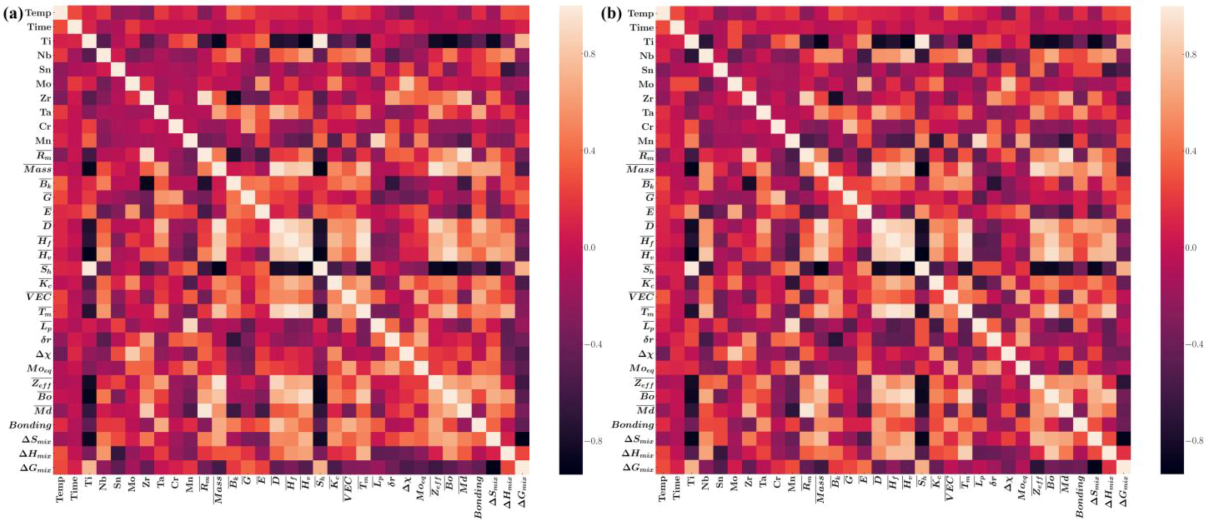
The Pearson product-moment correlation coefficient (PCC) [48] was used to observe the degree of correlation between the features. The p-value was used to measure the degree of correlation between two features. The closer the absolute value was to 1, the stronger the correlation. A positive value indicated a positive correlation and a negative value indicated a negative correlation. From Figure 2a, it can be observed that the absolute values of the p-values between some features are close to 1 in the microstructures dataset. For example, Ti (mass %) was strongly negatively correlated with (the average effective nuclei charges) and (the entropy of mixing), and Ti (mass %) and (specific heat) were strongly positively correlated. Similar results were also obtained from the Young’s modulus dataset, as shown in Figure 2b. Hence, feature selection is required to reduce redundant features. The number of features and the optimal combination of features can be determined.
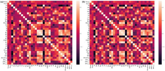
Figure 2.
The heat map describes the correlation between the features of the datasets. The darker the color, the stronger the positive correlation between the features and characteristics; the lighter the color, the stronger the negative correlation: (a) the microstructures dataset and (b) the Young’s modulus dataset.
3.1.2. Forward Sequential Feature Selection
The results are shown in Figure 3. The microstructures and Young’s modulus datasets were processed using the forward sequential feature selection (FSS) method. From Figure 3a, it can be observed that only a few features are initially considered for modeling. It appears that the model is underfitting during the training process due to only a few features supplying a limited amount of information. As the number of features increases, the performance of the model gradually improves and reaches a peak. However, too many features degrade the model’s performance. The reason is that redundant features lead to overfitting. From Figure 3a, it can be observed that the highest prediction accuracy is achieved when the number of features is increased to 7 for the classification model. From Figure 3b, it can be observed that the error reaches a minimum when the number of features is 12 for the regression model. As a result, we finally determined the combination of features with the best cross-validation scores as the features for model training, as shown in Table 2.
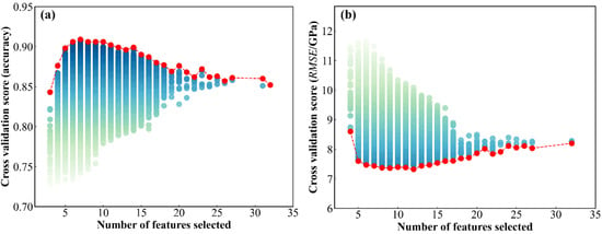
Figure 3.
FSS feature selection results: (a) the microstructures dataset and (b) the Young’s modulus dataset.

Table 2.
The optimal combinations of features were obtained after feature selection, which produces the best performance of the model.
3.2. The Establishment of the Predicting Models
3.2.1. The Predicting Model of the Microstructures
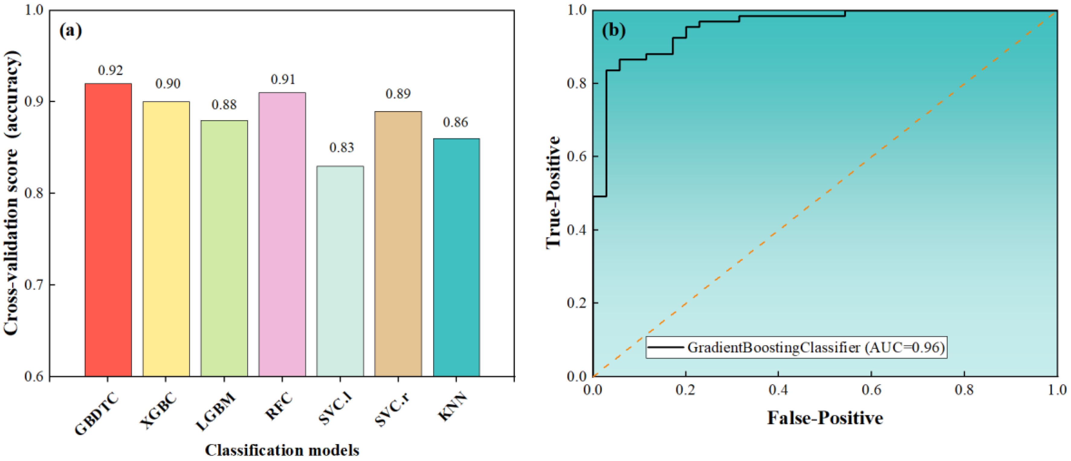
Figure 4a shows the prediction performance of different classification models by five-fold cross validation. Among all the models, the GBDTC model had the highest prediction accuracy with a cross-validation score of 0.92, and the SVC.l and KNN models had the worst prediction accuracies of 0.83 and 0.86 only. Hence, the GBDTC model was used to predict whether it was a β-phase or not.
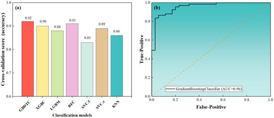
Figure 4.
Evaluation of the classification model’s performances: (a) cross-validation results under different classification models and (b) ROC curve distribution of the GBDTC model on the testing dataset.
After training the GBDTC model on the training dataset, the ROC curve on the testing dataset was obtained, with an AUC value of 0.96, as shown in Figure 4b. It can be concluded that the performance of the GBDTC model for prediction accuracy and generalization ability distinguishes well between β-phase alloys and non-β-phase alloys.
3.2.2. The Predicting Model of Young’s Modulus
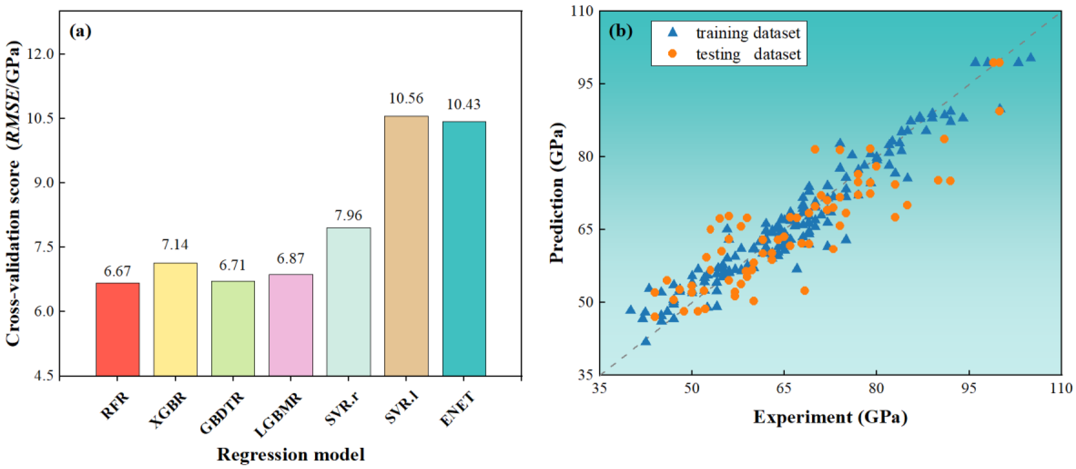
Figure 5a shows the prediction performance of the regression models by five-fold cross validation. The tree-based models had a small cross-validation error, whereas the RFR model had the smallest cross-validation root-mean-square error of 6.67 GPa. The SVR.l and ENET linear models had larger errors because they had difficulty in handling high-dimensional data. In this study, we chose the RFR model to predict the Young’s modulus of the alloys.
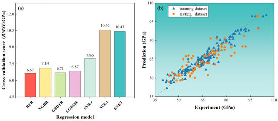
Figure 5.
Evaluation of the regression model’s performances: (a) cross-validation results under different regression models and (b) RFR model prediction on the training dataset and testing dataset.
Figure 5b shows the prediction fits of the RFR model on the training and testing datasets. The blue points are the training dataset, and the RMSE and coefficients on the training set are 2.7 GPa and 0.96, respectively. The orange points are the testing dataset, and the RMSE and coefficients on the testing dataset are 6.21 GPa and 0.78, respectively. It is clear that the data points on both the training and testing datasets are better and that the data points are well distributed in a diagonal shape. The deviation of the predicted values from the experimental values is not significant.
3.3. Feature Importance
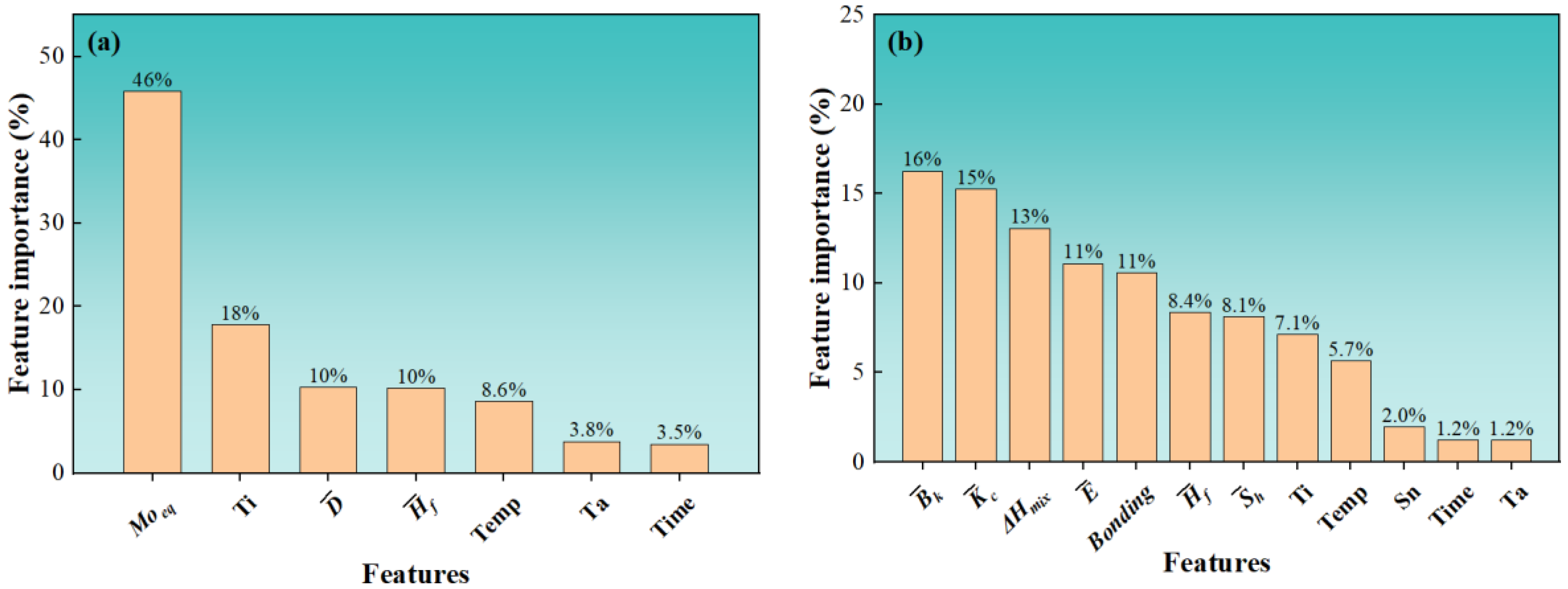
Feature importance is the relative importance score of each feature in making predictions about the model, which is critical for the interpretation of the model. Following the training of the model on the training dataset, the importance of the features was assessed. Figure 6 shows the feature importance calculated by the GBDTC and RFR models, respectively. As shown in Figure 6a, it can be observed that the importance of the feature in the GBDTC model is the highest, at 46%. Additionally, it is much higher than other features and contributes the most to the prediction. From Figure 6b, it can be observed that the features that can be found to influence the RFR model are ; ; ; and Bonding, whose importance is 16%, 15%, 13%, 11%, and 11%, respectively. and are the average bulk modulus and the average Young’s modulus of the alloy, respectively, which are useful for the model to estimate the overall Young’s modulus. Moreover, contributes to the prediction of the model. Since it is a key parameter, it used to describe the stability and phase transformation of the solid solution phase, which, in turn, affects the Young’s modulus of the alloys [49,50,51]. On the other hand, it has been reported that a parameter (Bonding) [41] is proposed to represent the interatomic bonding force of the alloy, which is in good agreement with the Young’s modulus of the alloy. This is in accordance with the predicting results of our models.

Figure 6.
Feature importance analysis, which is used to observe the percentage of importance of features of the predicted target: (a) classification model and (b) regression model.
3.4. Model Validation
3.4.1. Experimental Validation
To validate the prediction accuracy and generalization ability of the models, the compositions of the alloys were chosen in a multi-component system. The predicted chemical composition space of the alloy was Ti–xMo–yNb–zTa–uZr–vSn, where (0 ≤ x, y, z, u, v < 20). With a step size of 1, the predicted compositions had 3200000 possibilities. The Ti–Nb–Ta–Zr system was selected as the master alloy because the system has been extensively studied [52]. The microstructure and Young’s modulus of the alloys of the Ti–Nb–Ta–Zr–Mo/Sn system were predicted.
In the first iteration of the experiments, alloy compositions were randomly selected from the predicted space for experiments, which were predicted to have a single β-phase and the Young’s modulus predicted to be <60 GPa. Two alloys, Ti–19Nb–16Ta–7Zr–4Mo (I-1, wt.%) and Ti–19Nb–5Ta–1Zr–9Sn (I-2, wt.%), were predicted to be single β-phase, and their predicted Young’s moduli were 56.15 GPa and 52.80 GPa, respectively. Then, a series of experimental characterizations and measurements were conducted to verify the predictions.
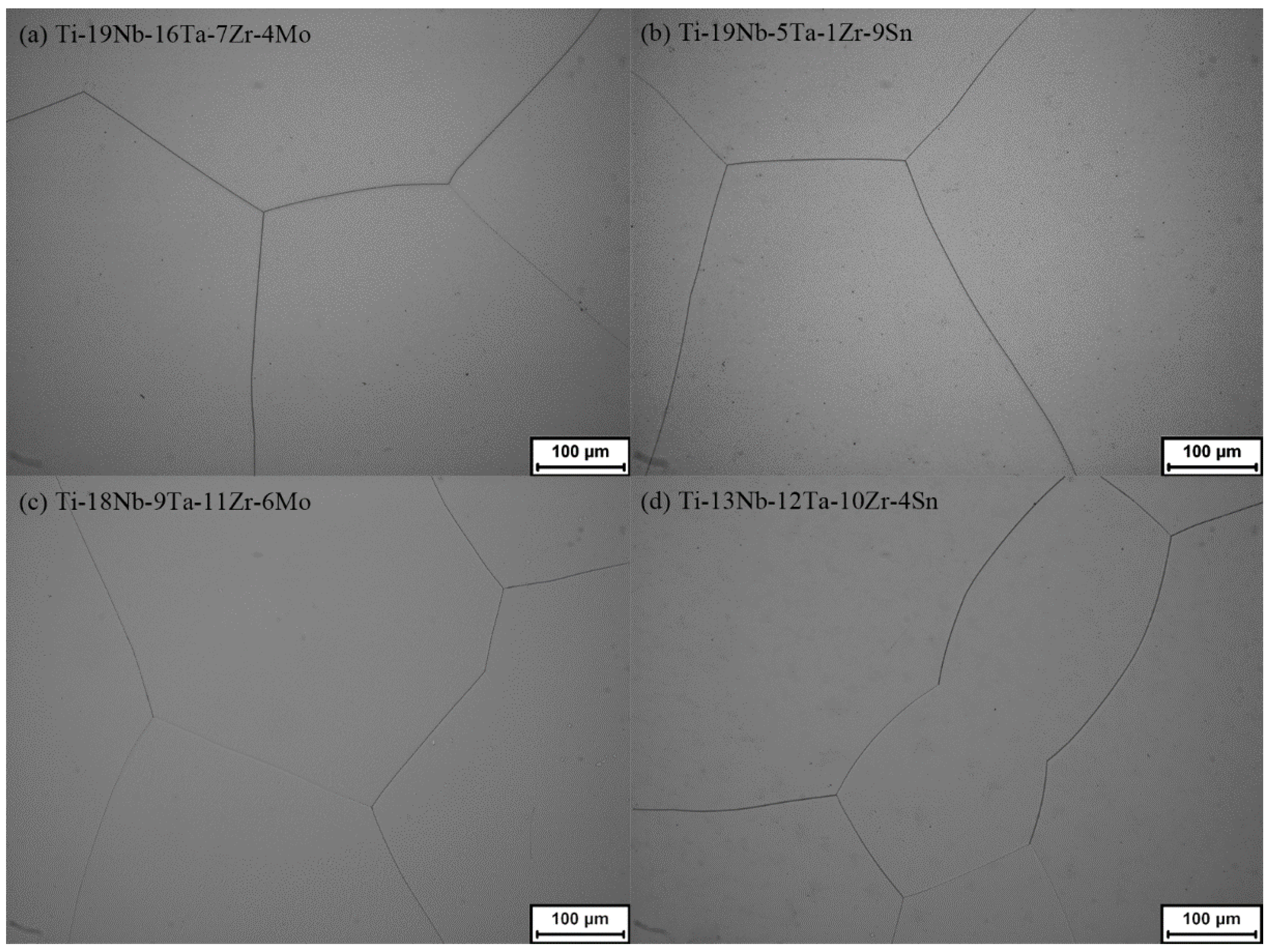
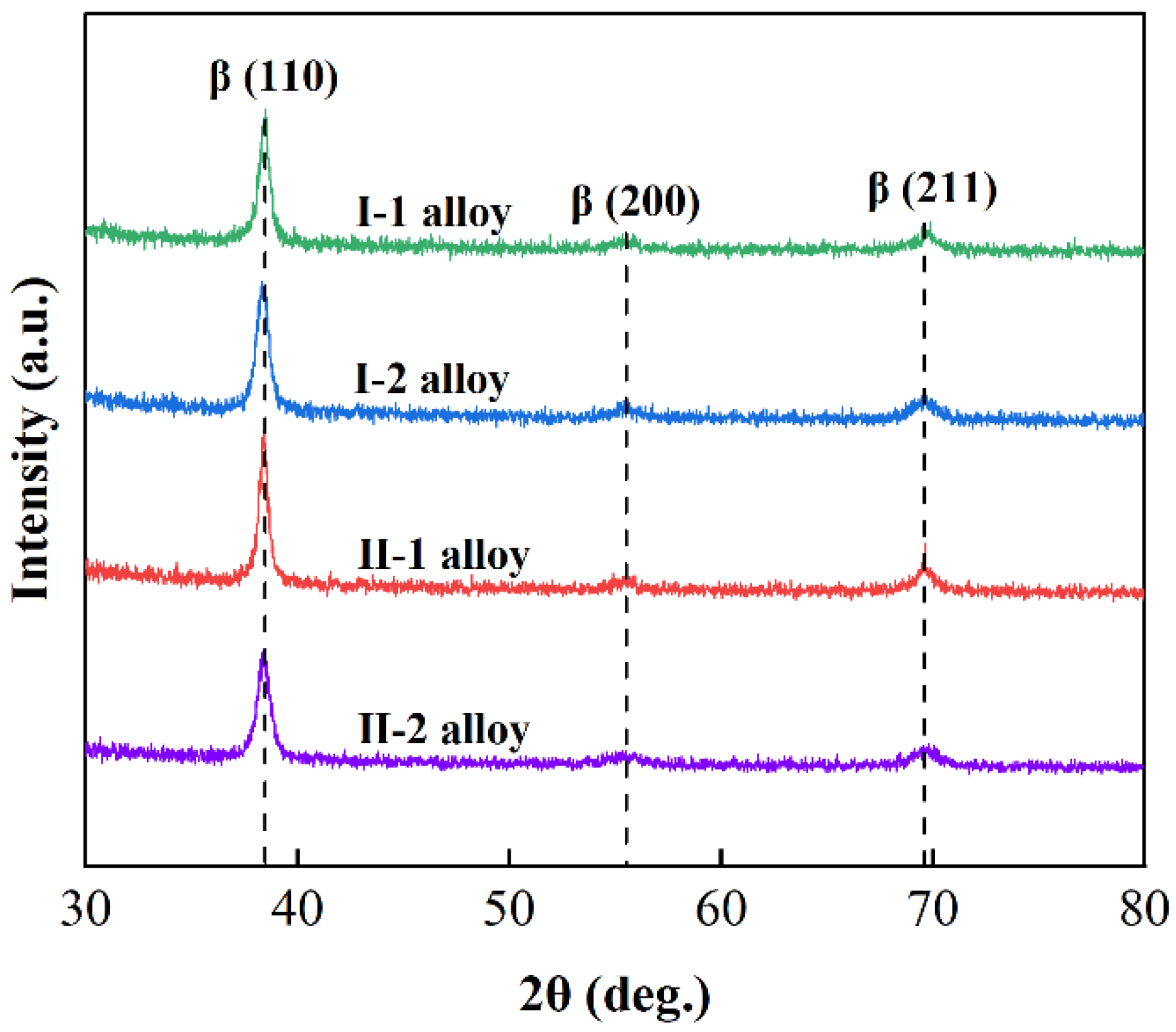
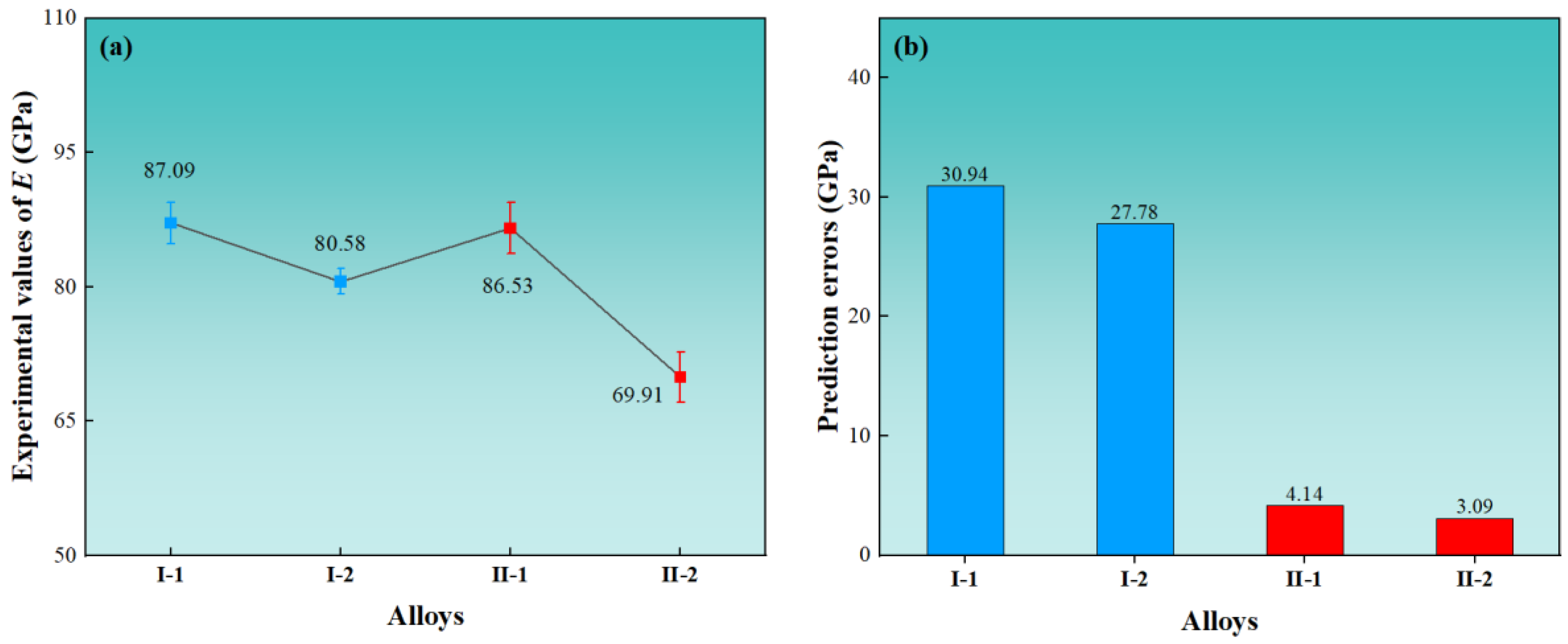
The compositions of the alloys were measured by EDS, see Table 3. As shown in Figure 7, the microstructures of both I-1 and I-2 alloys were the single β-phase observed by optical microscopy. The absence of other phase precipitations was confirmed by the XRD patterns of I-1 and I-2 alloys (Figure 8), where only the β diffraction peaks could be indexed. This is consistent with the predictions of the model. After performing the nanoindentation test, the Young’s modulus of the I-1 and I-2 alloys are shown in Figure 9a. The experimental Young’s modulus values of I-1 and I-2 alloys are 87.09 ± 2.30 GPa and 80.58 ± 1.42 GPa, respectively. Figure 9b shows the errors between the experimentally measured results and the predictions, which are 30.94 GPa and 27.78 GPa, respectively. It can be observed that there is a large difference between them. This is ascribed to the lack of data samples of multi-component β-Ti alloys in the machine learning databases, which could lead to major errors in the model’s predictions. Thus, the experimental data from I-1 and I-2 alloys were fed back to the machine learning databases for training.

Table 3.
The compositions of alloys (wt.%) were measured by EDS and all spectra were recorded at an accelerating voltage of 20 kV.

Figure 7.
Microstructures of the Ti–Mo–Nb–Ta–Zr–Sn alloys were observed by optical microscope after water quenching: (a) Ti–19Nb–16Ta–7Zr–4Mo, (b) Ti–19Nb–5Ta–1Zr–9Sn, (c) Ti–18Nb–9Ta–11Zr–6Mo, and (d) Ti–13Nb–12Ta–10Zr–4Sn.
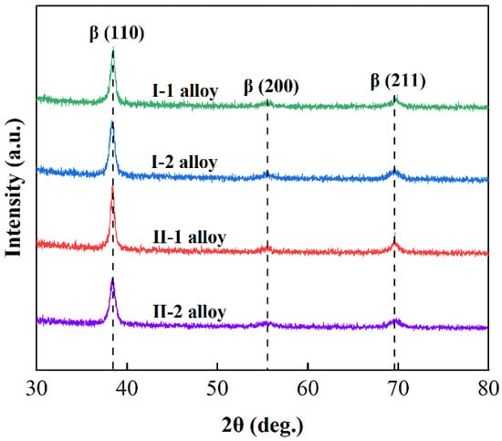
Figure 8.
XRD patterns of the Ti–Mo–Nb–Ta–Zr–Sn alloys.
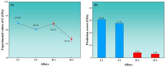
Figure 9.
Comparing experimental and predicted results of Young’s modulus of Ti–Mo–Nb–Ta–Zr–Sn alloys. (a) Young’s modulus of the alloys was measured by the nanoindentation test, and (b) prediction errors of machine learning.
In the second iteration of the experiment, two alloys, Ti–18Nb–9Ta–11Zr–6Mo (II-1, wt.%) and Ti–13Nb–12Ta–10Zr–4Sn (II-2, wt.%), were randomly selected, which were in the same system as the first iteration of the experimental alloys. The II-1 and II-2 alloys were predicted to be single β-phase, and their predicted Young’s moduli were 82.39 GPa and 66.82 GPa, respectively. In Figure 7c,d, it is shown that the microstructures of both II-1 and II-2 alloys are single β-phase. The XRD pattern confirms that alloys II-1 and II-2 only have β-phases. The experimentally measured Young’s moduli for them are 86.53 ± 2.86 GPa and 69.91 ± 2.79 GPa, respectively. The prediction errors of the model are only 4.14 GPa and 3.09 GPa. It can be found that, after the feedback of the experimental data from the previous round, the prediction errors are substantially reduced. The predictions were more accurate and reliable.
3.4.2. Latest Reference Validation
As shown in Table 4, the 9 β-Ti alloy compositions from the latest reported literature were collected to validate the models. These alloys were not included in the machine learning databases. For #1 to #2 alloys, the Young’s modulus increased with the addition of Nb; #3 to #4, Young’s modulus increased with the addition of Mo, which was in agreement with the predictions. For alloys #5 to #9, it is worth noting that the Fe was not included in the machine learning databases. Nevertheless, their Young’s moduli were predicted with an error less than 1.5 GPa. The results show that the models exhibit good robustness and prediction accuracies, providing guiding suggestions for the subsequent optimization of alloy properties.

Table 4.
Alloy compositions and experimental Young’s modulus were collected from the latest reported literature to estimate the prediction performance of the models.
Table 4.
Alloy compositions and experimental Young’s modulus were collected from the latest reported literature to estimate the prediction performance of the models.
| Index | Composition (wt.%) | Experiment E/GPa | Prediction E/GPa | Error E/GPa | Reference |
|---|---|---|---|---|---|
| #1 | Ti–12Nb–12Zr–12Sn | 42 | 47.68 | 5.68 | [53] |
| #2 | Ti–14Nb–12Zr–12Sn | 51 | 48.98 | −2.02 | [53] |
| #3 | Ti–6Nb–3Mo–12Zr–12Sn | 52 | 50.18 | −1.82 | [53] |
| #4 | Ti–6Nb–6Mo–12Zr–12Sn | 69 | 65.15 | −3.85 | [53] |
| #5 | Ti–26Nb–2Fe | 83 | 78.39 | −4.61 | [54] |
| #6 | Ti–26Nb–2Fe–2Sn | 65 | 66.25 | 1.25 | [54] |
| #7 | Ti–26Nb–2Fe–4Sn | 58 | 59.37 | 1.37 | [54] |
| #8 | Ti–26Nb–2Fe–6Sn | 60 | 59.51 | −0.49 | [54] |
| #9 | Ti–26Nb–2Fe–8Sn | 63 | 62.49 | −0.51 | [54] |
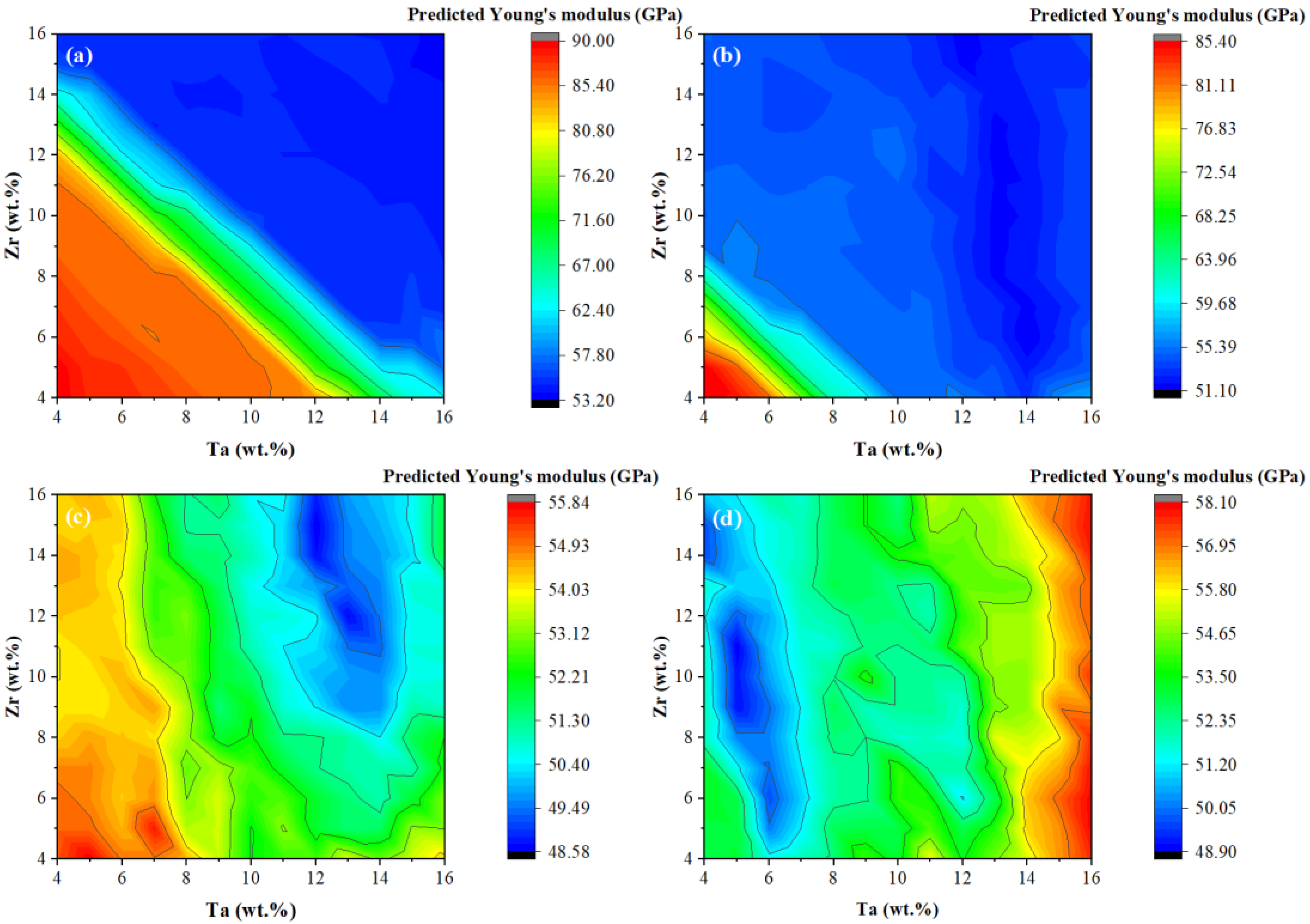
The relationship between Young’s modulus and alloying elements is quite complex, especially for multi-component alloys. In this study, the machine learning model proposed could predict the Young’s modulus in a specific composition space. Its predictions are effective and reliable. However, the prediction model of Young’s modulus is a tree ensemble model, which cannot directly derive a simple function or relation. For the purpose of exploring the dependencies of Young’s modulus on the concentrations of the alloying elements, we predicted Young’s modulus for the alloys of Ti–12Nb–xTa–yZr, Ti–18Nb–xTa–yZr, Ti–24Nb–xTa–yZr and Ti–30Nb–xTa–yZr systems, where 4 < x, y < 16 in steps of 1, as shown in Figure 10. It can be observed in Figure 10a,b that the model predicts a high Young’s modulus when the Nb + Zr + Ta content is less 30 wt.%. The reason was because the precipitation of the hard brittle phase due to the low content of the β stabilizers, which lead to a high Young’s modulus. Some researchers have studied the effects of alloying elements on Young’s modulus in the Ti–Nb–Ta–Zr system. Sakaguchi et al. [55] discovered that the increasing Ta content lead to increasing Young’s modulus in the Ti–30N–XTa–5Zr system when the Ta content increased from 10% to 15%. Additionally, the effect of the Zr element on Young’s modulus was not significant in the Ti–30N–10Ta–XZr system when the Zr content increased from 5% to 10%. Dai et al. [56] found that the Young’s modulus of the Ti–30Nb–5Ta–XZr system decreased when the Zr content increased from 6% to 9%, and the Young’s modulus increased when the Zr content increased from 9% to 15%. Their results are consistent with our predicted results presented in Figure 10d. Additionally, it is worth noting that the lowest predicted Young’s modulus value was 48.58 GPa, presented in Figure 10c. This indicates that the possibility of having a low Young’s modulus in the Ti–Nb–Ta–Zr system, which could provide guidance for the subsequent research work.

Figure 10.
Predicted Young’s modulus of Ti alloy systems by machine learning: (a) Ti–12Nb–xTa–yZr, (b) Ti–18Nb–xTa–yZr, (c) Ti–24Nb–xTa–yZr, and (d) Ti–30Nb–xTa–yZr.
4. Conclusions
In this study, the problems faced by experimental and computational methods for biomedical multicomponent β-Ti alloys were firstly discussed. It was very difficult to test all the possible alloy compositions using traditional methods. Machine learning has become a popular method for designing materials with target properties in the recent years. Due to the limited data collected in materials science, machine learning has some limitations.
Hence, a machine learning prediction method was proposed that could efficiently and reliably predict the microstructures and Young’s moduli of biomedical multi-component β-Ti alloys. The properties affecting the microstructures and Young’s moduli were embedded in the modeling. Firstly, the GBDTC model was the best model to identify the microstructures, and the RFR model was the best model for predicting Young’s modulus. Finally, the experimental results showed that the models had excellent robustness, low prediction errors and the prediction results were in good agreement with the experiments.
With this approach, the Ti–13Nb–12Ta–10Zr–4Sn (wt.%) alloy was prepared with a single β-phase microstructure and a Young’s modulus of 69.91 GPa. The relationship between the composition–microstructure process and parameters–properties of the alloys had good predictive capabilities in the new β systems, which can assist in the design and optimization of novel Ti alloys.
Author Contributions
Conceptualization, X.L., J.Y. and C.W.; Data curation, Q.P., S.P. and J.D.; Formal analysis, Q.P. and S.P.; Investigation, Q.P., Y.L. and J.H.; Methodology, J.H.; Resources, C.W. and X.L.; Software, Q.P.; Supervision, C.W. and X.L.; Visualization, Q.P.; Writing—original draft, Q.P., S.Y. and J.Y.; Writing—review and editing, Q.P. and J.Y. All authors have read and agreed to the published version of the manuscript.
Funding
This research was funded by the Key-area Research and Development Program of Guang Dong Province (Grant No. 2019B010943001), the Major-Special Science and Technology Project in Shandong Province (Grant No. 2019JZZY010303), and the National Post-doctoral Program for Innovative Talents (Grant No. BX20200103).
Institutional Review Board Statement
Not applicable.
Informed Consent Statement
Not applicable.
Data Availability Statement
The data presented in this study are available on request from the corresponding author. The data are not publicly available due to its privacy.
Conflicts of Interest
The authors declare no competing interests.
References
- Niinomi, M.; Liu, Y.; Nakai, M.; Liu, H.; Li, H. Biomedical titanium alloys with Young’s moduli close to that of cortical bone. Regen. Biomater. 2016, 3, 173–185. [Google Scholar] [CrossRef] [PubMed]
- Wang, Q.; Dong, C.; Liaw, P.K. Structural Stabilities of β-Ti Alloys Studied Using a New Mo Equivalent Derived from [β/(α + β)] Phase-Boundary Slopes. Metall. Mater. Trans. A 2015, 46, 3440–3447. [Google Scholar] [CrossRef]
- Sumitomo, N.; Noritake, K.; Hattori, T.; Morikawa, K.; Niwa, S.; Sato, K.; Niinomi, M. Experiment study on fracture fixation with low rigidity titanium alloy. J. Mater. Sci. Mater. Med. 2008, 19, 1581–1586. [Google Scholar] [CrossRef] [PubMed]
- Abdel-Hady Gepreel, M.; Niinomi, M. Biocompatibility of Ti-alloys for long-term implantation. J. Mech. Behav. Biomed. Mater. 2013, 20, 407–415. [Google Scholar] [CrossRef] [PubMed]
- Eisenbarth, E.; Velten, D.; Müller, M.; Thull, R.; Breme, J. Biocompatibility of β-stabilizing elements of titanium alloys. Biomaterials 2004, 25, 5705–5713. [Google Scholar] [CrossRef] [PubMed]
- Long, M.; Rack, H.J. Titanium alloys in total joint replacement—A materials science perspective. Biomaterials 1998, 19, 1621–1639. [Google Scholar] [CrossRef]
- Niinomi, M. Mechanical properties of biomedical titanium alloys. Mater. Sci. Eng. A 1998, 243, 231–236. [Google Scholar] [CrossRef]
- Sidhu, S.S.; Singh, H.; Gepreel, M.A.-H. A review on alloy design, biological response, and strengthening of β-titanium alloys as biomaterials. Mater. Sci. Eng. C 2021, 121, 111661. [Google Scholar] [CrossRef]
- Li, P.; Ma, X.; Tong, T.; Wang, Y. Microstructural and mechanical properties of β-type Ti–Mo–Nb biomedical alloys with low elastic modulus. J. Alloys Compd. 2020, 815, 152412. [Google Scholar] [CrossRef]
- Wang, P.; Wu, L.; Feng, Y.; Bai, J.; Zhang, B.; Song, J.; Guan, S. Microstructure and mechanical properties of a newly developed low Young’s modulus Ti–15Zr–5Cr–2Al biomedical alloy. Mater. Sci. Eng. C 2017, 72, 536–542. [Google Scholar] [CrossRef]
- Zhao, Z.; Lee, K. Effect of Alloying Elements on Plastic Workability and Corrosion Behavior of Ti-X (X = 6 Co, 8 Cr, 4 Fe, 6 Mn, 10 Mo, and 36 Nb) Binary Alloys. Arch. Met. Mater. 2017, 62, 1185–1190. [Google Scholar] [CrossRef][Green Version]
- Mehjabeen, A.; Xu, W.; Qiu, D.; Qian, M. Redefining the β-Phase Stability in Ti-Nb-Zr Alloys for Alloy Design and Microstructural Prediction. JOM 2018, 70, 2254–2259. [Google Scholar] [CrossRef]
- Zhao, X.; Niinomi, M.; Nakai, M.; Miyamoto, G.; Furuhara, T. Microstructures and mechanical properties of metastable Ti–30Zr–(Cr, Mo) alloys with changeable Young’s modulus for spinal fixation applications. Acta Biomater. 2011, 7, 3230–3236. [Google Scholar] [CrossRef] [PubMed]
- Liang, S.; Feng, X.; Yin, L.; Liu, X.; Ma, M.; Liu, R. Development of a new β Ti alloy with low modulus and favorable plasticity for implant material. Mater. Sci. Eng. C 2016, 61, 338–343. [Google Scholar] [CrossRef]
- Li, Y.; Yang, C.; Wang, F.; Zhao, H.; Qu, S.; Li, X.; Zhang, W. Biomedical TiNbZrTaSi alloys designed by d-electron alloy design theory. Mater. Des. 2015, 85, 7–13. [Google Scholar] [CrossRef]
- Chen, W.; Li, W.; Du, Y. Investigations on diffusion behaviors in Ti–rich Ti–Nb–Zr–Cr system: Experimental measurement and CALPHAD modeling. Calphad 2018, 62, 223–231. [Google Scholar] [CrossRef]
- Tan, J.; Xu, G.; Tao, X.; Chen, F.; Cui, Y.; Zhou, L. CALPHAD assessment of bio-oriented Ti–Zr–Sn system and experimental validation in Ti/Zr-rich alloys. Calphad 2019, 67, 101686. [Google Scholar] [CrossRef]
- Song, Y.; Xu, D.; Yang, R.; Li, D.; Wu, W.; Guo, Z.X. Theoretical study of the effects of alloying elements on the strength and modulus of β-type bio-titanium alloys. Mater. Sci. Eng. A 1999, 260, 269–274. [Google Scholar] [CrossRef]
- Raabe, D.; Sander, B.; Friák, M.; Ma, D.; Neugebauer, J. Theory-guided bottom-up design of β-titanium alloys as biomaterials based on first principles calculations: Theory and experiments. Acta Mater. 2007, 55, 4475–4487. [Google Scholar] [CrossRef]
- Luo, M.; Liang, L.; Lang, L.; Xiao, S.; Hu, W.; Deng, H. Molecular dynamics simulations of the characteristics of Mo/Ti interfaces. Comput. Mater. Sci. 2018, 141, 293–301. [Google Scholar] [CrossRef]
- Song, J.; Wang, L.; Zhang, L.; Wu, W.; Gao, Z. First-principles molecular dynamics studying the solidification of Ti-6Al-4V alloy. J. Mol. Liq. 2020, 315, 113606. [Google Scholar] [CrossRef]
- Vivanco-Benavides, L.E.; Martínez-González, C.L.; Mercado-Zúñiga, C.; Torres-Torres, C. Machine learning and materials informatics approaches in the analysis of physical properties of carbon nanotubes: A review. Comput. Mater. Sci. 2022, 201, 110939. [Google Scholar] [CrossRef]
- Juan, Y.; Dai, Y.; Yang, Y.; Zhang, J. Accelerating materials discovery using machine learning. J. Mater. Sci. Technol. 2021, 79, 78–190. [Google Scholar] [CrossRef]
- Liu, Y.; Esan, O.C.; Pan, Z.; An, L. Machine learning for advanced energy materials. Energy AI 2021, 3, 100049. [Google Scholar] [CrossRef]
- Yu, J.; Xi, S.; Pan, S.; Wang, Y.; Peng, Q.; Shi, R.; Wang, C.; Liu, X. Machine learning-guided design and development of metallic structural materials. J. Mater. Inform. 2021, 1, 9. [Google Scholar] [CrossRef]
- Pan, S.; Wang, Y.; Yu, J.; Yang, M.; Zhang, Y.; Wei, H.; Chen, Y.; Wu, J.; Han, J.; Wang, C.; et al. Accelerated discovery of high-performance Cu-Ni-Co-Si alloys through machine learning. Mater. Des. 2021, 209, 109929. [Google Scholar] [CrossRef]
- Yu, J.; Guo, S.; Chen, Y.; Han, J.; Lu, Y.; Jiang, Q.; Wang, C.; Liu, X. A two-stage predicting model for γ′ solvus temperature of L12-strengthened Co-base superalloys based on machine learning. Intermetallics 2019, 110, 106466. [Google Scholar] [CrossRef]
- Yu, J.; Wang, C.; Chen, Y.; Wang, C.; Liu, X. Accelerated design of L12-strengthened Co-base superalloys based on machine learning of experimental data. Mater. Des. 2020, 195, 108996. [Google Scholar] [CrossRef]
- Honysz, R. Modeling the Chemical Composition of Ferritic Stainless Steels with the Use of Artificial Neural Networks. Metals 2021, 11, 724. [Google Scholar] [CrossRef]
- Churyumov, A.; Kazakova, A.; Churyumova, T. Modelling of the Steel High-Temperature Deformation Behaviour Using Artificial Neural Network. Metals 2022, 12, 447. [Google Scholar] [CrossRef]
- Yang, F.; Li, Z.; Wang, Q.; Jiang, B.; Yan, B.; Zhang, P.; Xu, W.; Dong, C.; Liaw, P.K. Cluster-formula-embedded machine learning for design of multicomponent β-Ti alloys with low Young’s modulus. npj Comput. Mater. 2020, 6, 101. [Google Scholar] [CrossRef]
- Wu, C.-T.; Chang, H.-T.; Wu, C.-Y.; Chen, S.-W.; Huang, S.-Y.; Huang, M.; Pan, Y.-T.; Bradbury, P.; Chou, J.; Yen, H.-W. Machine learning recommends affordable new Ti alloy with bone-like modulus. Mater. Today 2019, 34, 41–50. [Google Scholar] [CrossRef]
- Xiong, S.; Li, X.; Wu, X.; Yu, J.; Gorbatov, O.I.; Di Marco, I.; Kent, P.R.; Sun, W. A combined machine learning and density functional theory study of binary Ti-Nb and Ti-Zr alloys: Stability and Young’s modulus. Comput. Mater. Sci. 2020, 184, 109830. [Google Scholar] [CrossRef]
- Zhang, H.; Fu, H.; Zhu, S.; Yong, W.; Xie, J. Machine learning assisted composition effective design for precipitation strengthened copper alloys. Acta Mater. 2021, 215, 117118. [Google Scholar] [CrossRef]
- Yuan, R.; Xue, D.; Xue, D.; Li, J.; Ding, X.; Sun, J.; Lookman, T. Knowledge-Based Descriptor for the Compositional Dependence of the Phase Transition in BaTiO3-Based Ferroelectrics. ACS Appl. Mater. Interfaces 2020, 12, 44970–44980. [Google Scholar] [CrossRef]
- Zhang, Y.; Wen, C.; Wang, C.; Antonov, S.; Xue, D.; Bai, Y.; Su, Y. Phase prediction in high entropy alloys with a rational selection of materials descriptors and machine learning models. Acta Mater. 2019, 185, 528–539. [Google Scholar] [CrossRef]
- Xiong, J.; Shi, S.-Q.; Zhang, T.-Y. A machine-learning approach to predicting and understanding the properties of amorphous metallic alloys. Mater. Des. 2020, 187, 108378. [Google Scholar] [CrossRef]
- W.R. Inc. Properties of the Elements. 2021. Available online: https://periodictable.com/Properties/ (accessed on 1 August 2020).
- Guo, S.; Ng, C.; Lu, J.; Liu, C.T. Effect of valence electron concentration on stability of fcc or bcc phase in high entropy alloys. J. Appl. Phys. 2011, 109, 103505. [Google Scholar] [CrossRef]
- Jiang, B.; Wang, Q.; Wen, D.; Xu, F.; Chen, G.; Dong, C.; Sun, L.; Liaw, P.K. Effects of Nb and Zr on structural stabilities of Ti-Mo-Sn-based alloys with low modulus. Mater. Sci. Eng. A 2017, 687, 1–7. [Google Scholar] [CrossRef]
- You, L.; Song, X. A study of low Young′s modulus Ti–Nb–Zr alloys using d electrons alloy theory. Scr. Mater 2012, 67, 57–60. [Google Scholar] [CrossRef]
- Khaire, U.M.; Dhanalakshmi, R. Stability of feature selection algorithm: A review. J. King Saud Univ. Comput. Inf. Sci. 2019, 34, 1060–1073. [Google Scholar] [CrossRef]
- Bengio, Y.; Grandvalet, Y. Bias in Estimating the Variance of K-Fold Cross-Validation. In Statistical Modeling and Analysis for Complex Data Problems; Duchesne, P., RÉMillard, B., Eds.; Springer: Boston, MA, USA, 2005; pp. 75–95. [Google Scholar]
- Pedregosa, F.; Varoquaux, G.; Gramfort, A.; Michel, V.; Thirion, B.; Grisel, O.; Blondel, M.; Prettenhofer, P.; Weiss, R.; Dubourg, V.; et al. Scikit-learn: Machine learning in Python. J. Mach. Learn. Res. 2011, 12, 2825–2830. [Google Scholar]
- Chen, T.; Guestrin, C. XGBoost: A Scalable Tree Boosting System. In Proceedings of the 22nd ACM SIGKDD International Conference on Knowledge Discovery and Data Mining, Association for Computing Machinery, San Francisco, CA, USA, 13–17 August 2016; pp. 785–794. [Google Scholar]
- Ke, G.; Meng, Q.; Finley, T.; Wang, T.; Chen, W.; Ma, W.; Ye, Q.; Liu, T.Y. Lightgbm: A highly efficient gradient boosting decision tree. Adv. Neural Inf. Process. Syst. 2017, 30, 3146–3154. [Google Scholar]
- Bergstra, J.; Yamins, D.; Cox, D.D. Hyperopt: A Python Library for Optimizing the Hyperparameters of Machine Learning Algorithms. In Proceedings of the 12th Python in Science Conference, Austin, TX, USA, 24–29 June 2013; p. 20. [Google Scholar]
- Puth, M.-T.; Neuhäuser, M.; Ruxton, G.D. Effective use of Pearson’s product–moment correlation coefficient. Anim. Behav. 2014, 93, 183–189. [Google Scholar] [CrossRef]
- Guo, S.; Liu, C.T. Phase stability in high entropy alloys: Formation of solid-solution phase or amorphous phase. Prog. Nat. Sci. Mater. Int. 2011, 21, 433–446. [Google Scholar] [CrossRef]
- Xu, X.; Guo, S.; Nieh, T.; Liu, C.; Hirata, A.; Chen, M. Effects of mixing enthalpy and cooling rate on phase formation of AlxCoCrCuFeNi high-entropy alloys. Materialia 2019, 6, 100292. [Google Scholar] [CrossRef]
- Roy, A.; Babuska, T.; Krick, B.; Balasubramanian, G. Machine learned feature identification for predicting phase and Young’s modulus of low-, medium- and high-entropy alloys. Scr. Mater 2020, 185, 152–158. [Google Scholar] [CrossRef]
- Niinomi, M.; Nakai, M.; Hieda, J. Development of new metallic alloys for biomedical applications. Acta Biomater. 2012, 8, 3888–3903. [Google Scholar] [CrossRef]
- Wu, C.-T.; Lin, P.-H.; Huang, S.-Y.; Tseng, Y.-J.; Chang, H.-T.; Li, S.-Y.; Yen, H.-W. Revisiting alloy design of low-modulus biomedical β-Ti alloys using an artificial neural network. Materialia 2022, 21, 101313. [Google Scholar] [CrossRef]
- Li, Q.; Liu, T.; Li, J.; Cheng, C.; Niinomi, M.; Yamanaka, K.; Chiba, A.; Nakano, T. Microstructure, mechanical properties, and cytotoxicity of low Young’s modulus Ti–Nb–Fe–Sn alloys. J. Mater. Sci. 2022, 57, 5634–5644. [Google Scholar] [CrossRef]
- Sakaguchi, N.; Mitsuo, N.; Akahori, T.; Saito, T.; Furuta, T. Effects of Alloying Elements on Elastic Modulus of Ti-Nb-Ta-Zr System Alloy for Biomedical Applications. Mater. Sci. Forum 2004, 449-452, 1269–1272. [Google Scholar] [CrossRef]
- Dai, S.-J.; Wang, Y.; Chen, F.; Yu, X.-Q.; Zhang, Y.-F. Design of new biomedical titanium alloy based on d-electron alloy design theory and JMatPro software. Trans. Nonferrous Met. Soc. China 2013, 23, 3027–3032. [Google Scholar] [CrossRef]
Publisher’s Note: MDPI stays neutral with regard to jurisdictional claims in published maps and institutional affiliations. |
© 2022 by the authors. Licensee MDPI, Basel, Switzerland. This article is an open access article distributed under the terms and conditions of the Creative Commons Attribution (CC BY) license (https://creativecommons.org/licenses/by/4.0/).

