In Situ X-ray Radiography and Computational Modeling to Predict Grain Morphology in β-Titanium during Simulated Additive Manufacturing

Abstract

The continued development of metal additive manufacturing (AM) has expanded the engineering metallic alloys for which these processes may be applied, including beta-titanium alloys with desirable strength-to-density ratios. To understand the response of beta-titanium alloys to AM processing, solidification and microstructure evolution needs to be investigated. In particular, thermal gradients (Gs) and solidification velocities (Vs) experienced during AM are needed to link processing to microstructure development, including the columnar-to-equiaxed transition (CET). In this work, in situ synchrotron X-ray radiography of the beta-titanium alloy Ti-10V-2Fe-3Al (wt.%) (Ti-1023) during simulated laser-powder bed fusion (L-PBF) was performed at the Advanced Photon Source at Argonne National Laboratory, allowing for direct determination of Vs. Two different computational modeling tools, SYSWELD and FLOW-3D, were utilized to investigate the solidification conditions of spot and raster melt scenarios. The predicted Vs obtained from both pieces of computational software exhibited good agreement with those obtained from in situ synchrotron X-ray radiography measurements. The model that accounted for fluid flow also showed the ability to predict trends unobservable in the in situ synchrotron X-ray radiography, but are known to occur during rapid solidification. A CET model for Ti-1023 was also developed using the Kurz–Giovanola–Trivedi model, which allowed modeled Gs and Vs to be compared in the context of predicted grain morphologies. Both pieces of software were in agreement for morphology predictions of spot-melts, but drastically differed for raster predictions. The discrepancy is attributable to the difference in accounting for fluid flow, resulting in magnitude-different values of Gs for similar Vs.

1. Introduction

The continued development of metal additive manufacturing (AM) over the past couple of decades has expanded the applications and material classes in which these processes can be used. Titanium (Ti) alloys have been at the center of this development, due to their superior properties, particularly for aerospace and defense applications. Although Ti-6Al-4V (Ti-64) has typically dominated in terms of use and research pertaining to metal AM processes, metastable β-Ti alloys have begun to find increased use over Ti-64 (an α + β alloy), due to their increased strength-to-density ratios, among other properties [1]. These metastable β-Ti alloys differ from other classifications of Ti in that the high-temperature β-phase may be retained upon quenching to room temperature, which is of relevance to AM processes [2,3]. The ability to maintain this metastable β-phase is a result of sufficient additions of β-phase stabilizing elements, such as vanadium (V) or molybdenum (Mo). Although sufficient amounts of β-phase stabilizing elements can be added to create stable β-Ti alloys, where the β-phase is retained even at slow cooling rates, they are of more limited use for engineering applications. Throughout the rest of this paper, metastable β-Ti alloys will be referred to as simply β-Ti alloys.

AM technology has allowed for an increased amount of applications in which AM can add value, however many metal-AM processes create parts with anisotropy. This is primarily due to the large columnar grains that can grow along the build height. For this reason, there has been a desire to develop ways to break up these grains to produce ones that are more equiaxed and much smaller in size. These equiaxed grains yield more isotropic mechanical properties that are typically more favorable for structural applications. Approaches such as melt-pool manipulation, modification of alloy composition, and alteration of processing parameters have proven to be successful in increasing regions of equiaxed grains [4,5,6,7]. Of the aforementioned techniques, parameter alteration has been the dominant research focus, because it does not add any significant cost or complexity to the process that other approaches might. This has led to widespread investigation of microstructure–processing links in AM alloys [8,9,10]. For Ti-alloys, this has primarily been conducted for Ti-64 [11,12,13,14,15], where a thorough understanding of the microstructure–processing link has allowed for the use of AM-produced Ti-64 parts in aircraft [16]. Meanwhile, work in the realm of β-Ti alloys has been mostly limited to the “printability” of the material and resulting mechanical properties [17,18].

In order to advance this alloy field for AM, correlations between microstructures and processing parameters, similar to those for Ti-64, are needed. This allows not only for an increased chance of a successful build, but also for the ability to create site-specific microstructures and properties within a single part [19,20], an impossibility with other manufacturing processes. To do this, an alloy-specific solidification map and an understanding of where scan strategies typically fall within this map are needed. A solidification map relates thermal gradients (Gs) and solid–liquid interface velocities (Vs) during solidification to resultant grain morphologies. These predicted maps are typically available in the literature for ubiquitous engineering alloys, but not for β-Ti alloys. Kobyrn et al. used Hunt-criterion boundary lines to classify columnar, mixed, or equiaxed regions based on experimental observations of grain morphologies in Ti-64 for a variety of processes [21]. Their solidification map has widely been accepted and used to predict grain morphologies in AM of Ti-64 [15,22,23]. To create a map for β-Ti alloys using a similar technique, knowledge of resulting Gs and Vs is required. The small size of L-PBF melt pools makes it difficult to obtain accurate Vs using commercial data-collection equipment. For this reason, high-spatial-resolution experiments at national user facilities can be used to determine Vs under L-PBF conditions [24]. Local Gs, on the other hand, are impossible to obtain using almost any experimental setup. For this reason, simulation tools are typically required to predict Gs at all points on the solid–liquid interface [25]. The combinations of Gs and Vs, coupled with an alloy-specific solidification map, then provide the necessary information needed to draw conclusions on the effect of processing parameters on as-built microstructures.

In this study, in situ synchrotron X-ray radiography of simulated L-PBF of the β-Ti alloy Ti-10V-2Fe-3Al (wt.%) (Ti-1023) was used to determine solidification velocities as a function of time and location within the melt pool. Conduction of these experiments at the Advanced Photon Source (APS) at Argonne National Laboratory (ANL) provided the desired spatial and temporal resolutions needed to quantify solidification velocities as a function of position and time within the micron-sized melt-pools characteristic of L-PBF. The corresponding widths and depths of the melt pools were used to calibrate models from two pieces of computational software, SYSWELD and FLOW-3D. The predicted Vs from these tools were compared to those obtained from the in situ synchrotron X-ray radiography to assess the ability of each software to model the complexity of solidification events occurring within the simulated L-PBF melt pools. Additionally, the combinations of Gs and Vs from the models were compared to each other in the context of predicted grain morphologies from a developed CET model for Ti-1023.

2. Experimental Setup

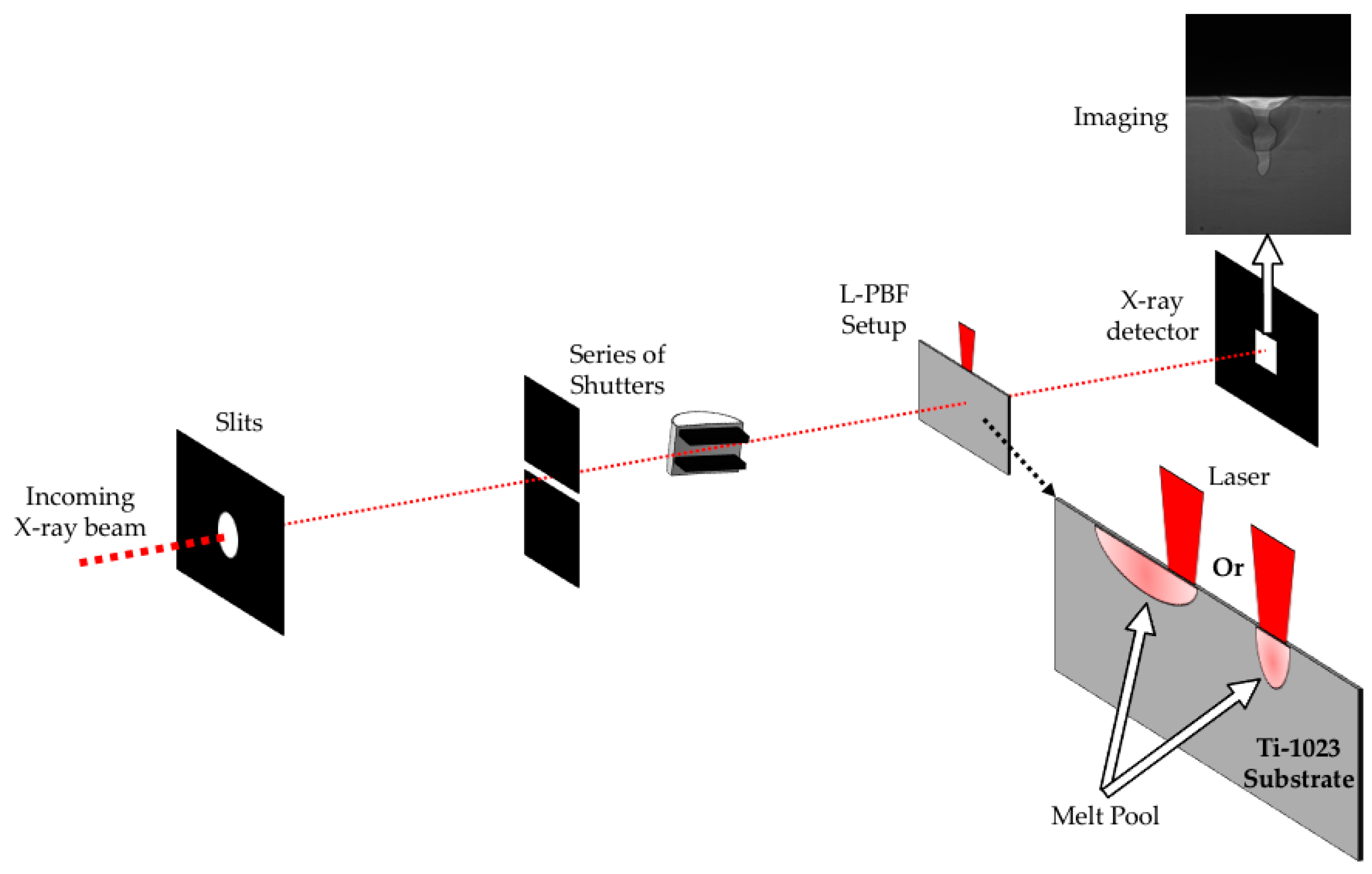
2.1. APS L-PBF Simulator and In Situ X-ray Radiography

In order to obtain Vs at locations along the melt-pool, laser powder bed fusion (L-PBF) simulator experiments were performed at the Sector 32-ID-B beamline at the Advanced Photon Source (APS) at Argonne National Laboratory (ANL), similar to those conducted by Zhao et al. [24]. A schematic of the experimental setup is shown below in Figure 1. Images of the experiments were collected using 80,000 frames/s. In order to purely study the rapid solidification of the alloy under L-PBF conditions, approximately 200 μm thick Ti-1023 substrates were used, instead of powder. Spot-melts were performed using powers of 82 W, 139 W, and 197 W and constant 1 ms dwell times, while 1.5 mm length rasters were completed at powers ranging from 54 W to 512 W and travel speeds of 0.25–2.00 m/s. A wide set of parameters were selected to achieve a variety of solidification conditions and grain morphologies within the samples. Additionally, all experiments were conducted at room temperature and in an inert atmosphere of argon gas.

The resulting imaging of each experiment was used to determine the observed solid–liquid interface velocity as a function of position in the melt pool. This was done using an ImageJ macro, where the solid–liquid interface was identified through a manual selection of points for each frame. Data were then compiled and converted into a set of points that described the evolution of the melt pool as a function of time. A Python script was then utilized to fit a polynomial to each melt pool and to calculate the change in position as a function of time for a specified direction of interest, i.e., across the top of the melt pool, or from the bottom to the top of the melt pool. The in situ radiography was also used to provide maximum depth measurements of the melt pools, while postmortem, top-down secondary electron imaging (SEI) using a Tescan S8252G scanning electron microscope provided the maximum widths, which together, helped to calibrate the final simulations in the modeling work.

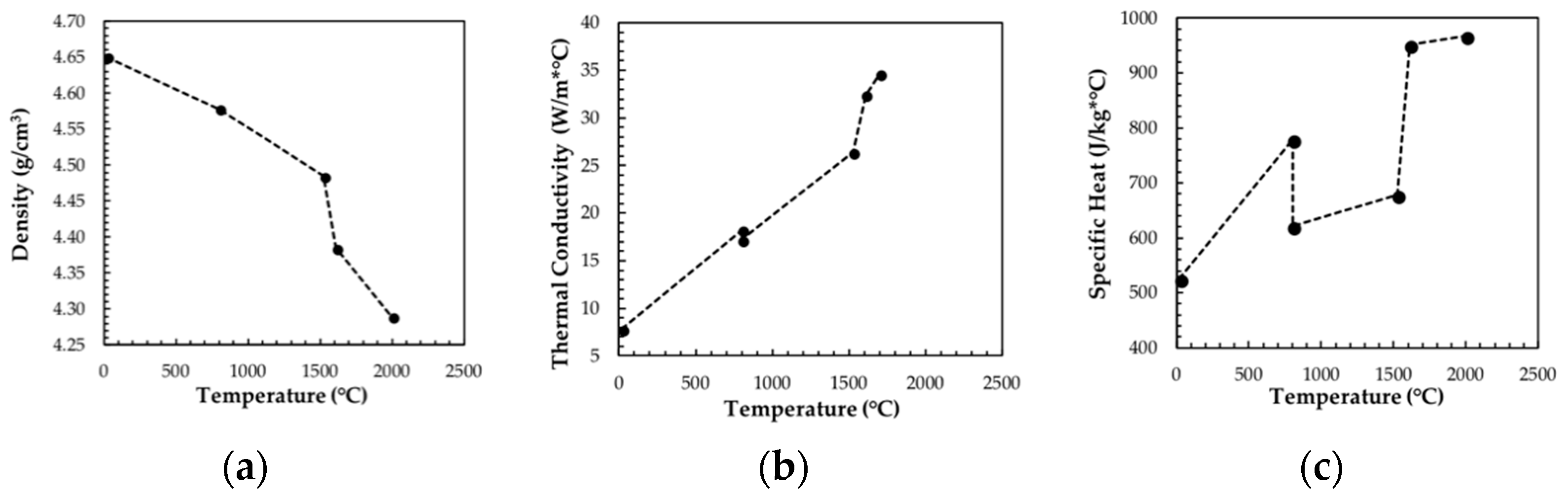
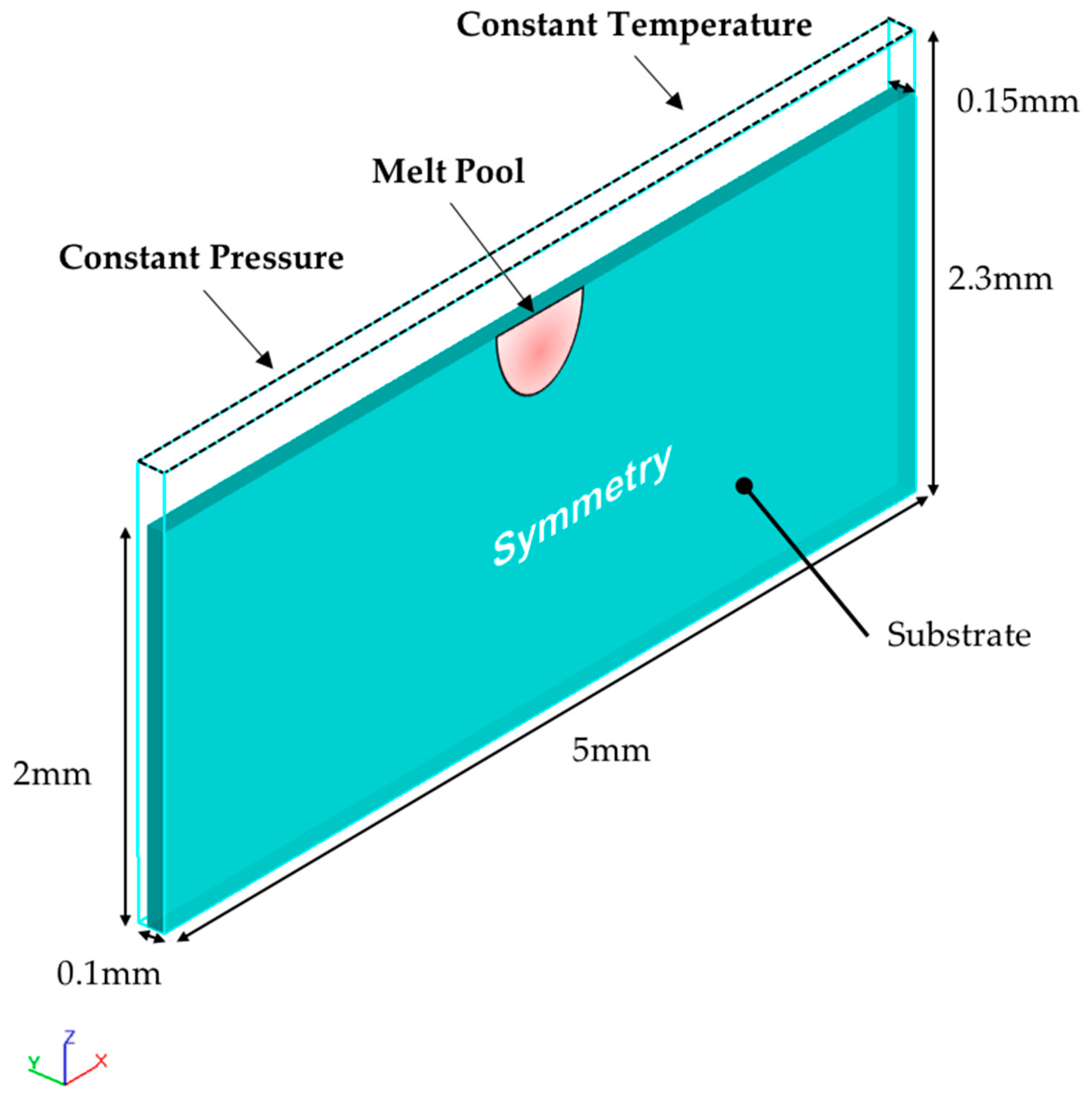
2.2. Model Setup and Inputs

Initial modeling of the APS experiments described above was conducted using a conduction-only commercial software tool called SYSWELD. Although SYSWELD is intended for fusion welding applications, the APS experiments resembled simple laser welding and were assumed to fit within the capabilities of the software. To begin the modeling of these experiments, thermophysical material properties of Ti-1023 were needed. The testing and development of material property databases are notoriously lacking and only exist for a select number of engineering alloys. For Ti, these properties are only widely available for pure Ti and Ti-64 [26]. Due to Ti-64 being an α + β alloy and Ti-1023 being a β alloy, Ti-64 properties were not used as approximations for Ti-1023. With no extensive research on the thermophysical properties of β-Ti, thermodynamic prediction software was used to predict these properties for Ti-1023 whenever possible. Density and specific heat as a function of temperature were obtained using Thermo-Calc TCTI/Ti-alloys database version 3 [27]. Although the database was not robust enough to directly calculate these values, simple relationships were used. For instance, enthalpy is a direct output of the software, but to obtain specific heat, the derivative of enthalpy with respect to temperature was taken to approximate specific heat. Thermal conductivity is another important property; however, the Ti database used in this work was not mature enough to predict this quantity. Taking into account the approximate beta-transition temperature predicted by Thermo-Calc, the thermal conductivity as a function of temperature for Ti-64 from Mills [26] was modified to reflect an approximate set of values for Ti-1023. These estimated thermophysical properties were used as material property input for the following models and are shown in Figure 2.

The specific geometry used within SYSWELD to simulate the various experimental spot-melt and raster conditions is presented in Figure 3. In the melt region of the model, the mesh size was 10 μm × 10 μm × 10 μm and progressively coarsened to decrease the computational time of the simulation. The size of this mesh was limited by the capabilities of SYSWELD, due to problems encountered performing simulations with smaller mesh sizes. The specific experiments simulated within SYSWELD are presented in

Table 1. Process parameters of the modeled spot-melt and raster experiments.

Experiment	Power (W)	Travel Speed (m/s) or Dwell Time (ms)	Energy Input (J/m)
Spot-melt	82	1	-
Spot-melt	139	1	-
Spot-melt	197	1	-
Raster	53.5	0.25	214
Raster	82	0.50	164
Raster	139	0.50	278

. For each condition, the simulation needed to be calibrated using an iterative process of manipulating the dimensions of the Gaussian heat source and efficiency term, until the simulated melt pool dimensions agreed with those obtained from experiments. Additionally, the initial temperature of the substrate for these models was 293 K.

Another commercial software tool, FLOW-3D, was used to simulate the same L-PBF conditions modeled within SYSWELD. FLOW-3D is a computational fluid dynamics (CFD) software and is significantly more computationally intensive than SYSWELD. It accounts for more complicated melt pool dynamics, such as evaporation, surface tension, and convective heat transfer. As a result of this complexity, additional material properties were required to fully capture the complexity of the melt pools. Similar to the reasons discussed above for density, thermal conductivity, and specific heat, many of these properties are not readily available for Ti-1023. In addition, current thermodynamic calculation software is unable to predict them, as was performed for density and specific heat. For this reason, values reported for Ti-64 were used when necessary. All the relevant material properties are listed in

Table 2. Material property inputs for FLOW-3D.

Property	Value	Reference
Surface Tension Coefficient	1.5 N/m	[28]
Surface Tension Temperature Dependence	−2.6 × 10−4 N/m/K
Solidus Temperature	1798 K	[27]
Liquidus Temperature	1883 K
Vaporization Temperature	3315 K	[28]
Latent Heat of Melting	0.286 MJ/kg
Latent Heat of Vaporization	9.7 MJ/kg

. Additionally, when the in situ imaging of an experiment exhibited keyholing, multiple reflections and Fresnel absorption were activated within the model.

The same substrate dimensions modeled using SYSWELD were used to simulate the experiments within FLOW-3D, although additional boundary conditions and space for fluid flow were added (Figure 4). Mesh size was again smallest in the melt region and coarsened moving away from the melt region; however, the mesh was initially finer, 5 μm × 5 μm × 5 μm, in the FLOW-3D models. Additionally, only half of the model was simulated to reduce the required computational time.

2.3. Columnar-to-Equiaxed Transition Model

In order to relate the G-V predictions from the models directly to microstructure, a prediction of the columnar-to-equiaxed transition (CET) for Ti-1023 was developed using a modified version of the Kurz–Giovanola–Trivedi (KGT) model proposed by Gäuman et al. [29,30]. This modification neglected nucleation undercooling at high Gs, and the equation is presented below:

$$\left(\frac{G^n}{V}\right)=a{\left\{{\left(\frac{-4\pi N_o}{3\ln \left(1-\varphi \right)}\right)}^{\raisebox{1ex}{$1$}\!\left/ \!\raisebox{-1ex}{$3$}\right.}·\frac{1}{n+1}\right\}}^n$$

(1)

where G is thermal gradient, V is solidification velocity, N_o is nucleation density, $\varphi$ is volume fraction of equiaxed grains, and n and a are constants relative to the alloy. Thermo-Calc software was utilized to calculate equilibrium solute liquidus slopes (m) and partition coefficients determined at the liquidus temperature (k) for V, iron (Fe), and aluminum (Al), while other modified KGT model inputs were obtained from the literature. The exact model parameters used in this CET model are presented below in

Table 3. Modified KGT model inputs to predict CET in Ti-1023.

Model Input		Value	Reference
Solute Diffusivity		7.9 × 10−9 m/s2	[31]
Gibbs–Thomson Coefficient		5 × 10−7 m·K	[32]
Nucleation Undercooling		5 K
Nucleation Density		1× 1015 nuclei/m3
m	Vanadium	−4.744 K/wt.%	[27]
	Iron	−12.841 K/wt.%
	Aluminum	−5.932 K/wt.%
k	Vanadium	0.756	[27]
	Iron	0.317
	Aluminum	0.894
${\varphi }_{columnar}$		0.0066	[33]
${\varphi }_{equiaxed}$		0.66

.

3. Results and Discussion

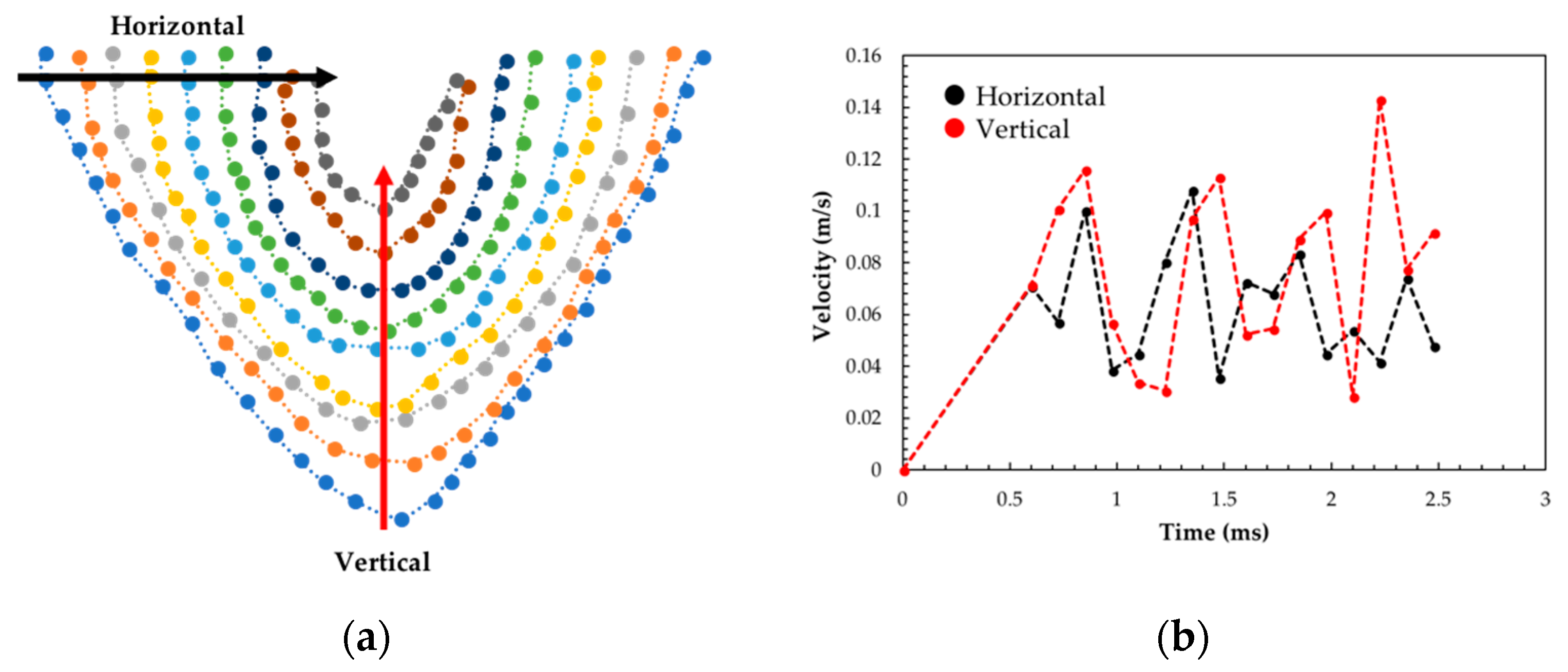
3.1. APS Experiment Melt Pool Tracking

A representative solid–liquid interface evolution during solidification and resulting solidification velocities are presented in Figure 5a,b, respectively. The approximate melt pool outlines in Figure 5a were obtained by manually plotting points along the perimeter of the observed solid–liquid interface from the in situ synchrotron X-ray radiography for a series of time steps. With this solid–liquid interface progression, velocities in any direction could be determined with those for the horizontal and vertical directions, as shown in Figure 5b. These velocities were compared to those predicted by the simulations and used to assess how well the models correlated to the experiments. Additionally, Figure 6a–c illustrates how the maximum width and depth of the melt pools were obtained from postmortem microscopy and in situ radiography of the simulated L-PBF spot-melts and rasters. These values were used to calibrate the models presented in the next section.

3.2. Melt-Pool Modeling

All spot-melt and raster scenarios were successfully modeled within SYSWELD. A representative simulation is presented below in Figure 7. The resulting dimensions of the simulated melt pools matched the experiments well, with no more than 10% error observed.

From these simulations, predicted solidification velocities were obtained horizontally at the top of the melt pool and compared to those calculated from the APS in situ radiography for the selected spot-melt and raster scenarios. Similar in situ spot-melt experiments performed by Zhao et al. on thin Ti-64 plates yielded similar velocity profiles to those presented in Figure 8a–c [24]. After the laser is shut off, no initial solidification is detected until hundreds of microseconds later. Upon the initial measurable solidification, subsequent solid–liquid interface velocities remained relatively constant throughout much of the solidification. In some instances, the velocity appears to slightly decrease, which was also noted by Zhao et al. and hypothesized to be a result of recalescence. The measured velocities in this work do not reach as high of values as reported by Zhao et al. (~0.1 m/s vs. ~0.5 m/s); however, this is likely due to slight differences in experimental conditions.

Directly comparing the experimental and simulated velocities, the first discrepancy between the solidification velocities from SYSWELD and the APS experiments is that the simulations output data at relatively coarse time-steps. This results in the simulations are unable to completely convey the solidification trends for each set of process parameters. For example, in Figure 8a, only two SYSWELD velocity measurements could be obtained, which does not allow for an accurate prediction of solidification conditions. Additionally, in some scenarios, SYSWELD predicts the melt pool is fully solidified approximately 0.5 ms before that observed in the experimental data set, as seen in Figure 8b,c. For the rasters in Figure 8d–f, the Vs obtained directly from the APS experiments reach higher values as compared to what the model predicts. These Vs are also less continuous and “jump” up or down quickly, which is likely due to the limitations of the frame rate of the camera used in the experiments and difficulty in tracking low-power melt pools. If these velocities were averaged, they would better match the expected steady-state velocities.

Although limited in some prediction capabilities, many of the simulations are able to predict the general solidification of rasters, but not spot-melts. From in situ experiments conducted using a dynamic transmission electron microscope (DTEM), Mckeown et al. showed that as the solidification front progresses in a spot-melt, it does so with a relatively constant acceleration [34]. In all three spot-melt scenarios, the predicted velocities from SYSWELD do not exhibit this linear increase. Rather, there appears to be a change from a decreasing to increasing acceleration as the laser power is increased. This suggests that the simulation is not able to capture this phenomenon. For the rasters in Figure 8d–f, a better correlation is observed, where the velocity initially increases until it reaches a steady state, where this velocity is approximately the laser travel speed. It then slightly decreases when the laser is turned off, until the velocity sharply increases again during the final stages of solidification. Once the laser is turned off, the melt pool is essentially a spot-melt and exhibits the same constant acceleration of the solid–liquid interface, as discussed above.

SYSWELD does not allow for the direct calculation of thermal gradients (Gs), so they were determined using the following relationship:

$$G=\frac{1}{V}\dot{T}$$

(2)

where V is the solidification velocity and $\dot{T}$ is the cooling rate. From Figure 9a, the G-V conditions during solidification of a 139 W spot-melt transition from higher thermal gradients and lower velocities to lower thermal gradients and higher velocities as solidification progresses. An opposite relationship is observed in Figure 9b for a 53.5 W and 0.25 m/s raster during the progression of solidification, where low Vs and Gs are initially predicted until steady-state conditions are achieved and the G-V conditions then become approximately constant. When the laser is turned off, the raster melt-pool should exhibit conditions similar to a spot-melt; however, the thermal gradient increases rather than decreases, as in the spot-melt. This inconsistency may be a result of the very low power of the raster, and the melt pool created as a result. Applying these observations to predicted grain morphologies, the solidification conditions of the spot-melt correspond to an initially fully columnar structure that transforms into a mixed structure as solidification progresses. The different G-V conditions in the raster result in an equiaxed structure that transforms to mixed morphology during the final stages of solidification.

All spot-melt and raster scenarios were successfully modeled within FLOW-3D; a representative simulation is presented below in Figure 10. The resulting dimensions of the simulated melt pools were more difficult to match to the experiments than SYSWELD, but no more than 15% error was observed. The increased complexity of FLOW-3D allowed for data output at finer time-steps, and the predicted Vs better matched the solidification characteristics of the melt pool. For the spot-melt in Figure 11a, both FLOW-3D and SYSWELD datasets agree with the experimental Vs and maintain a constant velocity of ~0.05 m/s. However, SYSWELD predicts final solidification occurs 0.5 ms before experimentally observed, while FLOW-3D better matches. At the end of solidification, FLOW-3D predicts a large increase in velocity that was not captured in the experimental dataset. This final increase was predicted in every performed FLOW-3D simulation, while if observed in the experimental data, was not to the extent of FLOW-3D. However, other rapid solidification experiments have reported this acceleration during the final stages of solidification [26,35]. Zhao et al. attributed it to the maximum local thermal gradients better aligning with the easy growth directions as the grains approach the center of the melt pool [24]. Therefore, it is likely this phenomenon did occur in the melt pool, but the limited spatial and temporal resolution of the experimental in situ imaging was unable to capture it. These results are also in good agreement with other simulation work that has examined solidification velocities of spot-melts for AM and traditional laser welding [25,36,37]. For the raster presented in Figure 11b, similar observations are seen between the three datasets. In much of the steady-state region, both FLOW-3D and SYSWELD predict an approximately constant velocity of 0.25 m/s that matches with the experimental data. There are many variations in the experimental data, but they are approximately centered around the travel speed, 0.25 m/s. These jumps are likely due to the difficulty in seeing this low-power raster, and therefore manually tracking the melt pool. Although the two predicted datasets align during the steady state, the transient conditions deviate. SYSWELD does not predict a steady state occurring until around 2 ms, where both FLOW-3D and experimental data show that it occurs earlier at 1 ms.

Predicted G-V conditions from FLOW-3D are compared to SYSWELD for the same spot-melt and raster scenario below in Figure 12. The initial solidification conditions of the spot-melt in Figure 12a deviate between the two pieces of software, where FLOW-3D predicts a much lower solidification velocity for a similar thermal gradient. Despite this difference, the same columnar grain morphology is expected using the overlaid CET. However, previous spot-melt simulation work has shown that as solidification progresses, velocity continually increases, while thermal gradients decrease [25,36,37]. These observations better align with the predictions of FLOW-3D compared to SYSWELD. As solidification progresses, the G-V conditions predicted by the two pieces of software begin to align, until the premature solidification prediction of the SYSWELD model. The acceleration of the solid/liquid interface at the final stages of solidification with FLOW-3D results in the prediction of a greater chance of forming a fully equiaxed region in the spot-melt. Raghavan et al. performed similar G-V mapping for Inconel 718 spot-melts and also found that at the later stages of solidification, the decreasing Gs and increasing Vs resulted in a greater likelihood of transitioning from columnar to equiaxed grains [25]. This change in grain morphology is also commonly observed during fusion welding [38].

Unlike the spot-melt scenario, Figure 12b shows a significant deviation between FLOW-3D and SYSWELD for predicted G-V conditions of a raster. The thermal gradients at the initial solidification of the melt pool differ by orders of magnitude. This results in a predicted columnar morphology for FLOW-3D and equiaxed for SYSWELD. The discrepancy is likely a result of FLOW-3D accounting for Marangoni flow and recoil pressure in the melt pool. Khairallah et al. showed that activating these two effects resulted in lower amounts of residual heat compared to more simplistic models that neglect those phenomena [39]. The reason for this is that Marangoni flow and recoil pressure effectively alter the cooling conditions, due to the formation of a melt pool with increased surface area, where evaporative and radiative surface cooling can then aid in increasing the cooling rate of the melt pool. As discussed previously, SYSWELD does not directly output a thermal gradient, and Equation (2) was used to indirectly obtain it from solidification velocity and cooling rate. If more simplistic models such as SYSWELD predict larger amounts of stored heat for the same process parameters, this results in slower cooling rates than those of more complicated models. This explains why SYSWELD predicts smaller thermal gradients as compared to FLOW-3D for similar velocities. As a steady state is approached within the system, both models continue to exhibit dissimilar trends. For FLOW-3D, the thermal gradient decreases before remaining relatively constant during the steady state, while the thermal gradient increases in SYSWELD. In similar modeling work conducted by Polonsky et al., the addition of fluid flow was shown to not alter the G-V trends during solidification [40]. However, this is not true in this work, although this discrepancy may be a result of how Gs were indirectly calculated, rather than directly outputted. Lastly, when the laser is turned off and solidification begins to resemble that of a spot-melt rather than a raster, FLOW-3D follows the G-V trend predicted by both models in Figure 12a, where the velocity increases as the thermal gradient slightly decreases. SYSWELD predicts the complete opposite trend and does not even match up with its own spot-melt prediction. However, this is likely due to the combination of a small melt-pool and the inability of SYSWELD to output sufficiently fine time-steps, rather than discrepancies in the same software for spot-melts and rasters. Although the final solidification conditions of the two models both predict a mixed structure, the evolution from start to finish is completely different. FLOW-3D is columnar where SYSWELD is equiaxed for much of the raster, until both transition to mixed during the final stages of solidification.

4. Conclusions

Two different simulation tools, SYSWELD and FLOW-3D, were used to model simulated L-PBF spot-melt and raster experiments performed at the APS at ANL. These experiments were used to calibrate the models and compare the accuracy of their solidification velocity predictions. From this work, drawn conclusions are as follows:

(1)

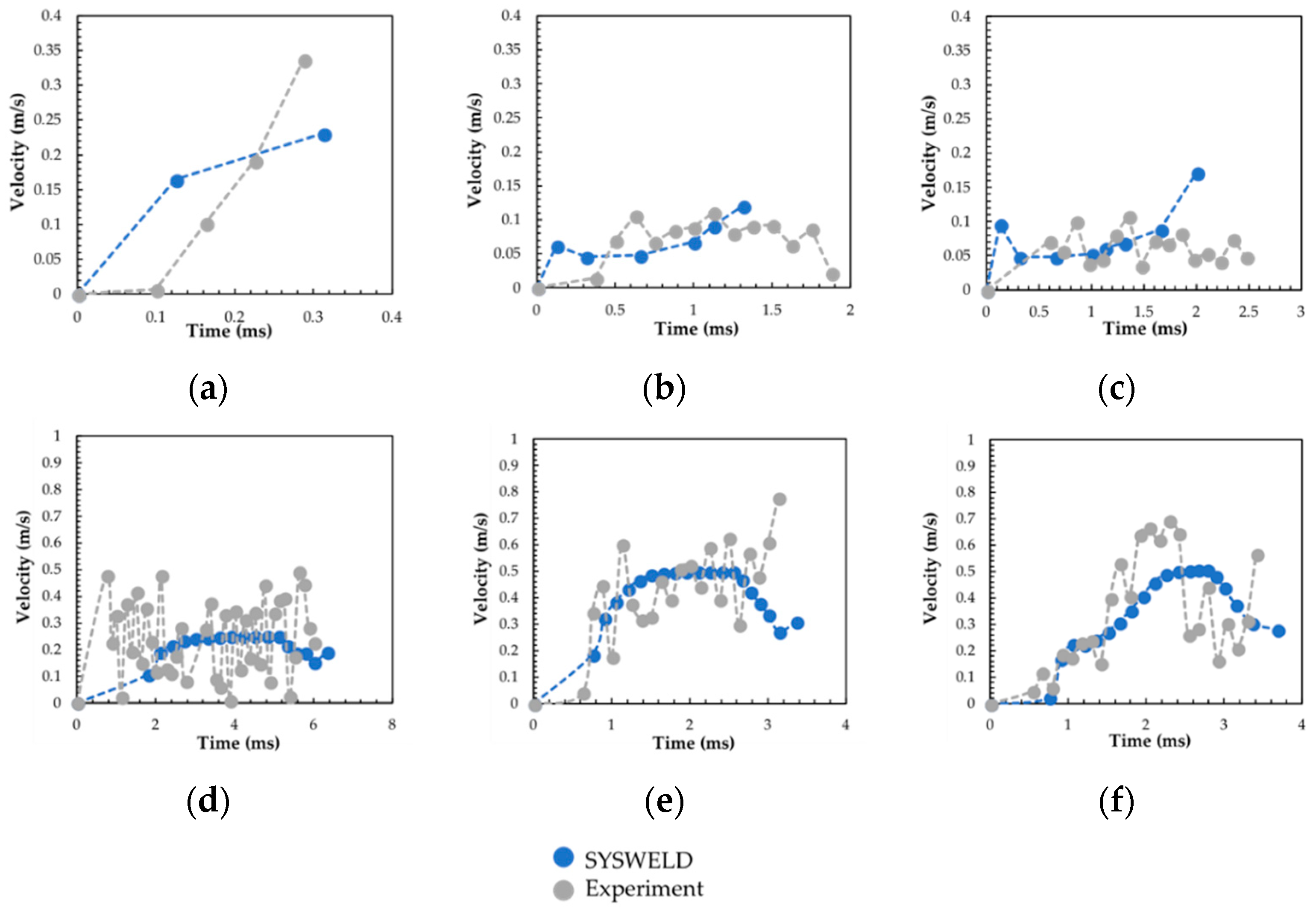
For spot-melts, model predictions from more simplistic tools such as SYSWELD are able to match velocity profiles obtained from specialized AM-simulated experiments. However, the relatively coarse time-steps make it difficult to fully capture the initial, intermediate, and final stages of melt-pool solidification.

(2)

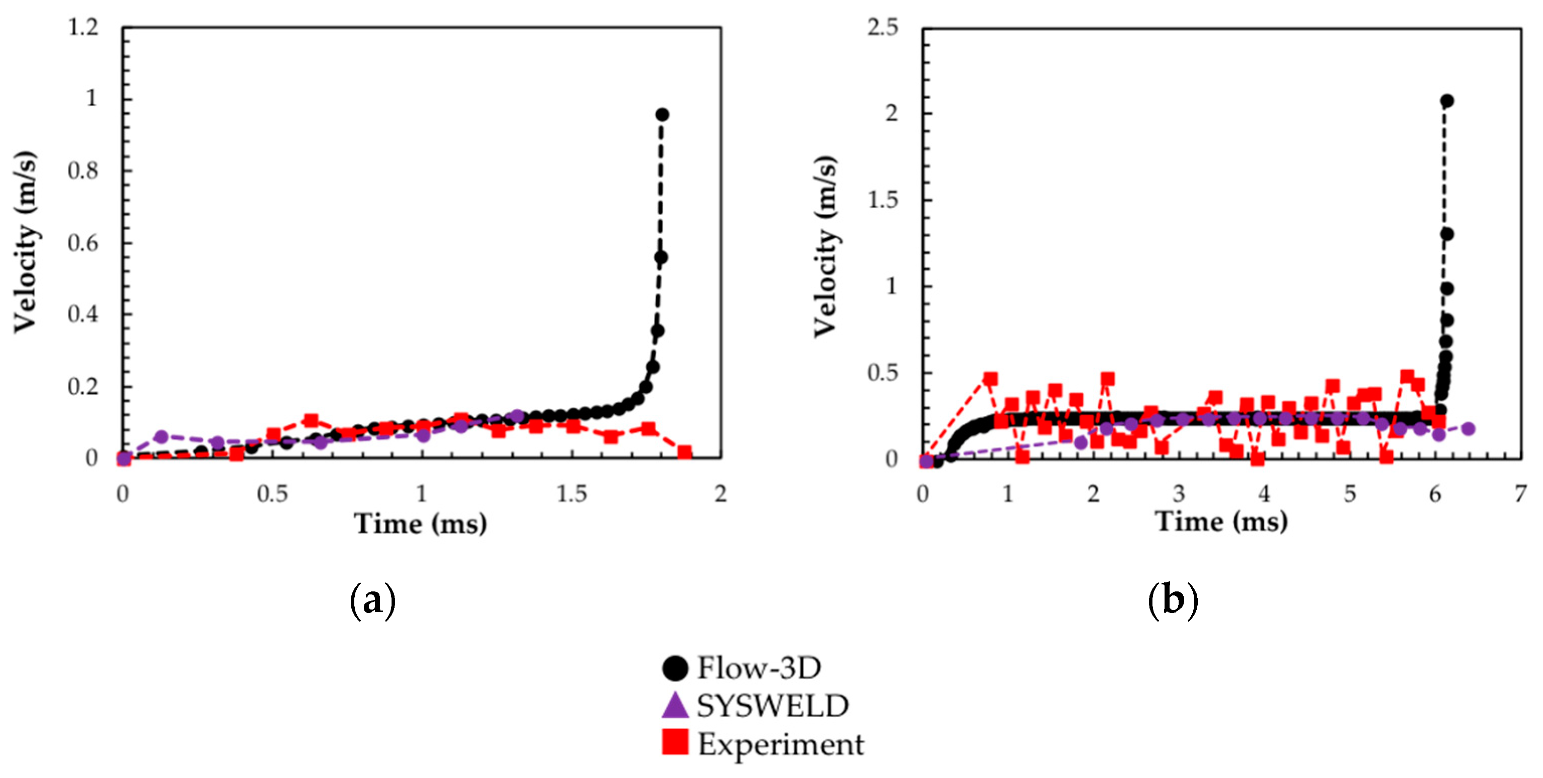
Final solidification phenomena known to occur in rapid solidification experiments, such as rapid acceleration of the solid–liquid interface, were undetectable with the utilized in situ synchrtoron x-ray imaging, but were predicted by FLOW-3D. This capability shows that high-fidelity models are able to provide insights into melt-pool solidification conditions that may not be detectable with some experimental setups.

(3)

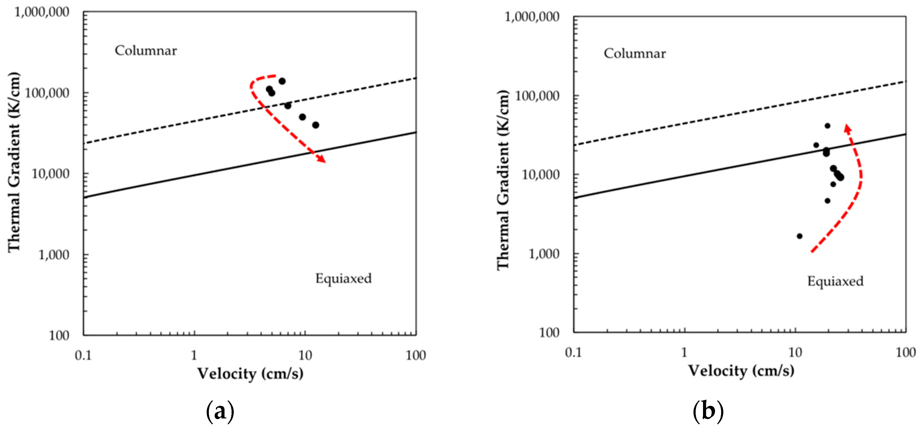
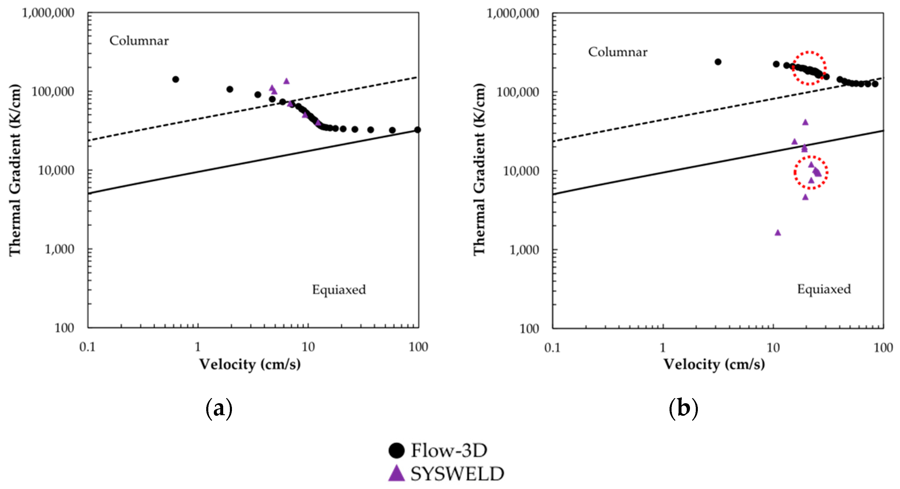
G-V predictions of spot-melts from SYSWELD and FLOW-3D align with each other and experimental observations from other work. This is not true of raster simulations, where SYSWELD predicts G-V trends different from those of FLOW-3D and basic knowledge of melt-pool solidification. This presents a limitation of SYSWELD for predicting as-built grain morphologies using solidification maps.

Without knowledge of the actual grain morphologies of these experiments, it is difficult to determine the accuracy of the G-V predictions. The use of electron backscatter diffraction (EBSD) would provide insights and validate or invalidate grain morphology predictions of the models. If validated, this approach provides a method for the determination of parameter regimes that produce desired grain morphologies. This methodology can also be applied to understand the effect of other processing parameters, such as scan strategy or preheat temperature.

Although direct comparison to as-solidified grain morphologies is still needed to validate the predictions of these models, FLOW-3D better predicts solidification conditions during L-PBF and can be utilized to advance our understanding of alloys’ response to a range of AM-like conditions.

References

1. Duerig, T.W.; Terlinde, G.T.; Williams, J.C. Phase transformations and tensile properties of Ti-10V-2Fe-3AI. Met. Mater. Trans. A 1980, 11, 1987–1998. [Google Scholar] [CrossRef]
2. Duerig, T.W.; Williams, J.C. Beta Titanium Alloys in the 80s: Proceedings of the Symposium; Metallurgical Society of AIME: Englewood, CO, USA, 1984; pp. 19–67. [Google Scholar]
3. Lütjering, G.; Williams, J.C. Titanium, 2nd ed.; Springer: Berlin/Heidelberg, Germany; New York, NY, USA, 2007. [Google Scholar]
4. Bermingham, M.; StJohn, D.; Krynen, J.; Tedman-Jones, S.; Dargusch, M. Promoting the columnar to equiaxed transition and grain refinement of titanium alloys during additive manufacturing. Acta Mater. 2019, 168, 261–274. [Google Scholar] [CrossRef]
5. Roehling, T.T.; Shi, R.; Khairallah, S.A.; Roehling, J.D.; Guss, G.M.; McKeown, J.T.; Matthews, M.J. Controlling grain nucleation and morphology by laser beam shaping in metal additive manufacturing. Mater. Des. 2020, 195, 109071. [Google Scholar] [CrossRef]
6. Qiu, C.; Ravi, G.; Attallah, M.M. Microstructural control during direct laser deposition of a β-titanium alloy. Mater. Des. 2015, 81, 21–30. [Google Scholar] [CrossRef]
7. Zhu, Y.-Y.; Tang, H.-B.; Li, Z.; Xu, C.; He, B. Solidification behavior and grain morphology of laser additive manufacturing titanium alloys. J. Alloy. Compd. 2018, 777, 712–716. [Google Scholar] [CrossRef]
8. Balla, V.K.; Das, M.; Mohammad, A.; Al-Ahmari, A.M. Additive Manufacturing of γ-TiAl: Processing, Microstructure, and Properties: Additive Manufacturing of γ-TiAl: Processing. Adv. Eng. Mater. 2016, 18, 1208–1215. [Google Scholar] [CrossRef]
9. Kurzynowski, T.; Gruber, K.; Stopyra, W.; Kuźnicka, B.; Chlebus, E. Correlation between process parameters, microstructure and properties of 316 L stainless steel processed by selective laser melting. Mater. Sci. Eng. A 2018, 718, 64–73. [Google Scholar] [CrossRef]
10. Liang, Y.-J.; Cheng, X.; Li, J.; Wang, H.-M. Microstructural control during laser additive manufacturing of single-crystal nickel-base superalloys: New processing–microstructure maps involving powder feeding. Mater. Des. 2017, 130, 197–207. [Google Scholar] [CrossRef]
11. Yang, J.; Yu, H.; Yin, J.; Gao, M.; Wang, Z.; Zeng, X. Formation and control of martensite in Ti-6Al-4V alloy produced by selective laser melting. Mater. Des. 2016, 108, 308–318. [Google Scholar] [CrossRef]
12. Zhai, Y.; Galarraga, H.; Lados, D.A. Microstructure, static properties, and fatigue crack growth mechanisms in Ti-6Al-4V fabricated by additive manufacturing: LENS and EBM. Eng. Fail. Anal. 2016, 69, 3–14. [Google Scholar] [CrossRef]
13. Thijs, L.; Verhaeghe, F.; Craeghs, T.; Van Humbeeck, J.; Kruth, J.-P. A study of the microstructural evolution during selective laser melting of Ti–6Al–4V. Acta Mater. 2010, 58, 3303–3312. [Google Scholar] [CrossRef]
14. Levkulich, N.; Semiatin, S.; Gockel, J.; Middendorf, J.; DeWald, A.; Klingbeil, N. The effect of process parameters on residual stress evolution and distortion in the laser powder bed fusion of Ti-6Al-4V. Addit. Manuf. 2019, 28, 475–484. [Google Scholar] [CrossRef]
15. Saville, A.I.; Vogel, S.C.; Creuziger, A.; Benzing, J.T.; Pilchak, A.L.; Nandwana, P.; Klemm-Toole, J.; Clarke, K.D.; Semiatin, S.L.; Clarke, A.J. Texture evolution as a function of scan strategy and build height in electron beam melted Ti-6Al-4V. Addit. Manuf. 2021, 46, 102118. [Google Scholar] [CrossRef]
16. Norsk Titanium Delivers First FAA-Certified, Additive Manufactured Ti64 Structural Aviation Components. Available online: http://www.norsktitanium.com/media/press/norsk-titanium-delivers-first-faacertified-additive-manufactured-ti64-structural-aviation-components (accessed on 20 October 2021).
17. Zopp, C.; Blümer, S.; Schubert, F.; Kroll, L. Processing of a metastable titanium alloy (Ti-5553) by selective laser melting. Ain Shams Eng. J. 2017, 8, 475–479. [Google Scholar] [CrossRef] [Green Version]
18. Schwab, H.; Palm, F.; Kühn, U.; Eckert, J. Microstructure and mechanical properties of the near-beta titanium alloy Ti-5553 processed by selective laser melting. Mater. Des. 2016, 105, 75–80. [Google Scholar] [CrossRef]
19. Dehoff, R.; Kirka, M.M.; Sames, W.J.; Bilheux, H.; Tremsin, A.; Lowe, L.E.; Babu, S. Site specific control of crystallographic grain orientation through electron beam additive manufacturing. Mater. Sci. Technol. 2014, 31, 931–938. [Google Scholar] [CrossRef]
20. Plotkowski, A.; Ferguson, J.; Stump, B.; Halsey, W.; Paquit, V.; Joslin, C.; Babu, S.; Rossy, A.M.; Kirka, M.; Dehoff, R. A stochastic scan strategy for grain structure control in complex geometries using electron beam powder bed fusion. Addit. Manuf. 2021, 46, 102092. [Google Scholar] [CrossRef]
21. Kobryn, P.; Semiatin, S. Microstructure and texture evolution during solidification processing of Ti–6Al–4V. J. Mater. Process. Technol. 2003, 135, 330–339. [Google Scholar] [CrossRef]
22. DebRoy, T.; Wei, H.L.; Zuback, J.S.; Mukherjee, T.; Elmer, J.W.; Milewski, J.O.; Beese, A.M.; Wilson-Heid, A.; De, A.; Zhang, W. Additive manufacturing of metallic components–Process, structure and properties. Prog. Mater. Sci. 2018, 92, 112–224. [Google Scholar] [CrossRef]
23. Al-Bermani, S.S.; Blackmore, M.L.; Zhang, W.; Todd, I. The Origin of Microstructural Diversity, Texture, and Mechanical Properties in Electron Beam Melted Ti-6Al-4V. Met. Mater. Trans. A 2010, 41, 3422–3434. [Google Scholar] [CrossRef]
24. Zhao, C.; Fezzaa, K.; Cunningham, R.W.; Wen, H.; De Carlo, F.; Chen, L.; Rollett, A.D.; Sun, T. Real-time monitoring of laser powder bed fusion process using high-speed X-ray imaging and diffraction. Sci. Rep. 2017, 7, 3602. [Google Scholar] [CrossRef] [PubMed]
25. Raghavan, N.; Dehoff, R.; Pannala, S.; Simunovic, S.; Kirka, M.; Turner, J.; Carlson, N.; Babu, S.S. Numerical modeling of heat-transfer and the influence of process parameters on tailoring the grain morphology of IN718 in electron beam additive manufacturing. Acta Mater. 2016, 112, 303–314. [Google Scholar] [CrossRef] [Green Version]
26. Mills, K.C. Recommended Values of Thermophysical Properties for Selected Commercial Alloys; Woodhead: Cambridge, UK, 2002. [Google Scholar] [CrossRef]
27. Thermo-Calc Software TCTI/Ti-Alloys Database Version 3.
28. Bayat, M.; Thanki, A.; Mohanty, S.; Witvrouw, A.; Yang, S.; Thorborg, J.; Tiedje, N.S.; Hattel, J. Keyhole-induced porosities in Laser-based Powder Bed Fusion (L-PBF) of Ti6Al4V: High-fidelity modelling and experimental validation. Addit. Manuf. 2019, 30, 100835. [Google Scholar] [CrossRef]
29. Kurz, W.; Giovanola, B.; Trivedi, R. Theory of microstructural development during rapid solidification. Acta Met. 1986, 34, 823–830. [Google Scholar] [CrossRef]
30. Gäumann, M.; Bezençon, C.; Canalis, P.; Kurz, W. Single-crystal laser deposition of superalloys: Processing–microstructure maps. Acta Mater. 2001, 49, 1051–1062. [Google Scholar] [CrossRef]
31. Liu, D.; Wang, Y. Mesoscale multi-physics simulation of rapid solidification of Ti-6Al-4V alloy. Addit. Manuf. 2018, 25, 551–562. [Google Scholar] [CrossRef]
32. Rolchigo, M.; LeSar, R. Modeling of binary alloy solidification under conditions representative of Additive Manufacturing. Comput. Mater. Sci. 2018, 150, 535–545. [Google Scholar] [CrossRef]
33. Hunt, J. Steady state columnar and equiaxed growth of dendrites and eutectic. Mater. Sci. Eng. 1984, 65, 75–83. [Google Scholar] [CrossRef]
34. McKeown, J.T.; Zweiacker, K.; Liu, C.; Coughlin, D.R.; Clarke, A.J.; Baldwin, J.K.; Gibbs, J.; Roehling, J.D.; Imhoff, S.D.; Gibbs, P.J.; et al. Time-Resolved In Situ Measurements During Rapid Alloy Solidification: Experimental Insight for Additive Manufacturing. JOM 2016, 68, 985–999. [Google Scholar] [CrossRef]
35. McKeown, J.T.; Kulovits, A.K.; Liu, C.; Zweiacker, K.; Reed, B.W.; LaGrange, T.; Wiezorek, J.M.; Campbell, G.H. In situ transmission electron microscopy of crystal growth-mode transitions during rapid solidification of a hypoeutectic Al–Cu alloy. Acta Mater. 2014, 65, 56–68. [Google Scholar] [CrossRef]
36. He, X.; Fuerschbach, P.W.; DebRoy, T. Heat transfer and fluid flow during laser spot welding of 304 stainless steel. J. Phys. D Appl. Phys. 2003, 36, 1388–1398. [Google Scholar] [CrossRef]
37. He, X.; Elmer, J.W.; DebRoy, T. Heat transfer and fluid flow in laser microwelding. J. Appl. Phys. 2005, 97, 084909. [Google Scholar] [CrossRef]
38. Lienert, T.; Siewert, T.; Babu, S.; Acoff, V. (Eds.) Fundamentals of Weld Solidification. In Welding Fundamentals and Processes; ASM International: Almere, The Netherlands, 2011; pp. 96–114. [Google Scholar] [CrossRef]
39. Khairallah, S.A.; Anderson, A.T.; Rubenchik, A.; King, W.E. Laser powder-bed fusion additive manufacturing: Physics of complex melt flow and formation mechanisms of pores, spatter, and denudation zones. Acta Mater. 2016, 108, 36–45. [Google Scholar] [CrossRef] [Green Version]
40. Polonsky, A.T.; Raghavan, N.; Echlin, M.P.; Kirka, M.M.; Dehoff, R.R.; Pollock, T.M. 3D Characterization of the Columnar-to-Equiaxed Transition in Additively Manufactured Inconel 718. In Superalloys 2020; Tin, S., Hardy, M., Clews, J., Cormier, J., Feng, Q., Marcin, J., O’Brien, C., Suzuki, A., Eds.; Springer International Publishing: Cham, Switzerland, 2020; pp. 990–1002. [Google Scholar] [CrossRef]
Figure 1. Schematic of the X-ray imaging L-PBF simulator experiments on the Sector 32-ID-B beamline at the APS at ANL. Note: distances between components not to scale.
Metals 12 01217 g001
Figure 2. Graphs of estimated (a) density, (b) thermal conductivity, and (c) specific heat as a function of temperature for Ti-1023.
Metals 12 01217 g002
Figure 3. Dimensioned computer-aided design (CAD) model used within SYSWELD for all spot-melt and raster scenarios.
Metals 12 01217 g003
Figure 4. Dimensioned CAD model used within FLOW-3D with labeled boundary conditions for all spot-melt and raster scenarios.
Metals 12 01217 g004
Figure 5. (a) Progression of the solid–liquid interface of a spot-melt for a series of 0.25 ms time-steps with labeled directions of velocity extraction; (b) solidification velocities as a function of time in the horizontal and vertical directions of the spot-melt presented in (a).
Metals 12 01217 g005
Figure 6. Methods of obtaining melt pool dimensions for calibration of model for (a) maximum width of a spot-melt using top-down, postmortem secondary electron imaging (SEI), (b) maximum depth of a spot-melt using in situ imaging, and (c) width and depth of a raster using in situ imaging.
Metals 12 01217 g006
Figure 7. Cross-section of 82 W spot-melt scenario, showing maximum temperature contours predicted by SYSWELD and resulting maximum melt pool depth and width. Note: grey area shows predicted area that is above 1610 °C, the approximate liquidus temperature.
Metals 12 01217 g007
Figure 8. Plots of predicted solidification velocity at the top of the melt pool for (a) 82 W, (b) 139 W, and (c) 197 W spot-melts and (d) 53.5 W and 0.25 m/s, (e) 82 W and 0.5 m/s, and (f) 139 W and 0.5 m/s rasters using SYSWELD and values obtained from X-ray in situ radiography. Note: time = 0 for (ac) refers to the moment the laser was turned off and time = 0 for (df) refers to the moment the laser was turned on and began rastering.
Metals 12 01217 g008
Figure 9. Predicted SYSWELD G-V conditions from the edge to the center of a melt pool or beginning to end of a raster overlaid onto the Ti-1023 CET for (a) 139 W spot-melt and (b) 53.5 W and 0.25 m/s raster. Note: arrows in (a,b) show progression of solidification.
Metals 12 01217 g009
Figure 10. Cross-section of 82 W spot-melt scenario, showing maximum melt region predicted by FLOW-3D and the resulting melt pool depth and width.
Metals 12 01217 g010
Figure 11. Comparison of solidification velocity at the top of the melt pool predicted by FLOW-3D and SYSWELD and observed in the experiment for (a) 139 W spot-melt and (b) 53.5 W and 0.25 m/s raster. Note: time = 0 for (a) refers to the moment the laser was turned off and time = 0 for (b) refers to the moment the laser was turned on and began rastering. Additionally, the laser was turned off at 6 ms in (b).
Metals 12 01217 g011
Figure 12. Predicted FLOW-3D and SYSWELD G-V conditions at the top of the melt pool overlaid onto the Ti-1023 CET for (a) 139 W spot-melt and (b) 53.5 W and 0.25 m/s raster. Note: circles in (b) show the steady-state regions.
Metals 12 01217 g012