Comparison of Modified Johnson–Cook Model and Strain–Compensated Arrhenius Constitutive Model for 5CrNiMoV Steel during Compression around Austenitic Temperature

Abstract

Isothermal compression behaviors of 5CrNiMoV steel were studied at temperatures of 870, 800, 750, and 700 °C, with strain rates of 0.001, 0.005, 0.01, 0.05, and 0.1 s⁻¹, the compression temperatures 870 and 800 °C are above Ac3, as well as 750 and 700 °C below Ac3 temperature. The Modified Johnson–Cook (MJC) model and the Strain–Compensated Arrhenius (SCA) model were employed to demonstrate the relationship between the flow stress and the compression parameters. The correlation coefficient (R) and average absolute relative error (AARE) between the calculational and experimental flow stress were used to evaluate the accuracy of the two models. The results show that the effect of dynamic softening on flow stress is much more significant at higher temperatures and lower strain rates, while this effect is not obvious when the strain rate exceeds 0.005 s⁻¹ with the temperature below Ac3. The MJC model has a good accuracy close to the reference conditions (0.001 s⁻¹ and 700 °C), and it is suitable to predict the plastic behavior when the flow stress is lower than 200 Mpa. The unbiased AARE values were 6.82 and 5.71 for MJC model and SCA model, respectively, which implied the SCA model has a higher accuracy than the MJC model. The SCA model was believed to be capable of being used to illustrate the thermomechanical behavior of 5CrNiMoV tool steel in a wide range of plastic deformation conditions.

1. Introduction

Hot working tool steels are mainly used in the production of various dies that are employed at elevated temperature, such as hammer forging die, hot extrusion die, machine forging die, and casting die. Because its working conditions are extremely harsh and complex, high strength, toughness, and good wear resistance are required [1,2,3]. To satisfy these requirements, searching for new alloys with additional alloying elements and using a reasonable hot working process have always attracted significant attention [4,5,6].

The stress–strain curve of metallic materials plays an important role, not only for designing deformation parameters but also for performing nonlinear finite element numerical simulation to solve an elastoplastic deformation problem [7,8]. Generally, there are two methods to obtain a stress–strain curve at a predefined temperature and strain rate. Conventional methods including tensile or compression tests, and then converting from engineering stress–strain data to true stress–strain data [7,9]. The other uses finite element simulations or calculational/artificial neural network methods to predict the stress–strain curves [10,11,12,13]. For the sake of obtaining more reliable results, experimental measurements, in conjunction with finite element analysis, are usually performed and verify each other [10,14]. The methods are mainly dependent on the material characteristics and the strain range needs to be considered [7]. For an elastic analysis, only Poisson’s ratio and elastic modulus are required. In contrast to elastoplastic problems, additional information, such as uniaxial true stress–strain, is needed, especially in the field of large deformation and phase transformation plasticity, where the relationship among the stress, strain, and temperature is complex [11,15,16]. Many researchers have tried to illustrate the stress–strain relations, strain hardening, and dynamic softening behavior of metallic metals during plastic deformation. The stress–strain curve is the most basic and important data. Moreover, reliable numerical simulation for forging, rolling, heat-treatment, and welding always requires an accurate stress–strain curve [16,17]. The constitutive models, including empirical equation, semi-empirical equation, and physical-based equation [18], were used to illustrate the deformation behavior of metallic alloys and demonstrate the relationship among flow stress, temperature, strain, and strain rate. In these empirical and semi-empirical constitutive models, the original Johnson–Cook (JC) model [19,20,21], Modified Johnson–Cook (MJC) model [22,23,24] and Arrhenius-type model [25,26,27] are widely used in metallic alloys, such as steel alloys [25,28,29], aluminum alloys [30,31,32], magnesium alloys [33,34,35], titanium alloys [20,21], and superalloys [26,36,37], within a widely range of deformation temperature and strain rate, such as from 0.0001 [29] to 11,000 [37] s⁻¹. Gupta et al. [12] established the constitutive models to predict the flow stress of 316 austenitic stainless steel by using JC model, modified Zerilli–Armstrong model, Arrhenius Model, and artificial neural network model. The results indicated that the modified Zerilli–Armstrong model and Arrhenius Model had better accuracy in comparison with the JC model; the artificial neural network model also presented a higher value of correlation coefficient, but it is difficult to integrate with FEM software. He et al. [16] found that the compressive flow stress of 20CrMo alloy steel predicted using JC model did not agree well with the experimental values compared to MJC and Arrhenius-type model, because the couple effects of temperature and strain rate were not considered in the JC model. Tan et al. [23] proposed a MJC model and used it to describe the flow behavior of 7050-T7451 aluminum alloy, and proved that the MJC model had a better agreement than the original JC and Khan-Liu model.

The thermomechanical response of steel alloys around Ac3 temperature is vital in the hot working process, especially in the forging and heat-treatment process of forgings with large section. However, most of the studies focused on the establishment of constitutive models to analyze the relationship between stress and stain with a microstructure of single/stable phase, the thermomechanical response of the steel alloys which have an unstable microstructure (supercooled austenite) below Ac3 was seldom mentioned. In this paper, single-pass isothermal compression tests of hot working tool steel 5CrNiMoV were carried out at temperatures ranging from 700 to 870 °C with strain rates ranging from 0.001 to 0.1 s⁻¹. The compression temperatures 870 and 800 °C are above Ac3, as well as 750 and 700 °C below Ac3 temperature. The MJC model and SCA model were employed to describe the relationship among flow stress, temperature, strain, and strain rate. To evaluate the prediction accuracy of the two models, the correlation coefficient (R) and the average absolute relative error (AARE) were calculated subsequently.

2. Materials and Experiments

The chemical composition of 5CrNiMoV steel used in this study is given in

Table 1. Chemical composition of the studied 5CrNiMoV steel (wt.%).

Composition	C	Cr	Mn	Mo	Ni	V	Si	Cu	Co	Al	Fe
wt.%	0.6	0.91	0.66	0.35	1.66	0.077	0.24	0.109	0.017	0.006	Bal.

. The microstructure of the as-received forged steel mainly consists of ferrite and cementite. Thermal expansion tests were carried out using a DIL 805A dilatometer machine (TA Instruments, Hüllhorst, Germany), and cylindrical samples with a diameter of 4 mm and length of 10 mm were used. The single-pass isothermal compression tests were conducted using a thermomechanical test machine DIL 805D (TA Instruments, Hüllhorst, Germany), and the specimens have a diameter of 5 mm and length of 10 mm. A type S (Pt-Pt/Rh10%) thermocouple was spot welded in the center of the specimen surface and used for a closed-loop control of the specimen temperature. Cylindrical samples in thermal expansion and isothermal compression tests were heated by induction and cooled using inert gas. The cooling gas was ejected from the holes of the induction coil and directly meet the surface of the sample, meanwhile the temperature of the sample was controlled by adjusting the heating power and gas intensity automatically.

The isothermal compression procedure and experimental setup are shown in Figure 1. All specimens were heated to austenite homogenization temperature (870 °C) with a heating rate of 2 K/s, hold for 10 min to obtain a uniform microstructure, and then quenched to the deformation temperature with a cooling rate of 40 K/s. The specimens were individually compressed uniaxially up to a total true strain of 1.1 at 870, 800, 750, and 700 °C, with a strain rate of 0.001, 0.005, 0.01, 0.05, and 0.1 s⁻¹. The deformed specimens were quenched to room temperature after isothermal compression, with a cooling rate of 40 K/s and cooling media of helium.

The isothermal compression experimental data including time, temperature, strain, true strain, force, true stress, change of length, induction heating power, and gas cooling intensity, etc., were recorded simultaneously alongside the test. It should be noted that the deformation stamps that DIL 805D used are made of Si3N4, and the maximum force is 20 KN for safety reasons [38]. The load provided by DIL 805D is relatively limited compared to the commonly used thermomechanical test machines Gleeble 3500/3800, whose maximum compressive loads are 100 KN and 200 KN, respectively [39]. That is why when the compression test performed at lower deformation temperature and higher strain rate, such as 700 °C and 0.1 s⁻¹ in the test matrix, only a true strain of 0.8 was reached.

The compressed samples were sectioned, grinded, polished, and etched using the standard metallographic method. TESCAN VEGA3 scanning electron microscopic (SEM) (Tescan, Brno-Kohoutovice, Czech Republic) with secondary electron (SE) and back-scattering electron (BSE) mode was used for microstructure observation.

3. Results and Discussion

The dilatometer test results show that the austenitic transformation start temperature (Ac1) is 729 °C and the end temperature (Ac3) is 758 °C, when the heating rate is 0.05 K/s. The detailed temperature–dilatometer curves corresponding to different heating rates ranging from 0.05 to 50 K/s are not shown here. For specimens without external stress, temperature is the main driving force of phase transformation, the heating rate is a major factor affecting the phase transformation kinetics. Different heating rates and chemical compositions result in different Ac1 and Ac3. As is shown by the findings reported by Huang [1], where the transformation temperatures of Ac1 and Ac3 for 5CrNiMoV steel were 730 °C and 765 °C, respectively. Thus, the isothermal compression temperatures 870 °C and 800 °C are above the Ac3, as well as 750 °C and 700 °C below the Ac3. The microstructure of steel alloys is mainly austenite and phase transformation does not happen when the holding temperature above Ac3. Alloy element diffusion, grain growths, and dislocation density decreases may happen, but austenite is stable and the lattice type of the metal matrix does not change in this stage from the point of view of thermodynamics [15]. When the holding temperature is below Ac3, the microstructure is supercooled austenite which is not stable anymore and is prone to decomposition and transforming into pearlite, bainite, or martensite, resulting in the thermomechanical analysis being more complicated [5,15]. The isothermal phase transformation curves obtained using DIL 805A dilatometer confirmed that the undercooled-austenite was stable and the incubation time was enough for a compression test at different strain rates, which means the supercooled austenite did not decompose when the compressed temperature was 750 °C or 700 °C.

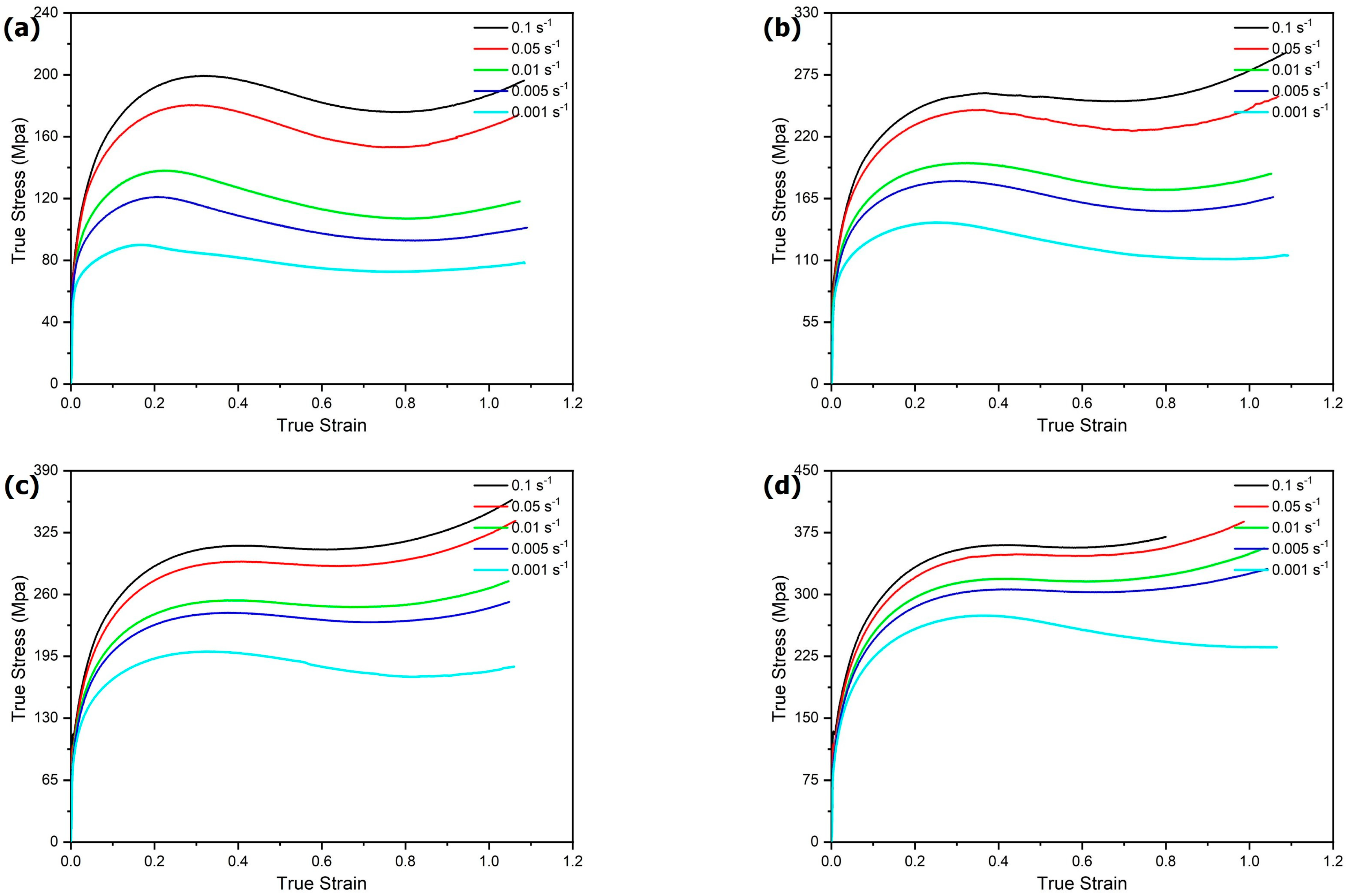
3.1. True Stress–Strain Curves of the 5CrNiMoV Steel

The true stress–strain curves of 5CrNiMoV steel under different compression conditions are shown in Figure 2. It can be seen that the deformation temperature and strain rate have a significant effect on the flow stress, similar results have also been reported by other scholars [12,28,33], despite being above or below Ac3 temperature. The flow stress increases with the increase in the strain rate or the decrease in the deformation temperature. The strain rate and true strain are the main influencing factors for work hardening, as well as temperature for dynamic softening which includes dynamic recovery and dynamic recrystallization. The true stress–strain curve can be roughly divided into three parts. The flow stress increases steeply until the true strain reached 0.1, and then gradually increased to the maximum point is the first part. Within this part, the work hardening effect dominates the flow stress in the early stage and then is counterbalanced by the dynamic softening. As the true strain increases continuously, the flow stress decreased from the maximum point gradually before the true strain reached nearly 0.8. The effect of strain-induced work hardening on the flow stress faded while the effect of dynamic softening enhanced at the same time. The strain larger than about 0.8 belongs to the third part and the flow stress increases slowly again, until the total strain reached the predefined value of 1.1.

The stress–strain curve of the isothermal compression test depends on two competing factors, work hardening and dynamic softening. The competing mechanisms can be found in many metallic materials, such as steel [19,22,28], aluminum [31,32] and titanium alloys [21,40], etc. That is why the true stress–strain curves of 5CrNiMoV steel are similar to the sine curve. It should be noted that the effect of dynamic softening on flow stress is much more significant at a higher temperature and lower strain rate, especially when the compression temperature is above Ac3, but the dynamic softening effect is not obvious when the strain rate is higher than 0.005 s⁻¹ with the compression temperature below Ac3. Even at a constant compression temperature, the true strain that corresponds to the maximum flow stress decreases with the decreasing strain rate. In contrast to the work hardening effect, which is much more obvious at lower temperatures and higher strain rates. The softening mechanism of metallic alloys usually contains dynamic recovery and continuous/discontinuous recrystallization, which depends on the alloy grade and the microstructure within it [41]. Thermal vibration and thermal diffusivity of the alloying element atom are enhanced at an elevated temperature, in addition to the stored energy accumulated with the strain, the driving force is adequate for dislocation cross-slip and climb, which lead to dynamic softening accompanied by lower flow stress. The dynamic softening is influenced by the time required to complete the corresponding true strain. If the strain rate is large enough and higher than 100 s⁻¹, that usually can be seen in Split Hopkinson Pressure Bar tests, dynamic softening during deformation is not obvious any more [23,34,37]. With the increase in strain, dislocations generation, slip, multiplication, and pile-up can be found in the deformed alloy, which leads to work hardening and an increase in flow stress [18].

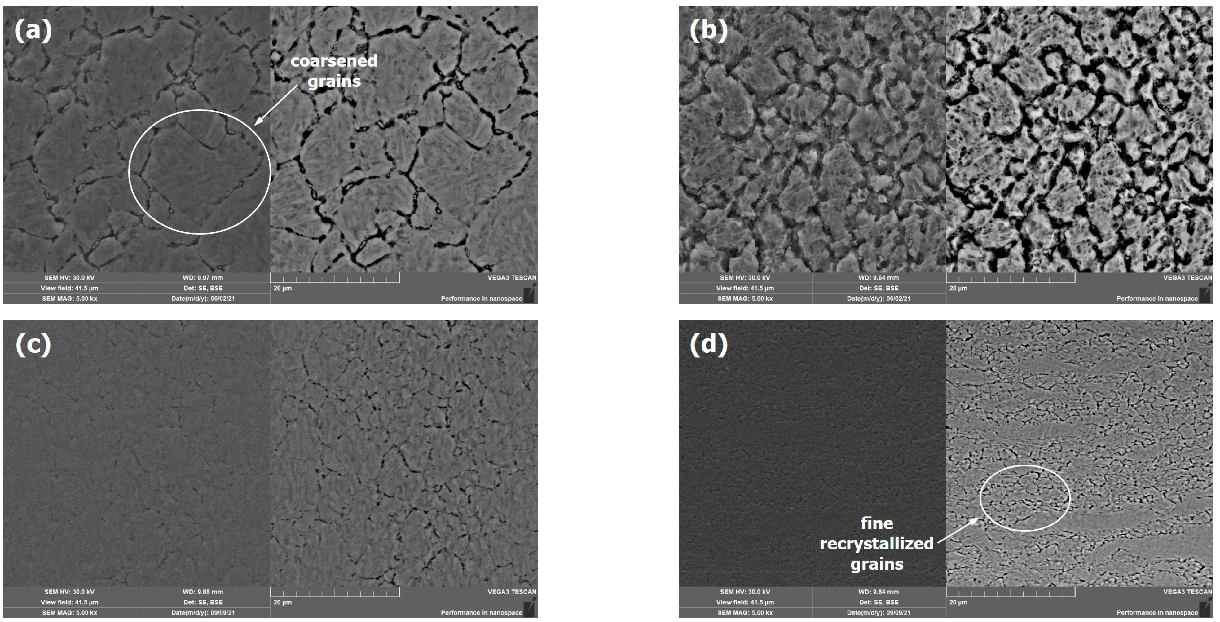
3.2. Microstructures of the 5CrNiMoV Steel after Compression

The microstructure of the as-compressed samples that deformed with a constant strain rate 0.05 s⁻¹ and different temperatures are shown in Figure 3. At temperatures below 750 °C, it is observed that the grains were severely deformed and presented as a continuous strip, few recrystallizations were found. With the increase in deformation temperature, fine recrystallized grains can be observed at the grain boundaries (Figure 3c) and their size increases gradually (Figure 3d). It should be mentioned that the cooling velocity after compression was 40 K/s, which is much higher than the critical cooling velocity for martensite transformation. If the effect of stress/strain-induced austenite decomposition can be ignored, the microstructure of the 5CrNiMoV steel should be martensite after cooling, no precipitation occurred in this process. It is implied that the dynamic softening phenomena were not significant when the compression temperature is lower than 750 °C, which is consistent with the results derived from the red stress–strain curves in Figure 2.

The SEM morphologies of the 5CrNiMoV steel compressed at 870 °C with different strain rates can be seen in Figure 3d and Figure 4. The corresponding true stress–strain curves are shown in Figure 2a. The grain size decreases with the increase in the strain rate because the grains have enough time to grow up when the specimen was compressed at a lower strain rate, which results in dynamic softening and lower flow stress. When the strain rate was 0.1 s⁻¹, fine recrystallized grains can be found (Figure 4d), recrystallization has been completed, and the flow stress raised again. The flow stress is not only influenced by the temperature, but also the grain size. That is why the stress–strain curve is dependent on the work hardening and dynamic softening.

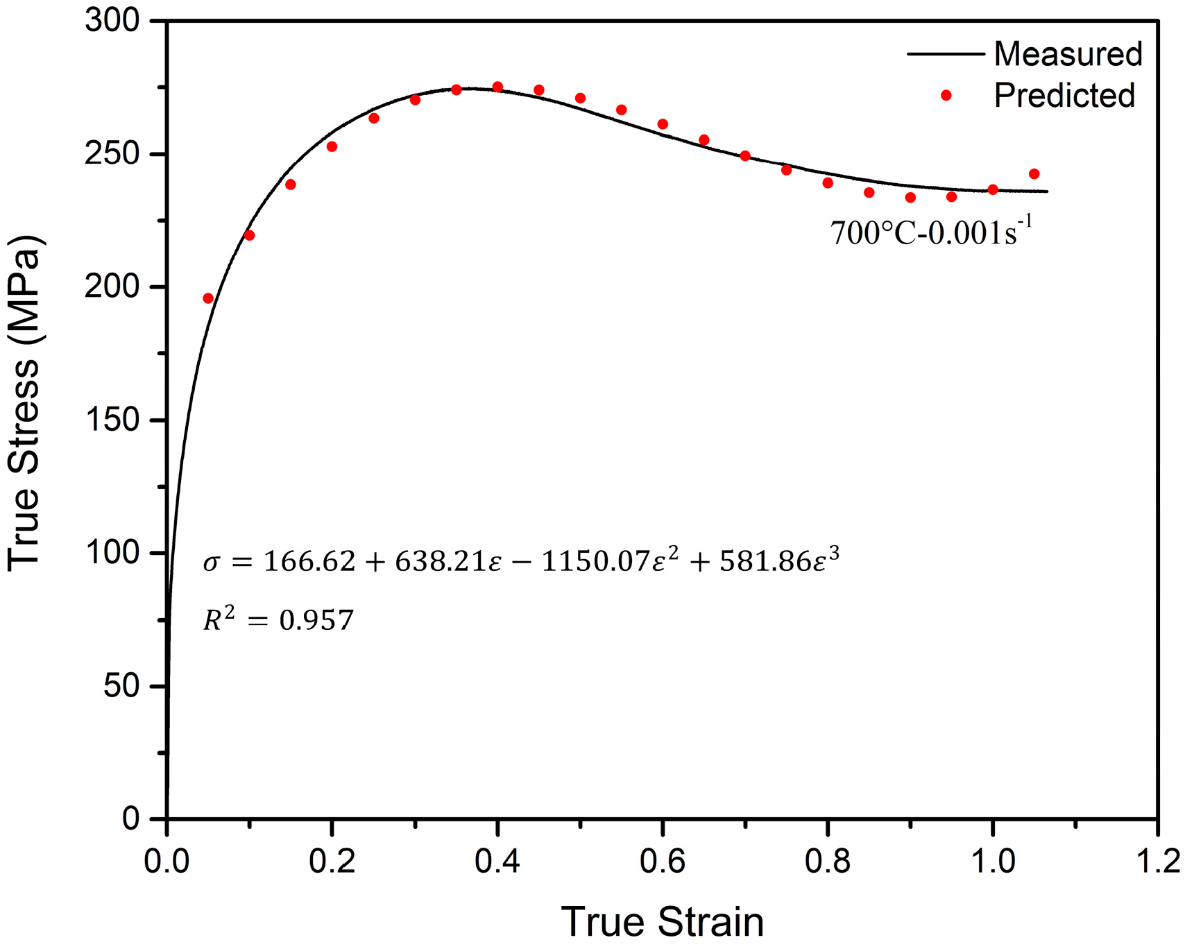
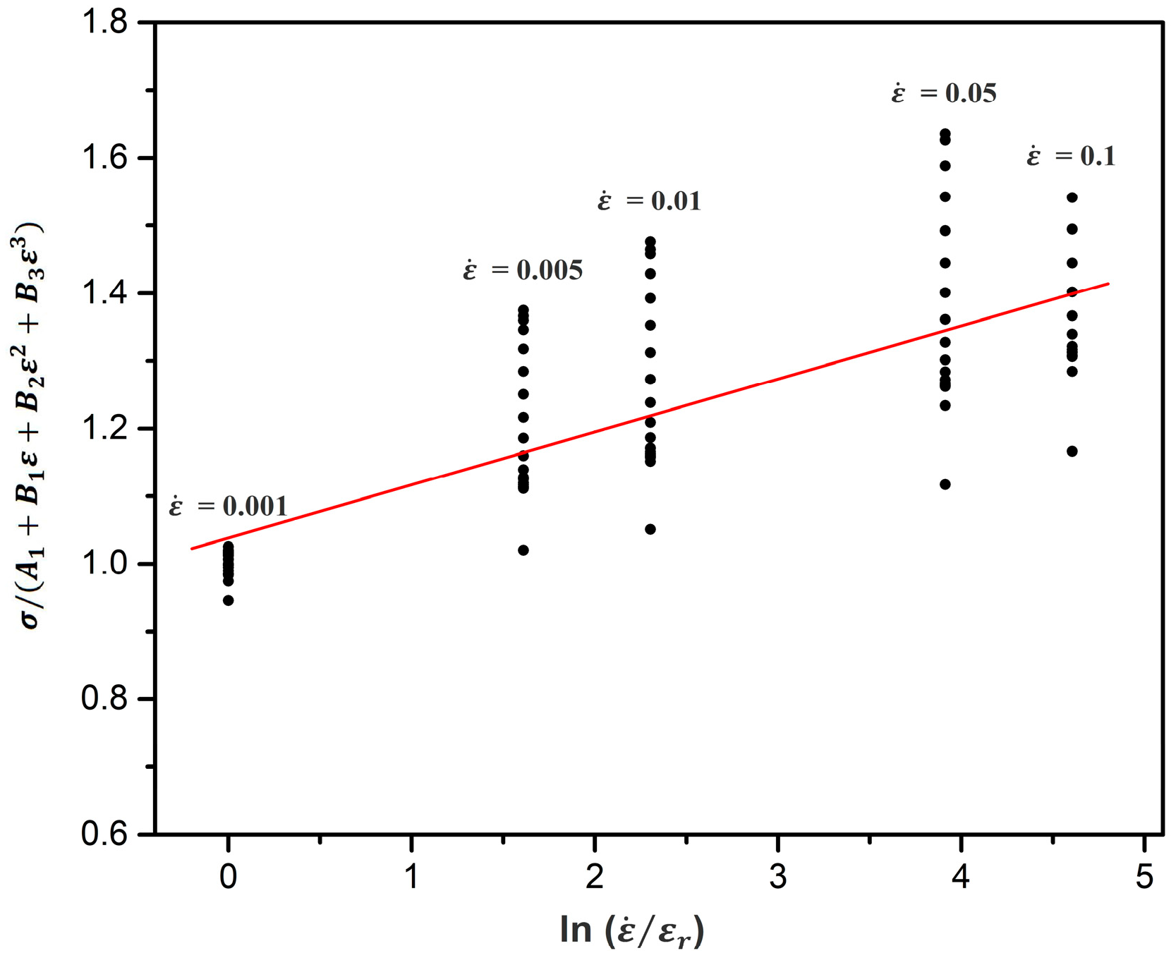
3.3. Modified Johnson–Cook Model

The JC constitutive model was first proposed by Johnson and Cook in 1983 to illustrate the relationship among stress, strain and strain rate, especially for metallic materials under deformation at a relatively high temperature and high strain rate [16,42]. It has been widely used for describing the plastic deformation behavior and the model can be expressed as follows:

$$\sigma =\left(A+B{\epsilon }^n\right)\left(1+C\ln {\dot{\epsilon }}^{*}\right)(1-{T^{*}}^m)$$

(1)

$${\dot{\epsilon }}^{*}=\dot{\epsilon }/{\epsilon }_r$$

(2)

$$T^{*}=\left(T-T_r\right)/\left(T_m-T_r\right)$$

(3)

where σ is the equivalent flow stress, ε is the strain, ${\dot{\epsilon }}^{*}$ is the equivalent plastic strain, $\dot{\epsilon }$ is the strain rate, ${\epsilon }_r$ is the reference strain rate, $T^{*}$ is the homologous temperature, $T_r$ is the reference temperature, and $T_m$ is the melting temperature. A, B, C, n, and m are material dependent constants, where A is the yield stress at reference temperature and reference strain rate, B is the coefficient of strain hardening, C is the coefficient of strain rate hardening, n is the strain hardening exponent and m is the thermal softening exponent, respectively.

The JC constitutive model considered the main factors that affect the flow stress are isotropic hardening, strain rate hardening, and thermal softening, and their total effect can be simply calculated by multiplying these three factors [17], which can be seen in the right part of Equation (1). According to the previous research, the JC model does not consider the coupled effects of strain rate and temperature, which means that the calculational flow stress could not agree well with the experimental results [16,19]. Several MJC models [28,34,36] have been proposed in the past decades to improve the accuracy of the JC model, and the equation used in this study can be expressed as follows:

$$\sigma =\left(A_1+B_1\epsilon +B_2{\epsilon }^2+B_3{\epsilon }^3\right)\left(1+C_1\ln {\dot{\epsilon }}^{*}\right)\exp \left[\left({\lambda }_1+{\lambda }_2\ln {\dot{\epsilon }}^{*}\right)\left(T-T_r\right)\right]$$

(4)

where $A_1$, $B_1$, $B_2$, $B_3$, $C_1$, ${\lambda }_1$, and ${\lambda }_2$ are material dependent constants, the other parameters have the same meaning as the JC model. It can be seen in Equation (4) that the MJC model has a similar expression compared to JC model and the right part of the equal sign also can be divided into three terms. However, the second term is the same as that in the JC model which is related to strain rate hardening effect, the first term substitutes the monomial to a polynomial equation for better describing the isotropic hardening effect, the third term is much more complicated, and the coupled effects of strain rate and temperature was considered.

The details for obtaining the material constants in the MJC model can be found elsewhere [25,29,36]. A quasi-static condition usually at lower temperature and strain rate was regarded as the reference condition [33], which means the sample compressed at 700 °C with a strain rate of 0.001 s⁻¹ (Figure 2d) in the experimental range was selected. At the reference temperature and strain rate, the second and third terms are equal to 1 and then Equation (4) can be simplified as follows:

$$\sigma =A_1+B_1\epsilon +B_2{\epsilon }^2+B_3{\epsilon }^3$$

(5)

The true stress–strain point data extracted from the 20 stress–strain curves were used to calculate the material constants, in which the true strain ranges from 0.05 to 1.05 with an interval of 0.05. That means 21 data were obtained that correspond to the reference temperature and strain rate. The parametric fitting expression of flow stress and strain were established by using non-linear numerical fitting analysis and the least square method, with the results of $A_1$ = 166.62, $B_1$ = 638.21, $B_2$ = −1150.07, $B_3$ = 581.86, and the square of correlation coefficient was 0.957, which can be seen in Figure 5.

When the compression temperature is equal to the reference temperature, 700 °C, Equation (4) can be simplified as Equation (6) and $C_1$ can be determined at each strain rate, ranging from 0.001 to 0.1 s⁻¹.

$$\frac{\sigma }{\left(A_1+B_1\epsilon +B_2{\epsilon }^2+B_3{\epsilon }^3\right)}=1+C_1\ln {\dot{\epsilon }}^{*}$$

(6)

A few methods have been proposed for solving $C_1$, Zhao et al. [17] suggested that the main factors that affecting $C_1$ were strain rate and temperature which are independent of each other, a sine fitting function that includes the above two parameters were obtained and found that the function agreed well with the experimental values. Other researchers [16,24,34] draw the $\frac{\sigma }{\left(A_1+B_1\epsilon +B_2{\epsilon }^2+B_3{\epsilon }^3\right)} ~ \ln {\dot{\epsilon }}^{*}$ curve and carried out linear fitting, in which the slope of the fitting line is the value of $C_1$. The latter method was employed in this study and the slope in Figure 6 with the value of $C_1$ = 0.078.

Rearrange Equation (4) and take natural logarithm on each side and the equation was changed to the following form.

$$\ln \left\{\frac{\sigma }{\left(A_1+B_1\epsilon +B_2{\epsilon }^2+B_3{\epsilon }^3\right)\left(1+C_1\ln {\dot{\epsilon }}^{*}\right)}\right\}=\left({\lambda }_1+{\lambda }_2\ln {\dot{\epsilon }}^{*}\right)\left(T-T_r\right)$$

(7)

There were four deformation temperatures from 700–870 °C with five strain rates from 0.001–0.1 s⁻¹ in the test matrix, 20 true stress–strain curves were obtained and 21 data were extracted from each curve corresponding to the strain rate from 0.05 to 1.05 with an interval of 0.05. All these data were substituted in Equation (7) and the value of ${\lambda }_1+{\lambda }_2\ln {\dot{\epsilon }}^{*}$ at each strain rate can be calculated by linear fitting. All the results are shown in Figure 7 and the values of ${\lambda }_1+{\lambda }_2\ln {\dot{\epsilon }}^{*}$ equal to −0.00684, −0.00629, −0.00570, −0.00430, and −0.00367 with a strain rate of 0.001, 0.005, 0.01, 0.05, and 0.1 s⁻¹, respectively. The material constants ${\lambda }_1$ and ${\lambda }_2$ can be derived according to the above results and ${\lambda }_1$ = −0.0071, ${\lambda }_2$ = 0.0007.

The MJC model used to describe the relationship among flow stress σ, strain ε, strain rate $\dot{\epsilon }$, and compression temperature T was established and expressed in the following form, where the reference strain rate ${\epsilon }_r$ and reference temperature $T_r$ were 0.001 s⁻¹ and 700 °C, respectively.

$$\sigma =\left(166.62+638.21\epsilon -1150.07{\epsilon }^2+581.86{\epsilon }^3\right)(1+0.078\ln \frac{\dot{\epsilon }}{{\epsilon }_r})\exp [(-0.0071+0.0007\ln \frac{\dot{\epsilon }}{{\epsilon }_r})\left(T-T_r\right)]$$

(8)

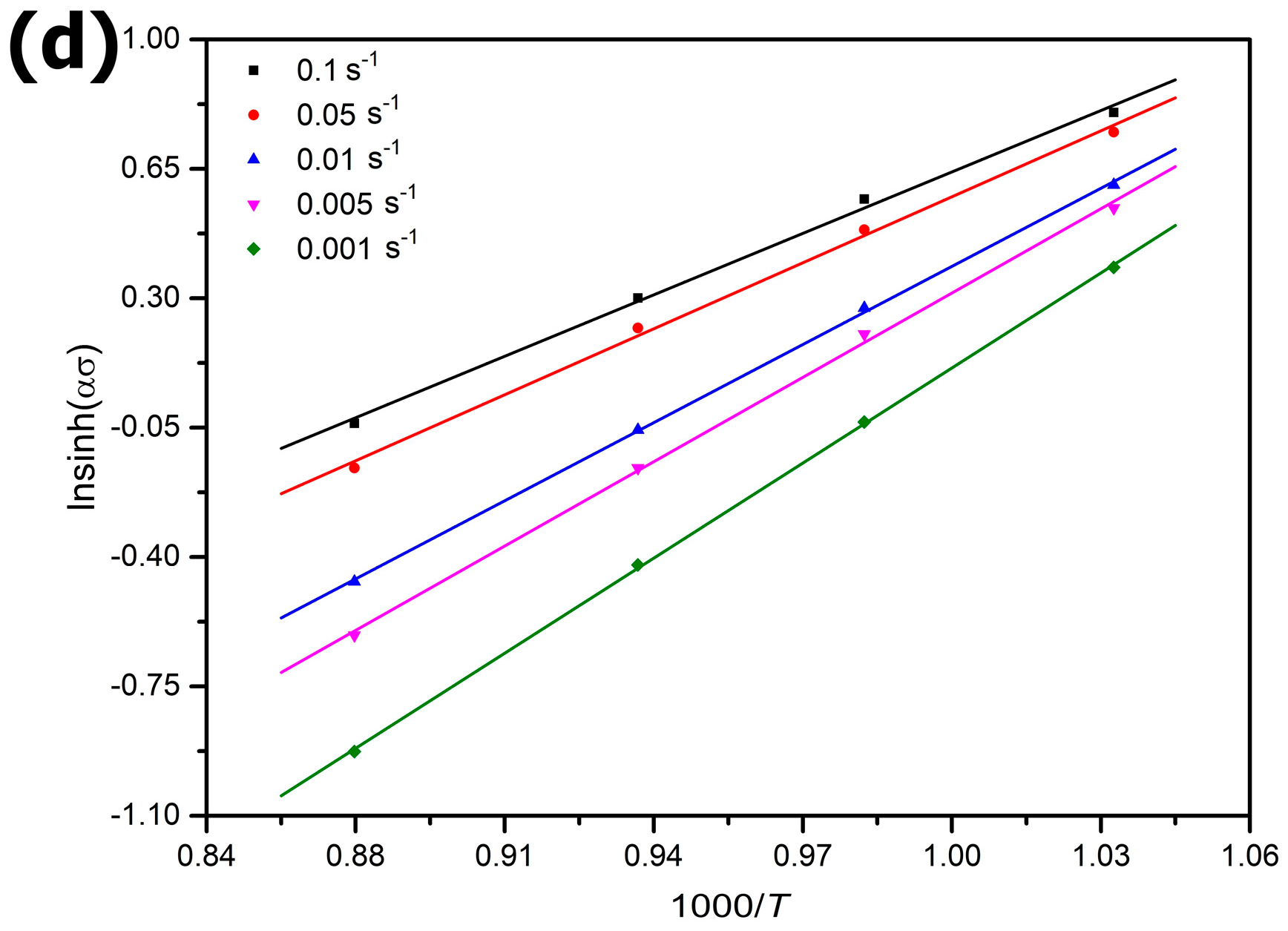
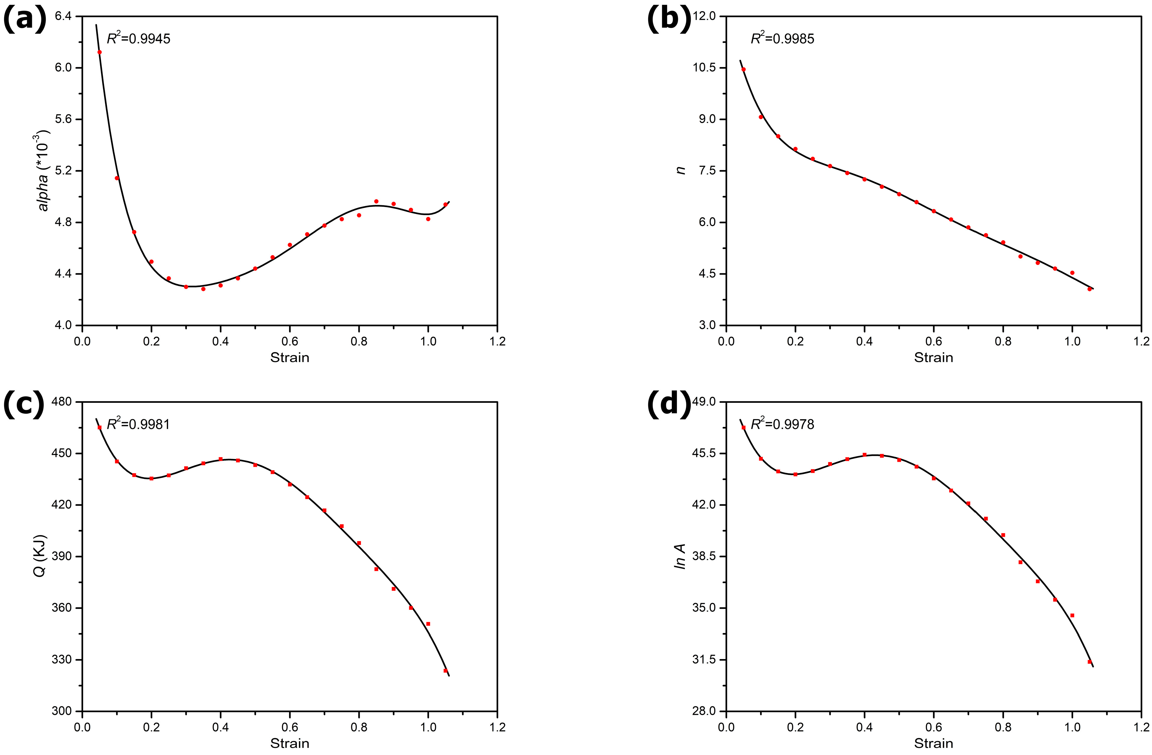
3.4. Strain–Compensated Arrhenius Model

The flow stress of metallic material during deformation is not only related to the chemical composition and microstructure, but also the deformation temperature, strain rate, and true strain. The hyperbolic-sine Arrhenius equation and Zener–Hollomon parameter (Z) were widely used to predict the flow stress and illustrate the deformation behavior in the past few decades [26,27,36], it can be written as follows:

$$\dot{\epsilon }=A{\left[\sin \mathrm{h}\left(\alpha \ast \sigma \right)\right]}^n\exp \left(-\frac{Q}{RT}\right)$$

(9)

$$Z=\dot{\epsilon }\exp \left(\frac{Q}{RT}\right)=A{\left[\sin \mathrm{h}\left(\alpha *\sigma \right)\right]}^n$$

(10)

where A, α, n, and Q are material dependent constants; $\dot{\epsilon }$ and σ have the same meaning with the MJC model; Q, R, and T denote the activation energy, the universe gas constant, and the absolute temperature, respectively.

The detailed procedures for solving the material constants also can be found elsewhere [26,27,31]. The calculation order of the constants or parameters related to the Arrhenius Model is as follows. $n^{\prime }$, which is the inverse of the slope of the fitting line $\ln \dot{\epsilon }~ \ln \sigma$ at each temperature. β, which is the inverse of the slope of the fitting line $\ln \dot{\epsilon } ~ \sigma$ at each temperature. α, $\alpha =\beta /n^{\prime }$. $n$, which is the inverse of the slope of the fitting line $\ln \left[\sinh \left(\alpha \sigma \right)\right] ~ \ln \dot{\epsilon }$ at each temperature. Q, which equals to the slope of the fitting line $\ln \left[\sinh \left(\alpha \sigma \right)\right]-1/T$ at each strain rate multiply n and R. The calculational process of peak stress at different temperature and strain rates is shown in Figure 8.

Based on the procedures mentioned above, the material constants of α, n, Q and lnA in the SCA equation can be obtained at strain from 0.05 to 1.05 with an interval of 0.05, and the results are shown in

Table 2. Material constants values in SCA model at different strains.

ε	α*10−3	n	Q (kJ)	lnA
0.05	6.12	10.46	465.16	47.26
0.1	5.14	9.07	445.36	45.14
0.15	4.73	8.51	437.43	44.28
0.2	4.50	8.14	435.42	44.08
0.25	4.37	7.85	437.26	44.30
0.3	4.30	7.64	441.43	44.79
0.35	4.28	7.44	444.24	45.12
0.4	4.31	7.25	446.79	45.42
0.45	4.37	7.04	445.95	45.34
0.5	4.44	6.82	443.28	45.06
0.55	4.53	6.59	439.12	44.60
0.6	4.63	6.33	431.94	43.81
0.65	4.71	6.09	424.58	42.98
0.7	4.78	5.86	416.86	42.11
0.75	4.83	5.63	407.69	41.08
0.8	4.86	5.42	397.85	39.96
0.85	4.96	5.01	382.68	38.11
0.9	4.94	4.82	371.17	36.82
0.95	4.90	4.66	360.07	35.56
1	4.83	4.53	350.78	34.50
1.05	4.94	4.06	323.69	31.37

and red dots in Figure 9. It can be seen the strain has a significant effect on the material constants. As to improve the accuracy of the Arrhenius Model, 6th order polynomial equations as shown in Equation (11) were used to demonstrate the relations between strain and the strain-dependent constants. The non-linear polynomial fitting curves and the square of the regression coefficients that correspond to α, n, Q, and lnA also can be found in Figure 9. Each square of the regression coefficient is close to 1, which indicates the proposed 6th order polynomial equations have a higher prediction accuracy and the parameters in Equation (11) are shown in

Table 3. Polynomial fitting parameters of α, n, Q, and lnA in SCA constitutive model.

	${\mathit{C}}_0$	${\mathit{C}}_1$	${\mathit{C}}_2$	${\mathit{C}}_3$	${\mathit{C}}_4$	${\mathit{C}}_5$	${\mathit{C}}_6$
α	0.008	−0.037	0.173	−0.425	0.583	−0.415	0.118
n	12.33	−47.96	211.45	−497.03	608.14	−373.45	90.92
Q	498.29	−848.11	3925.27	−7309.38	5351.70	−802.00	−469.89
lnA	50.80	−90.40	413.82	−745.30	495.57	−19.85	−70.71

.

$$Y\left(\epsilon \right)=C_0+C_1\epsilon +C_2{\epsilon }^2+C_3{\epsilon }^3+C_4{\epsilon }^4+C_5{\epsilon }^5+C_6{\epsilon }^6$$

(11)

The SCA constitutive equation related to Zener–Hollomon parameter can be rewritten in the following form, and the flow stress during compression can be predicted with the material constants α, n, Q, and A, which are a function of 6th order polynomial equations with the parameters in Table 3.

$$\sigma =\frac{1}{\alpha }\ln \left\{{\left[\frac{\dot{\epsilon }}{A}\exp \left(\frac{Q}{RT}\right)\right]}^{1/n}+{\left\{{\left[\frac{\dot{\epsilon }}{A}\exp \left(\frac{Q}{RT}\right)\right]}^{2/n}+1\right\}}^{1/2}\right\}$$

(12)

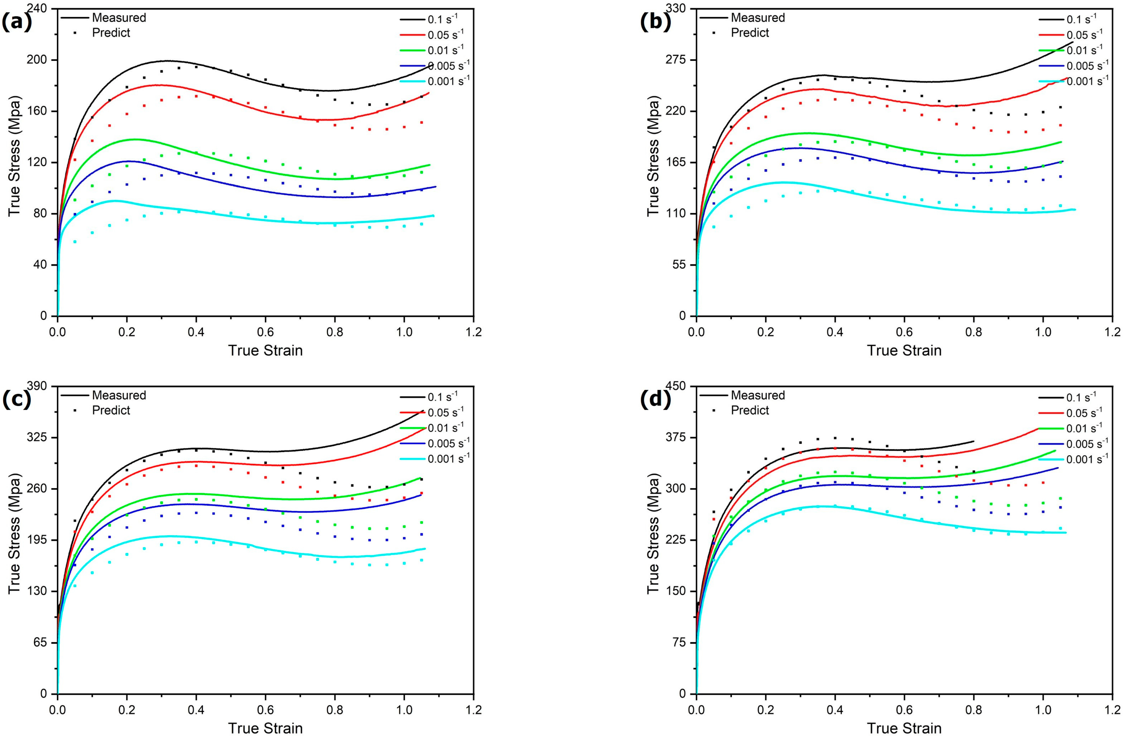
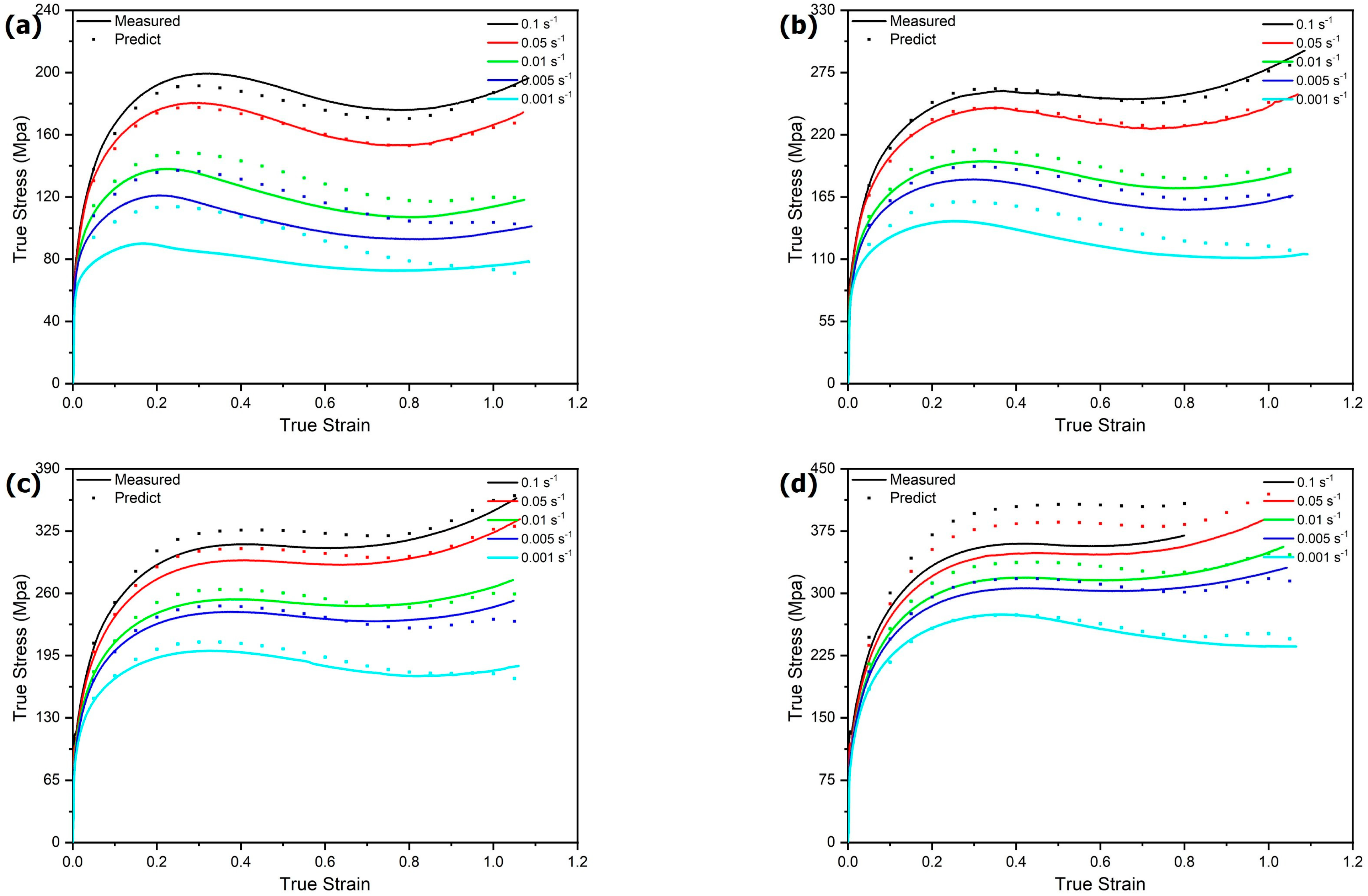
3.5. Evaluation of the Constitutive Models

Comparisons between the experimental and calculational flow stress using MJC and SCA models are shown in Figure 10 and Figure 11, respectively. The MJC model presents a good accuracy close to the reference conditions (0.001 s⁻¹ and 700 °C), the discrepancy between the predicted and measured stress values are negligible when the strain rate equal to 0.001 s⁻¹. As the compression temperature and strain rate increased from the reference conditions to a higher level, the discrepancy seems to expand. Moreover, when the true strain was larger than 0.6, the discrepancy was also gradually expanding with the increase in strain. The SCA model seems to have a relatively higher accuracy when the compression temperature is below Ac3 with a strain rate lower than 0.01 s⁻¹, and when it is higher than Ac3 with a strain rate larger than 0.01 s⁻¹. However, from the point of the shape of the predicted curves, the SCA model is much better than the MJC model.

The deviation of the calculational flow stress from the experimental curves was investigated quantitatively by using two parameters, the correlation coefficient (R) and the absolute average error (AARE), and their equations can be expressed as follows [13,16,17]:

$$R=\frac{{{\displaystyle \sum }}_{i=1}^N\left(E_i-\overline{E}\right)\left(P_i-\overline{P}\right)}{\sqrt{{{\displaystyle \sum }}_{i=1}^N{\left(E_i-\overline{E}\right)}^2{{\displaystyle \sum }}_{i=1}^N{\left(P_i-\overline{P}\right)}^2}}$$

(13)

$$AARE=\frac{1}{N}{\displaystyle \sum _{i=1}^N}\left|\frac{E_i-P_i}{E_i}\right|\ast 100$$

(14)

where $E_i$ is the experimental flow stress and $P_i$ is the calculational flow stress predicted using the above two models, $\overline{E}$ and $\overline{P}$ are the average of experimental and calculational flow stresses, respectively. N is the number of data (equal to 21) used in this study for a single true stress–strain curve. The R and AARE values under different compression temperatures and strain rates are shown in

Table 4. The R and AARE values of the MJC model and the SCA model at different compressive conditions.

Deformation Temperature (°C)	Strain Rate (s−1)	MJC Model		SCA Model
		R	AARE (%)	R	AARE (%)
870	0.001	0.19	7.36	0.86	18.93
	0.005	0.32	7.45	0.91	14.05
	0.01	0.45	6.94	0.93	9.18
	0.05	0.77	5.71	0.99	1.00
	0.1	0.86	4.33	0.98	2.92
800	0.001	0.57	6.45	0.97	12.10
	0.005	0.82	6.01	0.97	5.81
	0.01	0.88	6.25	0.99	4.87
	0.05	0.72	8.18	1.00	0.92
	0.1	0.52	8.09	0.99	1.23
750	0.001	0.93	4.89	0.95	3.53
	0.005	0.69	9.75	0.90	2.73
	0.01	0.59	8.71	0.93	2.82
	0.05	0.48	8.99	0.99	2.83
	0.1	0.45	8.46	0.99	3.71
700	0.001 *	0.98	1.49	0.97	2.10
	0.005	0.56	6.64	0.96	2.70
	0.01	0.49	7.34	0.96	3.57
	0.05	0.50	7.74	0.99	9.08
	0.1 #	0.83	5.21	1.00	11.61
All considered		0.97	6.82	0.99	5.71

* represent the reference test condition for the MJC model. ^# total strain is 0.8 for this test and 1.1 for the others.

. Generally, a higher value of R and lower value of AARE are usually considered as better parameters for prediction accuracy for the constitutive models. It is interesting that the R values in the MJC model, which are varied in a wide range from 0.19 to 0.98 at different conditions, but have a relatively higher value of 0.97 when all data were considered. The correlation coefficient reflects the degree of linear correlation between the calculational and experimental flow stress, the greater the absolute value of $R$ indicates the stronger the correlation. When the changing trend of the flow stress, with the increase in strain, is similar for the calculational and experimental values, the absolute value of R will increase correspondingly. The maximum value of R could reach is 1, which means there exists a linear relationship between the calculational and experimental values. Each R value in Table 4 that corresponds to a given compression condition can not represent the overall trend of flow stress data. The value of R depends on the stress–strain data that is selected, that is why the R value was much higher when all data were considered in the MJC model. Other researchers also mentioned that a higher R value does not always mean better accuracy of the model [13,17], because compared to the experimental curves, the calculational flow stress may deviate upward or downward. The unbiased AARE values can also be found in Table 4, and the values are 6.82% and 5.71% when all the stress–strain data were considered, which also indicates that the SCA model is more accurate. It should be noted that it is much more difficult to obtain the material dependent constants of the SCA constitutive model in terms of computational cost and complexity.

The correlation between the experimental and calculational flow stress which is predicted using the MJC and SCA models is shown in Figure 12. The black line with a slope of 1 indicates the exactly suitable position between the experimental and calculational values. It can be seen that the MJC model has many data points that deviated from the black line, while the SCA model has fewer. Moreover, the degree of deviation is relatively small when the flow stress is lower than about 200 Mpa for the MJC model and 325 Mpa for the SCA model, which indicates that the two proposed models are suitable to predict the flow stress at higher temperatures and lower strain rates, but for higher flow stress usually obtained at lower temperatures or higher strain rates, the SCA models seem much better.

4. Summary

Based on the above study, some conclusions could be drawn as follows:

(1) The true stress–strain curve is much more like a sine curve when the compression temperature is above Ac3 or the strain rate is small enough, because the dynamic softening effect is more significant at a higher temperature and a lower strain rate. The softening effect is not obvious when the temperature is below Ac3 with a strain rate that exceeds 0.005 s⁻¹.

(2) The MJC model has a good accuracy close to the reference condition (0.001 s⁻¹ and 700 °C). With the increase in compression temperature or increase in strain rate, the discrepancy between the MJC predicted flow stress and the measured flow stress expanded gradually, especially when the true strain larger than 0.6.

(3) The correlation coefficient R reflects the degree of linear correlation between the calculational and experimental flow stress under different conditions. The value of R depends on the stress–strain data that are selected, a higher R value does not imply a better prediction accuracy. The unbiased AARE values were 6.82 and 5.71 for MJC model and SCA model, respectively, which implied the SCA model has higher accuracy than the MJC model.

(4) The MJC and SCA models are suitable to predict the thermomechanical behavior of 5CrNiMoV steel when the flow stress lower than 200 Mpa. For a higher flow stress state, the SCA model is more preferred.

References

1. Huang, W.; Lei, L.; Fang, G. Microstructure evolution of hot work tool steel 5CrNiMoV throughout heating, deformation and quenching. Mater. Charact. 2020, 163, 110307. [Google Scholar] [CrossRef]
2. Birol, Y. Response to thermal cycling of duplex-coated hot work tool steels at elevated temperatures. Mater. Sci. Eng. A 2011, 528, 8402–8409. [Google Scholar] [CrossRef]
3. Lu, H.F.; Xue, K.N.; Xu, X.; Luo, K.Y.; Xing, F.; Yao, J.H.; Lu, J.Z. Effects of laser shock peening on microstructural evolution and wear property of laser hybrid remanufactured Ni25/Fe104 coating on H13 tool steel. J. Mater. Process. Technol. 2021, 291, 117016. [Google Scholar] [CrossRef]
4. Kheirandish, S.; Noorian, A. Effect of niobium on microstructure of cast AISI H13 hot work tool steel. J. Iron Steel Res. Int. 2008, 15, 61–66. [Google Scholar] [CrossRef]
5. Lee, S.J.; Lee, Y.K. Finite element simulation of quench distortion in a low-alloy steel incorporating transformation kinetics. Acta Mater. 2008, 56, 1482–1490. [Google Scholar] [CrossRef]
6. Katoch, S.; Sehgal, R.; Singh, V.; Gupta, M.K.; Mia, M.; Pruncu, C.I. Improvement of tribological behavior of H-13 steel by optimizing the cryogenic-treatment process using evolutionary algorithms. Tribol. Int. 2019, 140, 105895. [Google Scholar] [CrossRef]
7. Kweon, H.D.; Kim, J.W.; Song, O.; Oh, D. Determination of true stress-strain curve of type 304 and 316 stainless steels using a typical tensile test and finite element analysis. Nucl. Eng. Technol. 2021, 53, 647–656. [Google Scholar] [CrossRef]
8. Arrayago, I.; Real, E.; Gardner, L. Description of stress-strain curves for stainless steel alloys. Mater. Des. 2015, 87, 540–552. [Google Scholar] [CrossRef]
9. Sani, S.A.; Arabi, H.; Ebrahimi, G.R. Hot deformation behavior and DRX mechanism in a γ-γ/cobalt-based superalloy. Mater. Sci. Eng. A 2019, 764, 138165. [Google Scholar] [CrossRef]
10. Zhao, X.; Zang, X.; Wang, Q.; Park, J.; Yang, Q. Numerical simulation of the stress-strain curve and the stress and strain distributions of the titanium-duplex alloy. Rare Met. 2008, 27, 463–467. [Google Scholar] [CrossRef]
11. He, X.; Yu, Z.; Lai, X. A method to predict flow stress considering dynamic recrystallization during hot deformation. Comput. Mater. Sci. 2008, 44, 760–764. [Google Scholar] [CrossRef]
12. Gupta, A.K.; Anirudh, V.K.; Singh, S.K. Constitutive models to predict flow stress in austenitic stainless steel 316 at elevated temperatures. Mater. Des. 2013, 43, 410–418. [Google Scholar] [CrossRef]
13. Sabokpa, O.; Zarei-Hanzaki, A.; Abedi, H.R.; Haghdadi, N. Artificial neural network modeling to predict the high temperature flow behavior of an AZ81 magnesium alloy. Mater. Des. 2012, 39, 390–396. [Google Scholar] [CrossRef]
14. Srinivasu, G.; Rao, R.N.; Nandy, T.K. Finite element modeling of stress-strain curve and the stress and strain distributions of the Ti-10V-4.5Fe-3Al alloy. In Proceedings of the International Conference on Computational Techniques and Artificial Intelligence, Pattaya, Thailand, 7–8 October 2011; pp. 217–221. [Google Scholar]
15. Callister, W.D. Materials Science and Engineering an Introduction; John Wiley & Sons, Inc. Press: Hoboken, NJ, USA, 2007. [Google Scholar]
16. He, A.; Xie, G.; Zhang, H.; Wang, X. A comparative study on Johnson–Cook, Modified Johnson–Cook and Arrhenius-type constitutive models to predict the high temperature flow stress in 20CrMo alloy steel. Mater. Des. 2013, 52, 677–685. [Google Scholar] [CrossRef]
17. Zhao, Y.; Sun, J.; Li, J.; Yan, Y.; Wang, P. A comparative study on Johnson–Cook and Modified Johnson–Cook constitutive material model to predict the dynamic behavior laser additive manufacturing FeCr alloy. J. Alloys Comp. 2017, 723, 179–187. [Google Scholar] [CrossRef]
18. He, J.; Chen, F.; Wang, B.; Zhu, L.B. A Modified Johnson–Cook Model for 10%Cr steel at elevated temperatures and a wide range of strain rates. Mater. Sci. Eng. A 2018, 715, 1–9. [Google Scholar] [CrossRef]
19. Samantaray, D.; Mandal, S.; Borah, U.; Bhaduri, A.K.; Sivaprasad, P.V. A thermo-viscoplastic constitutive model to predict elevated-temperature flow behaviour in a titanium-modified austenitic stainless steel. Mater. Sci. Eng. A 2009, 562, 1–6. [Google Scholar] [CrossRef]
20. Raut, N.; Shinde, S.; Yakkundi, V. Determination of Johnson Cook parameters for Ti-6Al-4V Grade 5 experimentally by using three different methods. Mater. Today Proc. 2021, 44, 1653–1658. [Google Scholar] [CrossRef]
21. Zhu, S.; Liu, J.; Deng, X. Modification of strain rate strengthening coefficient for Johnson–Cook constitutive model of Ti6Al4V alloy. Mater. Today Commun. 2021, 26, 102016. [Google Scholar] [CrossRef]
22. Bobbili, R.; Madhu, V. A Modified Johnson–Cook Model for FeCoNiCr high entropy alloy over a wide range of strain rates. Mater. Lett. 2018, 218, 103–105. [Google Scholar] [CrossRef]
23. Tan, J.Q.; Zhan, M.; Liu, S.; Huang, T.; Guo, J.; Yang, H. A Modified Johnson–Cook Model for tensile flow behaviors of 7050-T7451 aluminum alloy at high strain rates. Mater. Sci. Eng. A 2015, 631, 214–219. [Google Scholar] [CrossRef]
24. Niu, L.; Cao, M.; Liang, Z.; Han, B.; Zhang, Q. A Modified Johnson–Cook Model considering strain softening of A356 alloy. Mater. Sci. Eng. A 2020, 789, 139612. [Google Scholar] [CrossRef]
25. Li, H.Y.; Li, Y.H.; Wang, X.F.; Liu, J.J.; Wu, Y. A comparative study on modified Johnson Cook, modified Zerilli-Armstrong and Arrhenius-type constitutive models to predict the hot deformation behavior in 28CrMnMoV steel. Mater. Des. 2013, 49, 493–501. [Google Scholar] [CrossRef]
26. Yang, P.; Liu, C.; Guo, Q.; Liu, Y. Variation of activation energy determined by a modified Arrhenius approach: Roles of dynamic recrystallization on the hot deformation of Ni-based superalloy. J. Mater. Sci. Technol. 2021, 72, 162–171. [Google Scholar] [CrossRef]
27. Ramana, A.V.; Balasundar, I.; Davidson, M.J.; Balamuralikrishnan, R.; Raghu, T. Constitutive modelling of a new high-strength low-alloy steel using modified Zerilli-Armstrong and Arrhenius Model. Trans. Indian Inst. Met. 2019, 72, 2869–2876. [Google Scholar] [CrossRef]
28. Lin, Y.C.; Chen, X.M. A combined Johnson–Cook and Zerilli-Armstrong model for hot compressed typical high-strength alloy steel. Comput. Mater. Sci. 2010, 49, 628–633. [Google Scholar] [CrossRef]
29. Lin, Y.C.; Chen, X.M.; Liu, G. A Modified Johnson–Cook Model for tensile behaviors of typical high-strength alloy steel. Mater. Sci. Eng. A 2010, 527, 6980–6986. [Google Scholar] [CrossRef]
30. Zhang, D.N.; Shangguan, Q.Q.; Xie, C.J.; Liu, F. A Modified Johnson–Cook Model of dynamic tensile behaviors for 7075-T6 aluminum alloy. J. Alloys Compd. 2015, 619, 186–194. [Google Scholar] [CrossRef]
31. Ashtiani, H.R.R.; Parsa, M.H.; Bisadi, H. Constitutive equations for elevated temperature flow behavior of commercial purity aluminum. Mater. Sci. Eng. A 2012, 545, 61–67. [Google Scholar] [CrossRef]
32. Xiao, D.; Peng, X.; Liang, X.; Deng, Y.; Xu, G.; Yin, Z. Research on constitutive models and hot workability of as-homogenized Al-Zn-Mg-Cu alloy during isothermal compression. Met. Mater. Int. 2017, 23, 591–602. [Google Scholar]
33. Chen, X.; Liao, Q.; Niu, Y.; Jia, W.; Le, Q.; Cheng, C.; Yu, F.; Cui, J. A constitutive relation of AZ80 magnesium alloy during hot deformation based on Arrhenius and Johnson–Cook model. J. Mater. Res. Technol. 2019, 8, 1859–1869. [Google Scholar] [CrossRef]
34. Hou, Q.Y.; Wang, J.T. A Modified Johnson–Cook constitutive model for Mg-Gd-Y alloy extended to a wide range of temperatures. Comput. Mater. Sci. 2010, 50, 147–152. [Google Scholar] [CrossRef]
35. Mirza1, F.A.; Chen, D.; Li, D.; Zeng, X. A Modified Johnson–Cook constitutive relationship for a rare-earth containing magnesium alloy. J. Rare Earths 2013, 31, 1202–1207. [Google Scholar] [CrossRef]
36. Liu, Y.; Li, M.; Ren, X.; Xiao, Z.; Zhang, X.; Huang, Y. Flow stress prediction of Hastelloy C-276 alloy using modified Zerilli-Armstrong, Johnson–Cook and Arrhenius-type constitutive models. Trans. Nonferrous Met. Soc. China 2020, 30, 3031–3042. [Google Scholar] [CrossRef]
37. Wang, X.; Huang, C.; Zou, B.; Liu, H.; Zhu, H.; Wang, J. Dynamic behavior and a Modified Johnson–Cook constitutive model of Inconel 718 at high strain rate and elevated temperature. Mater. Sci. Eng. A 2013, 580, 385–390. [Google Scholar] [CrossRef]
38. Instructions for First Use of a TA Instruments Dilatometer DIL805; TA Instruments: Hüllhorst, Germany, 2019.
39. Gleeble Users Training 2013 Gleeble Systems and Application; DSI Dynamic Systems Inc.: Austin, TX, USA, 2013.
40. Yang, Y.; Xu, D.; Cao, S.; Wu, S.; Zhu, Z.; Wang, H.; Li, L.; Xin, S.; Qu, L.; Huang, A. Effect of strain rate and temperature on the deformation behavior in a Ti-23.1Nb-2.0Zr-1.0O titanium alloy. J. Mater. Sci. Technol. 2021, 73, 52–60. [Google Scholar] [CrossRef]
41. Wang, Q.B.; Zhang, S.Z.; Zhang, C.J.; Zhang, W.G.; Yang, J.R.; Duo, D.; Zhu, D.D. The influence of the dynamic softening mechanism of α phase and γ phase on remnant lamellae during hot deformation. J. Alloys Comp. 2021, 872, 159514. [Google Scholar] [CrossRef]
42. Johnson, G.R.; Cook, W.H. A constitutive model and data for metals subjected to large strains, high strain rates and high temperatures. In Proceedings of the Seventh International Symposium on Ballistics, International Ballistics Committee, The Hague, The Netherlands, 19–21 April 1983; pp. 541–547. [Google Scholar]
Figure 1. (a) Schematic of compression tests for 5CrNiMoV steel, * denotes holding the specimen at 870 °C for 10 min, (b) the experimental setup and the upper right corner was the sample after compression.
Metals 12 01270 g001
Figure 2. True stress–strain curves of 5CrNiMoV steel at different strain rates. (a) 870 °C, (b) 800 °C, (c) 750 °C, and (d) 700 °C.
Metals 12 01270 g002
Figure 3. SEM morphologies of the 5CrNiMoV steel compressed at the strain rate of 0.05 s−1 and the temperature of: (a) 700 °C, (b) 750 °C, (c) 800 °C, and (d) 870 °C.
Metals 12 01270 g003
Figure 4. SEM morphologies of the 5CrNiMoV steel compressed at 870 °C and the strain rate of: (a) 0.001 s−1, (b) 0.005 s−1, (c) 0.01 s−1, and (d) 0.1 s−1.
Metals 12 01270 g004
Figure 5. Comparison between predicted and measured flow stress at 700 °C and the strain rate of 0.001 s−1 (referenced condition).
Metals 12 01270 g005
Figure 6. The relationship between σ / A 1 + B 1 ε + B 2 ε 2 + B 3 ε 3 ~   ln ε ˙ / ε r , used for obtaining C 1 in the MJC model.
Metals 12 01270 g006
Figure 7. The relationship between ln σ / A 1 + B 1 ε + B 2 ε 2 + B 3 ε 3 / 1 + C 1 ln ε ˙ * ~ T T r , used for obtaining the value of λ 1 + λ 2 ln ε ˙ * .
Metals 12 01270 g007
Figure 8. Linear fitting for obtaining the material dependent constants in the SCA constitutive equation. (a) n by fitting ln ε ˙   ~   ln σ , (b) β by fitting ln ε ˙   ~   σ , (c) n by fitting ln sinh α σ   ~   ln ε ˙ , (d) Q by fitting ln sinh α σ   ~   1000 / T .
Metals 12 01270 g008aMetals 12 01270 g008b
Figure 9. Non-linear polynomial fitting for obtaining the strain-dependent constants. (a) α, (b) n, (c) Q, and (d) lnA.
Metals 12 01270 g009
Figure 10. Comparison of flow stresses between MJC constitutive equation and compression tests at different strain rates. (a) 870 °C, (b) 800 °C, (c) 750 °C, and (d) 700 °C.
Metals 12 01270 g010
Figure 11. Comparison of flow stresses between SCA constitutive equation and compression tests at different strain rates. (a) 870 °C, (b) 800 °C, (c) 750 °C, and (d) 700 °C.
Metals 12 01270 g011
Figure 12. Correlation between the experimental and calculational flow stress. (a) MJC model, and (b) SCA model.
Metals 12 01270 g012