
The Isolated Austenite Forming during High-Temperature Cooling and Its Influence on Pitting Corrosion Resistance in S32750 Duplex Stainless Steel

 ,
,
Abstract
:1. Introduction
2. Material and Methods
3. Results
4. Discussion
4.1. Precipitation Mechanism of Isolated Austenite
4.1.1. Solution Temperature
4.1.2. Cooling Rates
4.2. Element Gradient and Pitting Corrosion Resistance
4.2.1. Element Contents
4.2.2. Specific Interfaces
5. Conclusions
- (1)
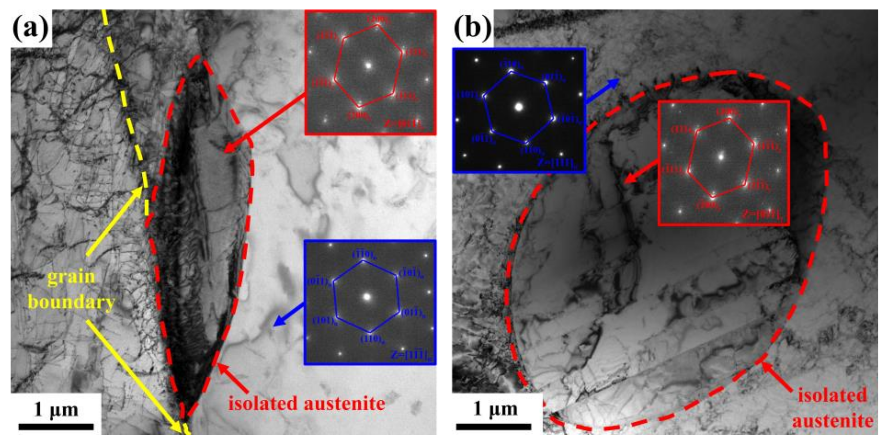
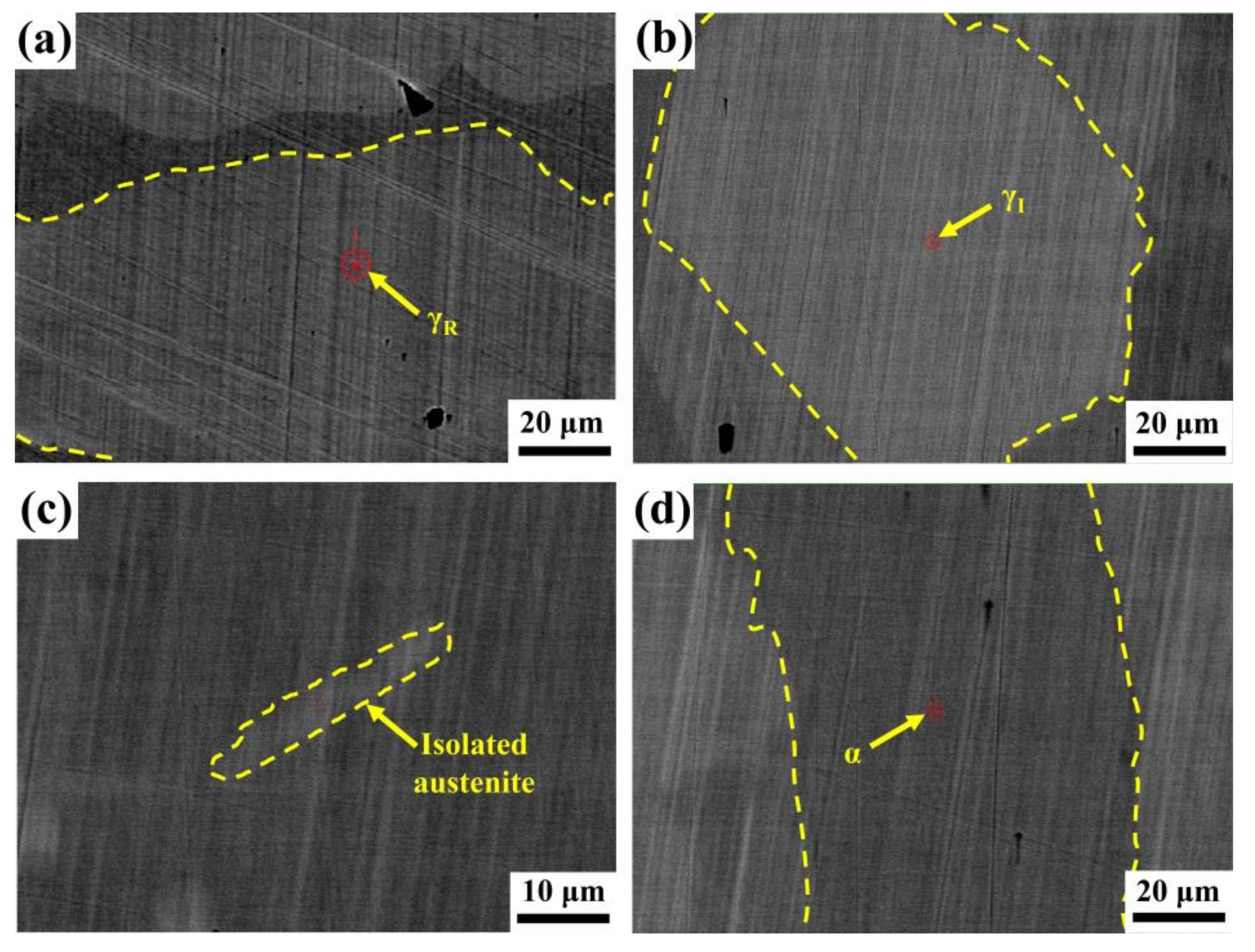
- Isolated austenite can be considered to be the product of an uneven diffusion of elements during rapid cooling from high temperatures, which mainly nucleates at ferrite grain boundaries or as intragranular ferrite grains, and presents a K-S orientation relationship with ferrite. N element segregates in IA.
- (2)
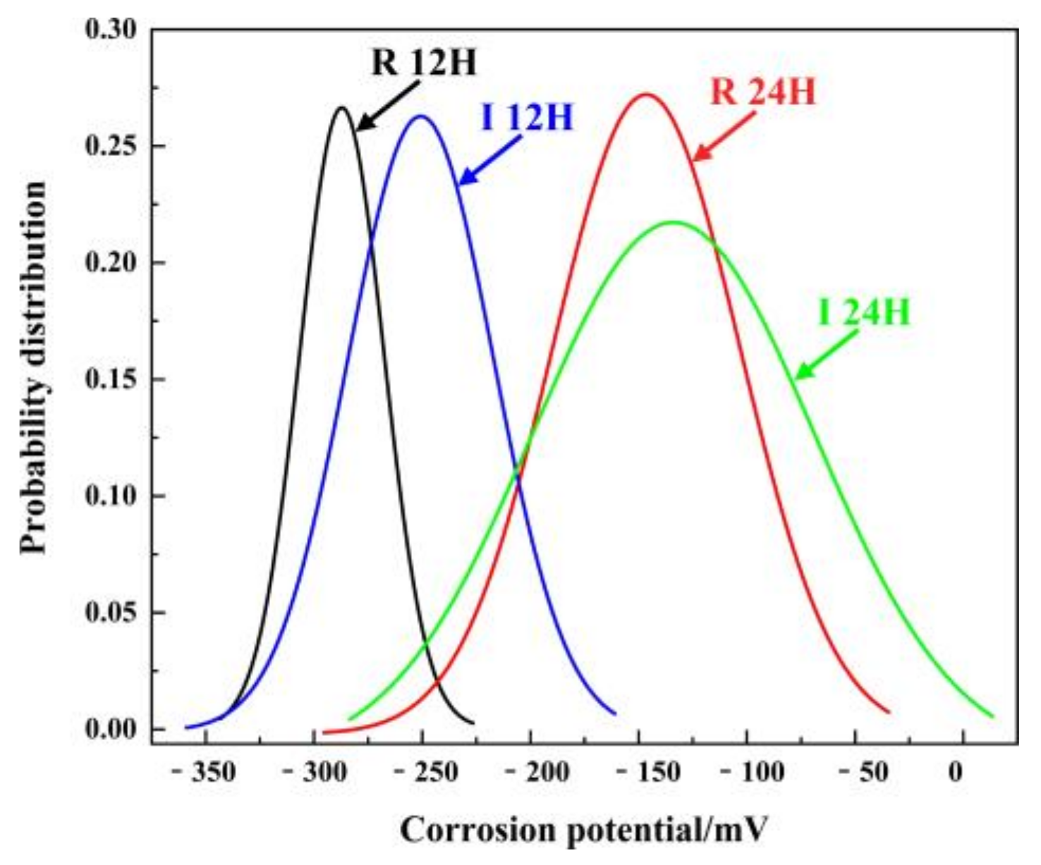
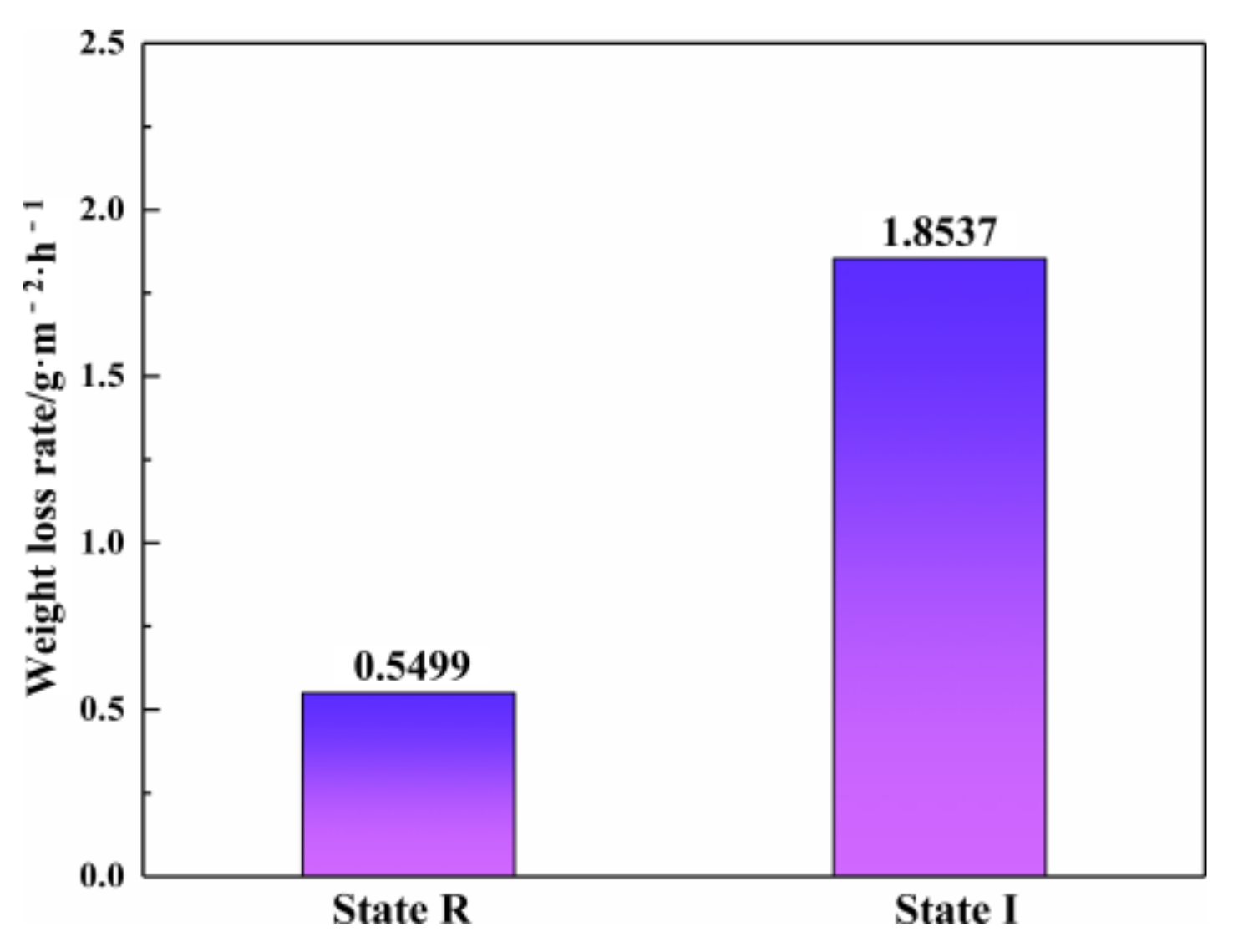
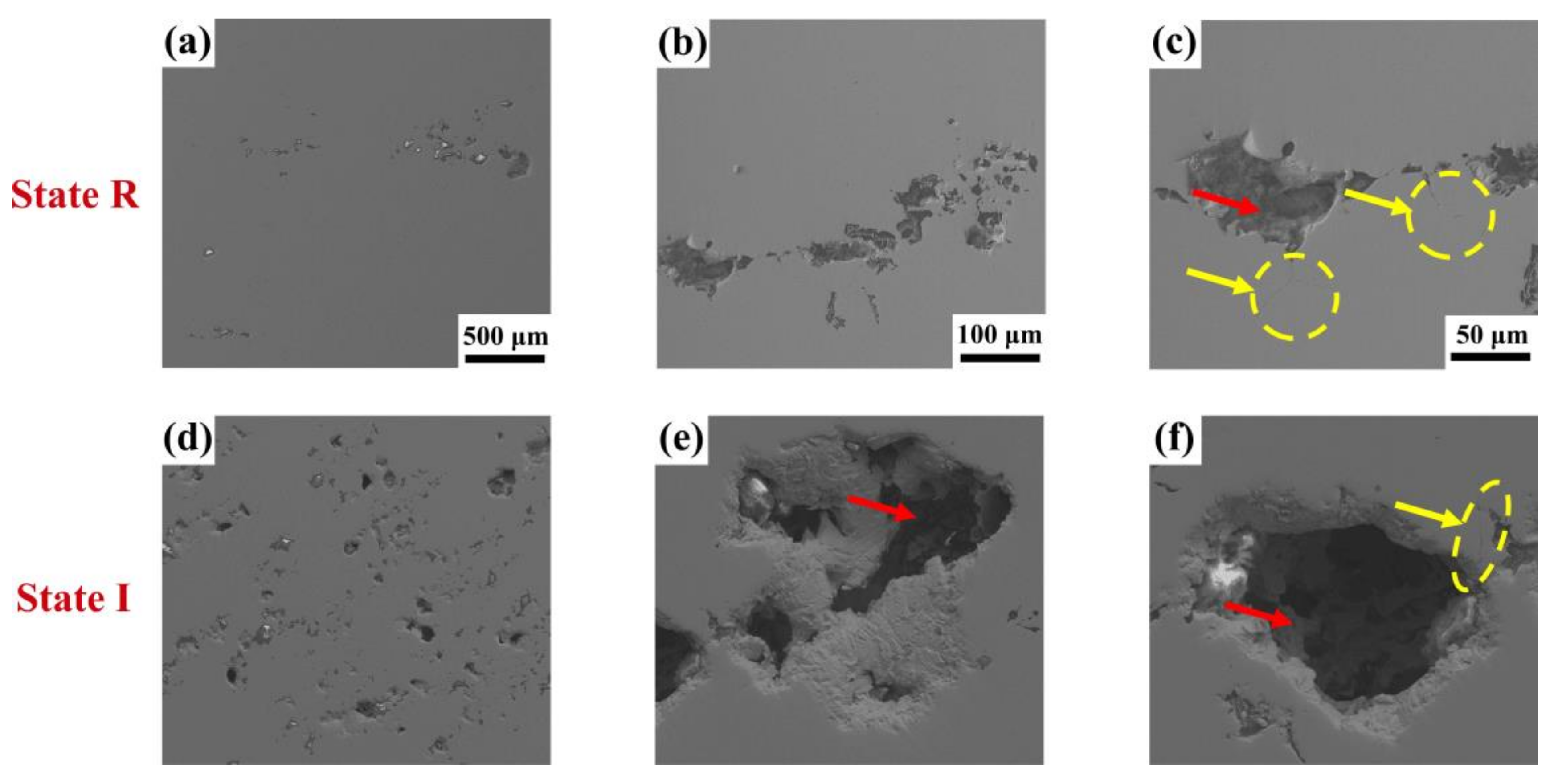
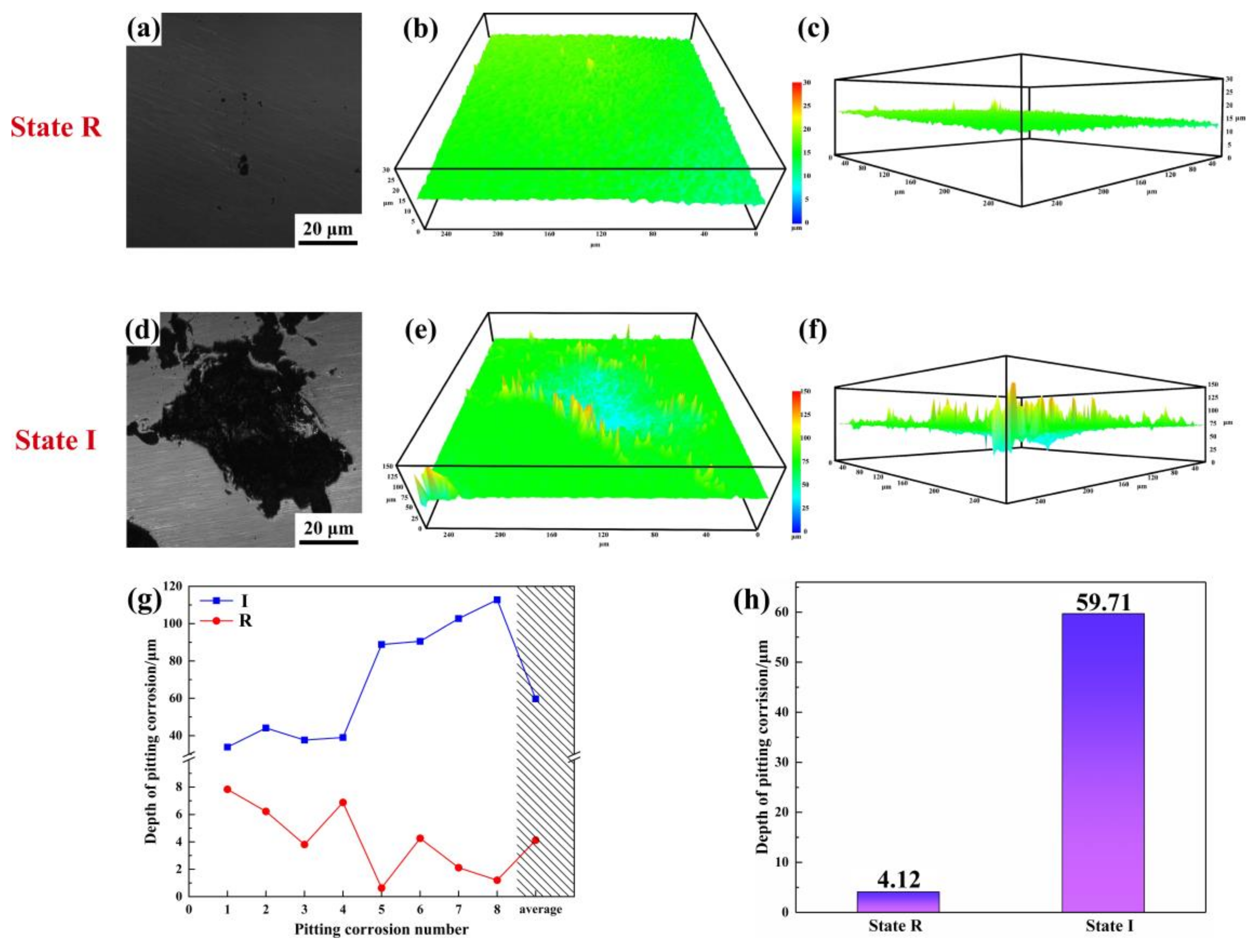
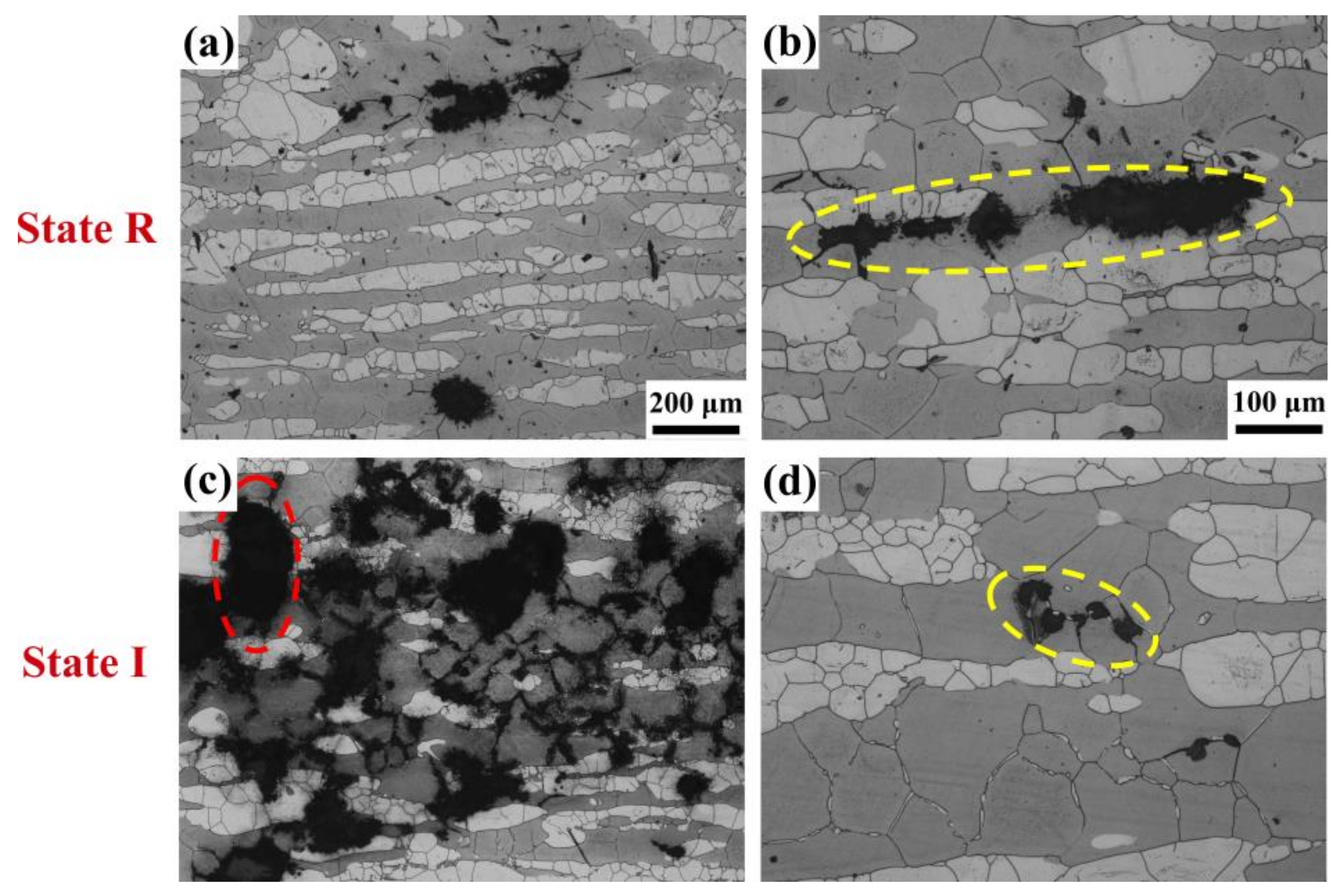
- With the precipitation of IA, the element concentration gradient is partially enhanced, leading to more frequent local corrosion. Pitting corrosion resistance significantly induces with the pitting depth increases by nearly 15 times. IA precipitated at ferrite grain boundaries furthers the deterioration of the pitting corrosion resistance.
- (3)
- The element redistribution phenomenon brought about by IA diminishes the PREN value of original austenite; thereby, the precedence order of pitting corrosion in DSS is: ferrite–austenite–IA.
Author Contributions
Funding
Data Availability Statement
Conflicts of Interest
References
- Wu, X.H.; Song, Z.G.; Liu, L.Z.; He, J.G.; Zheng, L. Effect of secondary austenite on fatigue behavior of S32750 super duplex stainless steel. Mater. Lett. 2022, 332, 132487. [Google Scholar] [CrossRef]
- Cojocaru, E.M.; Raducanu, D.; Nocivin, A.; Cinca, I.; Vintila, A.N.; Serban, N.; Angelescu, M.L.; Cojocaru, V.D. Influence of aging treatment on microstructure and tensile properties of a hot deformed UNS S32750 super duplex stainless steel (SDSS) alloy. Metals 2020, 10, 353. [Google Scholar] [CrossRef] [Green Version]
- Li, J.; Shen, W.; Lin, P.; Wang, F.; Yang, Z. Effect of solution treatment temperature on microstructural evolution, precipitation behavior, and comprehensive properties in UNS S32750 super duplex stainless steel. Metals 2020, 10, 1481. [Google Scholar] [CrossRef]
- Gennari, C.; Lago, M.; Bögre, B.; Meszaros, I.; Calliari, I.; Pezzato, L. Microstructural and corrosion properties of cold rolled laser welded UNS S32750 duplex stainless steel. Metals 2018, 8, 1074. [Google Scholar] [CrossRef] [Green Version]
- Helbert, V.S.; Nazarov, A.; Vucko, F.; Rioual, S.; Thierry, D. Hydrogen effect on the passivation and crevice corrosion initiation of AISI 304 using scanning kelvin probe. Corros. Sci. 2021, 182, 109225. [Google Scholar] [CrossRef]
- Nazarov, A.; Vucko, F.; Thierry, D. Scanning kelvin probe for detection of the hydrogen induced by atmospheric corrosion of ultra-high strength steel. Electrochim. Acta 2016, 216, 130–139. [Google Scholar] [CrossRef]
- Wu, X.H.; Song, Z.G.; Wang, B.S.; Wu, M.H.; Nai, Q.L.; Yao, L.; Feng, H.; Zheng, W.J. Morphologies of secondary austenite in 2507 duplex stainless steel after heat treatment. J. Iron Steel Res. Int. 2022, 29, 994–1003. [Google Scholar] [CrossRef]
- Haghdadi, N.; Cizek, P.; Hodgson, P.D.; Tari, V.; Rohrer, G.S.; Beladi, H. Effect of ferrite-to-austenite phase transformation path on the interface crystallographic character distributions in a duplex stainless steel. Acta Mater. 2017, 145, 196–209. [Google Scholar] [CrossRef]
- Du, J.; Zhang, W.Z.; Dai, F.Z.; Shi, Z.Z. Caution regarding ambiguities in similar expressions of orientation relationships. J. Appl. Crystallogr. 2016, 49, 40–46. [Google Scholar] [CrossRef]
- Tan, H.; Jiang, Y.; Deng, B.; Tao, S.; Xu, J.; Li, J. Effect of annealing temperature on the pitting corrosion resistance of super duplex stainless steel UNS S32750. Mater. Charact. 2009, 60, 1049–1054. [Google Scholar] [CrossRef]
- An, L.C.; Cao, J.; Wu, L.C.; Mao, H.H.; Yang, Y.T. Effects of Mo and Mn on pitting behavior of duplex stainless steel. J. Iron Steel Res. Int. 2016, 23, 1333–1341. [Google Scholar] [CrossRef]
- Ramirez, A.J.; Lippold, J.C.; Brandi, S.D. The relationship between chromium nitride and secondary austenite precipitation in duplex stainless steels. Metall. Mater. Trans. A 2003, 34, 1575–1597. [Google Scholar] [CrossRef]
- Jeon, S.H.; Kim, H.J.; Park, Y.S. Effects of inclusions on the precipitation of chi phases and intergranular corrosion resistance of hyper duplex stainless steel. Corros. Sci. 2014, 87, 1–5. [Google Scholar] [CrossRef]
- Chen, C.Y.; Yen, H.W.; Yang, J.R. Sympathetic nucleation of austenite in a Fe–22Cr–5Ni duplex stainless steel. Scr. Mater. 2007, 56, 673–676. [Google Scholar] [CrossRef]
- Shubina Helbert, V.; Nazarov, A.; Vucko, F.; Larché, N.; Thierry, D. Effect of Cathodic Polarisation Switch-Off on the Passivity and Stability to Crevice Corrosion of AISI 304L Stainless Steel. Materials 2021, 14, 2921. [Google Scholar] [CrossRef] [PubMed]
- Ma, C.Y.; Zhou, L.; Zhang, R.X.; Li, D.G.; Shu, F.Y.; Song, X.G.; Zhao, Y.Q. Enhancement in mechanical properties and corrosion resistance of 2507 duplex stainless steel via friction stir processing. J. Mater. Res. Technol. 2020, 9, 8296–8305. [Google Scholar] [CrossRef]
- Tarantseva, K.R. Models and methods of forecasting pitting corrosion. Prot. Met. Phys. Chem. Surf. 2010, 46, 139–147. [Google Scholar] [CrossRef]
- Guo, L.Q.; Bai, Y.; Xu, B.Z.; Pan, W.; Li, J.X.; Qiao, L.J. Effect of hydrogen on pitting susceptibility of 2507 duplex stainless steel. Corros. Sci. 2013, 70, 140–144. [Google Scholar] [CrossRef]


| Cr | Ni | Mo | N | Si | Mn | Fe | PREN | |
|---|---|---|---|---|---|---|---|---|
| γR | 24.93 ± 0.02 | 8.44 ± 0.02 | 2.96 ± 0.003 | 0.57 ± 0.012 | 0.31 ± 0.05 | 0.74 ± 0.01 | 62.11 ± 0.06 | 46.10 |
| γI | 24.63 ± 0.06 | 8.60 ± 0.01 | 2.94 ± 0.009 | 0.48 ± 0.002 | 0.18 ± 0.02 | 0.78 ± 0.02 | 60.65 ± 0.16 | 43.93 |
| IA | 23.91 ± 0.04 | 8.26 ± 0.03 | 2.98 ± 0.006 | 0.72 ± 0.01 | 0.20 ± 0.04 | 0.79 ± 0.01 | 60.56 ± 0.18 | 48.14 |
| α | 26.78 ± 0.03 | 5.54 ± 0.02 | 4.16 ± 0.02 | 0.00 ± 0.002 | 0.24 ± 0.03 | 0.73 ± 0.02 | 59.52 ± 0.09 | 40.51 |
| Potential Range/mV | ΔE/mV | xc/mV | w2 | |
|---|---|---|---|---|
| R 12 h | −342~−220 | 122 | −287.14 | (38.81)2 |
| I 12 h | −369~−155 | 214 | −250.68 | (67.21)2 |
| R 24 h | −302~−28 | 274 | −146.45 | (86.30)2 |
| I 24 h | −299~29 | 328 | −133.92 | (129.87)2 |
| Temperature/°C | 1200 | 1150 | 1100 |
| α | 0.049 | 0.034 | 0.023 |
| γ | 0.221 | 0.237 | 0.247 |
| Distribution coefficient (α/γ) | 0.22 | 0.14 | 0.09 |
| Temperature/°C | 1200 | 1150 | 1100 |
| Time/s | 10 | 9.60 | 8.80 |
| Elements | N | Cr | Mo | Ni | ||||
| Base metal | α-Fe | γ-Fe | α-Fe | γ-Fe | α-Fe | γ-Fe | α-Fe | γ-Fe |
| D0/cm2·s−1 | 0.0078 | 0.2 | 8.52 | 10.80 | 1.30 | 0.036 | 9.9 | 3 |
| Q/KJ·mol−1 | 79.10 | 151.00 | 250.80 | 291.80 | 229.00 | 240.00 | 259.20 | 314.00 |
| Temperature/°C | 1200 | 1150 | 1100 | 1200 | 1150 | 1100 | 1200 | 1150 | 1100 | 1200 | 1150 | 1100 |
| Elements | N | Cr | Ni | Mo | ||||||||
| γ | 36.4 | 28.7 | 21.8 | 0.85 | 0.55 | 0.34 | 0.18 | 0.11 | 0.07 | 0.41 | 0.28 | 0.19 |
| α | 135.4 | 118.4 | 100.4 | 4.04 | 2.76 | 1.80 | 3.09 | 2.09 | 1.34 | 3.84 | 2.71 | 1.82 |
Publisher’s Note: MDPI stays neutral with regard to jurisdictional claims in published maps and institutional affiliations. |
© 2022 by the authors. Licensee MDPI, Basel, Switzerland. This article is an open access article distributed under the terms and conditions of the Creative Commons Attribution (CC BY) license (https://creativecommons.org/licenses/by/4.0/).
Share and Cite
Wu, X.; Song, Z.; He, J.; Bao, Z.; Feng, H.; Zheng, W.; Zhu, Y. The Isolated Austenite Forming during High-Temperature Cooling and Its Influence on Pitting Corrosion Resistance in S32750 Duplex Stainless Steel. Metals 2022, 12, 1316. https://doi.org/10.3390/met12081316
Wu X, Song Z, He J, Bao Z, Feng H, Zheng W, Zhu Y. The Isolated Austenite Forming during High-Temperature Cooling and Its Influence on Pitting Corrosion Resistance in S32750 Duplex Stainless Steel. Metals. 2022; 12(8):1316. https://doi.org/10.3390/met12081316
Chicago/Turabian StyleWu, Xiaohan, Zhigang Song, Jianguo He, Zhiyi Bao, Han Feng, Wenjie Zheng, and Yuliang Zhu. 2022. "The Isolated Austenite Forming during High-Temperature Cooling and Its Influence on Pitting Corrosion Resistance in S32750 Duplex Stainless Steel" Metals 12, no. 8: 1316. https://doi.org/10.3390/met12081316
APA StyleWu, X., Song, Z., He, J., Bao, Z., Feng, H., Zheng, W., & Zhu, Y. (2022). The Isolated Austenite Forming during High-Temperature Cooling and Its Influence on Pitting Corrosion Resistance in S32750 Duplex Stainless Steel. Metals, 12(8), 1316. https://doi.org/10.3390/met12081316