
Fatigue Strength Estimation of Ductile Cast Irons Containing Solidification Defects

Department of Engineering & Architecture, University of Parma, Parco Area delle Scienze 181/A, 43124 Parma, Italy
Metals 2023, 13(1), 83; https://doi.org/10.3390/met13010083
Submission received: 25 November 2022
/
Revised: 14 December 2022
/
Accepted: 22 December 2022
/
Published: 29 December 2022
(This article belongs to the Special Issue Fatigue Behavior and Crack Mechanism of Metals and Alloys)
Abstract
:The goal of the present paper is to discuss the accuracy and reliability of a procedure for the fatigue strength estimation of defective metals by considering some experimental data available in the literature. In particular, the fatigue behaviour of three ductile cast irons (DCIs) containing solidification defects (i.e., micro-shrinkage porosity) is simulated through the above a procedure, based on the joined application of the -parameter model and the Carpinteri et al. multiaxial fatigue criterion. The fatigue strength of such DCIs subjected to both uniaxial (rotating bending or torsion) and biaxial (combined tension and torsion) cyclic loading is evaluated and compared with the experimental results.
1. Introduction
The presence of small defects is common in many real engineering components (for instance connecting rods, truck wheels, suspensions arms) made of casting metals such as high-strength steels [1,2,3,4,5], cast irons [6,7,8,9,10,11] and aluminium alloys [12,13]. Such defects, usually arising from the manufacturing process, are present in the form of non-metallic inclusions, slag inclusions, shrinkage porosities, gas pores, oxides and dross defects [14,15]. Moreover, these defects (also named solidification defects) can be encountered with different sizes (ranging from several µm to few mm) and shapes (spherical, elongated, or complex 3D geometry) and can be located both at the surface and in the bulk of the metallic components. Note that in the last years some optimisation procedures [16,17] have been developed in order to partially avoid the formation of solidification defects during the casting process, even if such defects cannot be completely removed.
Several studies conducted over the last forty years have demonstrated that solidification defects have a deleterious effect on mechanical properties under both monotonic and cyclic loading conditions [15]. As far as cyclic loadings are concerned, the solidification defects represent the preferential fatigue crack initiation sites and, consequently, metals containing such defects experience not only shorter fatigue life but also a larger scatter in fatigue strength with respect to their counterpart free from defects [13]. Since in real situations structural components can be subjected to cyclic loading, it is crucial to take into account the defect effects in the fatigue strength assessment in order to ensure a correct fatigue design and an appropriate in-service durability.
In such a context, three typical approaches for fatigue assessment of defective metals are available in the literature [18], and more precisely:
- -
- approach (a): the defects are treated as notches and the fatigue limit is calculated on the basis of the elastic stress concentration factor [19,20]. Note that, since the actual value of such a factor is difficult to be determined in presence of defects with an irregular shape, Mitchell [19] proposed to consider the defect equivalent to a hemispherical pit;
- -
- approach (b): the defects are considered as pre-existent cracks and the fatigue limit is determined by using the stress intensity factor concept [18,21]. The main drawback of this approach is related to the computation of the threshold stress intensity factor range, especially in presence of defects with a complex shape;
- -
According to the most relevant literature (see for instance the recent researches reported in Refs [24,25]), the -parameter model is the most employed approach in practical applications since only two quantities are required for the fatigue limit determination. Such quantities are the Vickers hardness (representative material parameter) and the defect size (representative geometrical parameter for defects), whereas no information regarding the shape of defects is required. Moreover, the model proposed by Murakami [22] and Yanase et al. [23] has proved to be in agreement with the experimental evidences that the size of the biggest defect is the controlling parameter of material fatigue strength [14].
Due to its unique features, the -parameter model has been implemented in several multiaxial fatigue criteria [1,14,24,25,26,27,28,29,30], providing satisfactory estimations in terms of fatigue strength of defective materials. For instance, Nadot and co-workers [14,26] analysed the accuracy of both the -parameter model and the Crossland multiaxial fatigue criterion in estimating the fatigue strength of steel specimens containing small defects with different shapes; subsequently, the Authors proposed a modified version of the Crossland criterion for defective materials. The -parameter model has been also implemented in the Dang Van fatigue criterion in order to simulate experimental tests performed on steel specimens with superficial and artificial spherical defects [27]. Moreover, Endo and Ishimoto [28] proposed a multiaxial fatigue criterion for the strength estimation of defective steels (with cylindrical defects) subjected to in-phase and out-of-phase cyclic loading. In particular, the fatigue limit under normal loading has been estimated by using the -parameter model by Murakami [22]. Recently, the research group of Araújo [1,25] has employed the -parameter model in order to calibrate the material constants of some well-known fatigue criteria available in the literature and based on the so-called critical plane approach (i.e., Fatemi-Socie, Smith-Watson-Topper, Findley and Modified Wöhler Curve Method criteria).
By following a similar approach of that proposed in Ref. [1], Vantadori and co-workers [29,30] have theoretically investigated the fatigue behaviour of defective metals (both a high-strength steel with non-metallic inclusions and a ductile cast iron with micro-shrinkage porosity) by employing a procedure based on the joined application of the -parameter model [22,23] and the multiaxial fatigue criterion by Carpinteri et al. [31,32,33,34,35,36]. More precisely, the fatigue limits under both normal and shear loading (i.e., criterion parameters) have been calculated by using the -parameter model, whereas the fatigue strength has been assessed by means of the Carpinteri et al. multiaxial fatigue criterion, based on the critical plane approach. It is important to point out that, since the defects were more than one in the analysed specimens, a defect content analysis has been performed through a statistical method deriving from the Extreme Value Theory (EVT) [37,38]. Moreover, such a statistical method has been also employed to determine an optimised return period for fatigue limit calculation.
It deserves to point out that the above defect content analysis can be easily performed by using machine learning techniques. As a matter of fact, the machine learning techniques have been recently employed to successfully predict the fatigue strength of both conventional and additive manufactured metals (see for instances Refs [39,40]).
By taking as starting point the procedure developed by Vantadori et al. [29,30], the goal of the present paper is to discuss the accuracy and reliability of such a procedure in simulating fatigue tests available in the literature and performed on three different Ductile Cast Irons (DCIs) containing solidification defects, in terms of micro-shrinkage porosity [6,41]. In particular, the fatigue strength of such DCIs subjected to both uniaxial (rotating bending or torsion) and biaxial (combined tension and torsion) cyclic loading is evaluated and compared with the experimental results.
The paper is structured as follows. Section 2 is dedicated to the description of the fundamentals of the present procedure for defective materials. The experimental campaign available in the literature is described in Section 3, whereas the defect content analysis together with the computation of the optimised return period are presented in Section 4. The discussion of the obtained results is reported in Section 5 and the main conclusions are summarised in Section 6.
2. Fundamentals of the Procedure for Fatigue Strength Estimation of Defective Metals
The procedure here employed to theoretically examine the fatigue behaviour of metals containing solidification defects is that proposed by Vantadori and co-workers [29,30]. Such a procedure implements: the -parameter model [22,23] and the Carpinteri et al. multiaxial fatigue criterion [31,32,33,34,35,36], as detailed in the following Sub-Sections. The flowchart of the above procedure can be found in Ref. [29].
Note that, the -parameter model is here employed since it takes into account the experimental evidences that the size of the biggest defect is the controlling parameter of fatigue limit determination. Moreover, the fatigue strength is assessed by using the Carpinteri et al. multiaxial fatigue criterion, being very accurate in simulating the fatigue behavior of several metallic components subjected to both uniaxial and multiaxial cyclic loading [31,32,33,34,35,36].
2.1. The -Parameter Model
The -parameter model, proposed in the past by Murakami [22] and Yanase et al. [23], allows to compute the fatigue limits under normal loading, , and shear loading, , of a defective material as functions of the values of and , which represent the square root of the expected maximum size of the defect related to normal and shear uniaxial cyclic loading, respectively.
In particular, according to Murakami proposal [22,37,38], the value of under normal cyclic loading is computed by using the following equation:
being the material Vickers hardness.
Under shear loading, the fatigue limit can be calculated by using the following relationship proposed by Yanase et al. [23]:
Note that, both the above equations are related to: (i) a number of loading cycles equal to and (ii) a defect just below the surface.
It is important to highlight that the values of and are usually predicted by using a statistical method, since it is virtually impossible to directly measure the area of the largest defect existing in a metallic component. More precisely, a statistical distribution of defects is derived by exploiting the EVT [37,38] and the so-called return periods related to both normal, , and shear, , uniaxial cyclic loading are obtained. Finally, the and values are computed on the basis of the values of and , respectively. More details regarding such a statistical method can be found in Refs [1,29,30].
2.2. The Carpinteri et al. Multiaxial Fatigue Criterion
The multiaxial fatigue criterion, proposed in the past by Carpinteri and co-workers, is based on the critical plane approach and can be employed for the fatigue strength assessment of metallic components subjected to cyclic loading with constant amplitude [31,32,33,34,35,36]. In particular, the orientation of the critical plane (that is, the verification plane) is assumed to be linked to the averaged directions of the principal stress axes and the fatigue strength evaluation is performed by employing the amplitude of an equivalent stress related to the critical plane.
The present criterion consists in the following main steps, to be performed at the verification material point:
- determination of the averaged directions of the principal stress axes by means of the averaged values of the principal Euler angles, obtained through an appropriate weight function;
- definition of the critical plane orientation, which is linked to the above averaged principal stress directions through an off-angle , defined as follows:
- computation of the normal, , and shear, , components of the stress vector related to the critical plane orientation;
- estimation of the fatigue endurance condition by equating an equivalent uniaxial stress amplitude, , to the normal fatigue limit, , that is
The criterion accuracy in the fatigue strength assessment can be evaluated by means of an error index, defined as follows:
3. Experimental Fatigue Data Examined
The procedure for fatigue strength estimation of defective metals presented in Section 2 is hereafter applied to a set of data available in the literature and related to infinite life fatigue tests [6,41]. In particular, both uniaxial (rotating bending or torsion) and biaxial (combined tension and torsion) fatigue tests are analysed.
The investigated materials were three DCIs, and more precisely:
- -
- a ferritic DCI with 14% graphite nodules in a white ferrite matrix, identified as EN-GJS-400-18, according to the European designation;
- -
- a ferritic/pearlitic DCI with a typical bulls-eye structure of 14% graphite nodules in a matrix of 46% ferrite and 40% dark pearlite, identified as EN-GJS-600-3 DCI;
- -
- a pearlitic DCI with 13% graphite nodules in a matrix of 62% pearlite and 25% ferrite, identified as EN-GJS-700-2 DCI.
The chemical compositions of such DCIs are reported in Table 1, whereas the mechanical properties are listed in Table 2. Note that, the present values of the Vickers hardness, HV, were measured by considering a load of 98.1 N.
The small cylindrical smooth specimens, made by turning and milling from DCI large sections, were characterised by a diameter of the gauge section equal to 10 mm. The geometrical sizes of the specimens are reported in the original work by Endo and Yanase [6].
A specimen surface finishing with an emery paper was performed and, subsequently, a surface layer of about 30 µm was removed by electro-polishing. Moreover, in order to avoid that the surface defects would grow further during the electro-polishing, specimen surface was refinished with alumina paste (up to a depth of about 10 µm) and, then, 1–2 µm of the surface layer were removed by a second electro-polishing.
Regarding uniaxial fatigue tests, a rotating bending testing machine of uniform moment type (operating speed equal to 57 Hz) was used, whereas torsional and biaxial tests were performed by means of an MTS servo-hydraulic testing machine with an operating speed ranging from 30 Hz to 45 Hz.
All the fatigue tests, performed under the condition of constant amplitude loading with a sinusoidal waveform, were characterised by a loading ratio, , equal to −1. The ratio of the applied shear stress amplitude to the applied normal stress amplitude, , was equal to: (rotating bending), (combined tension and torsion) and (torsion). The phase shift, , between tensile and torsional loading was either 0° or 90° for EN-GJS-400-18 and EN-GJS-700-2 DCIs, whereas only proportional biaxial loading was considered for EN-GJS-600-3 DCI. Note that, the run-out condition was assumed when a specimen survived more than cycles.
From the uniaxial fatigue data, the fully reversed normal fatigue limits were computed [42,43], and more precisely: for EN-GJS-400-18 DCI, for EN-GJS-600-3 DCI and for EN-GJS-700-2 DCI. Regarding the fatigue limits under fully reversed shear loading, no data are available in the original research works [6,41,42,43].
Finally, as far as the rotating bending tests are concerned, one specimen of each analysed DCI was employed for the analysis of the defects. In particular, the fracture surface, normal to the specimen longitudinal axis, was examined by using a Scanning Electron Microscope (SEM), characterised by an inspection area, , equal to 0.5 mm2. It was observed that the largest micro-shrinkage porosity was usually the preferential site for fatigue crack nucleation. Therefore, the largest defect inside was detected and the square root of such a defect area, , was measured by considering the area of the circumscribed circle. Then, the above operation was repeated 50 times on each fracture surface of the three DCIs being examined. At the end of the above procedure, the values of (with ) for each DCI were determined. Note that, as reported by the Authors in Refs [6,41], it was not possible to measure a micro-shrinkage porosity with a value of smaller than 25 µm, due to the limits of the SEM.
4. Defect Content Analysis and Return Period Optimisation
By using the experimental data in terms of [6,41], a defect content analysis (based on a statistical method deriving from the EVT [37,38]) together with an optimisation procedure of the return period are hereafter performed for each of the examined DCI. Note that, due to the lack of experimental data, the obtained results for normal uniaxial cyclic loading are extended to shear one. In other words, the value of is assumed to be equal to value, that is, .
Firstly, in order to identify the defect statistical distribution, the experimental values of are arranged in ascending order for each DCI analysed:
Then, for each DCI, a reduced variable, , is calculated as follows:
Such a reduced variable is plotted against values, obtaining the probability graph of the defect distribution for the three DCIs, as shown in Figure 1. Independently of the analysed material, it can be noted that the probability graphs have a linear trend and linear regressions of the above defect distributions can be obtained (see the red dashed lines in Figure 1). More precisely, such regressions are given by the following equations:
with:
where is the return period related to normal uniaxial cyclic loading.
According to Equation (9), value is a function of value, which in turn depends on the volumes considered in the defect content analysis. More precisely, the probability of finding larger defects increases within the volume. The value is, hence, defined as the ratio of two volumes, that is:
where is the prediction volume related to the specimen useful cross-section and is the standard inspection volume related to normal uniaxial cyclic loading. The volume is calculated by assuming that the inspection area is characterised by a given thickness, , and more precisely:
with:
According to the experimental data reported in Refs [6,41], the value of is equal to µm for EN-GJS-400-18 DCI, µm for EN-GJS-600-3 DCI and µm for EN-GJS-700-2 DCI; consequently, for equal to mm2 (as reported in Section 3), turns to be equal to mm3 for EN-GJS-400-18 DCI, mm3 for EN-GJS-600-3 DCI and mm3 for EN-GJS-700-2 DCI.
By following the optimisation procedure proposed in Refs [29,30], different values of the prediction volume, , are hereafter employed in order to define an optimised return period, , for the computation of and, hence, of the fatigue limits and for the three DCIs analysed. The considered values of together with the corresponding values (Equation (11)) are listed in Table 3, Table 4 and Table 5 for EN-GJS-400-18 DCI, EN-GJS-600-3 DCI and EN-GJS-700-2 DCI, respectively.
According to Table 3, Table 4 and Table 5, the first four values of are computed as a function of the volume of the specimen gauge section (length mm and diameter mm) [6,41], and more precisely:
- -
- mm3 is the volume of the specimen gauge section for which the return period is ;
- -
- mm3 is five times the volume of the specimen gauge section (i.e., ) for which the return period is ;
- -
- mm3 is ten times the volume of the specimen gauge section (i.e., ) for which the return period is ;
- -
- mm3 is fifty times the volume of the specimen gauge section (i.e., ) for which the return period is .
Moreover, also the typical volume of a crankshaft (that is, mm3) is considered and the corresponding return period is named (see Table 3, Table 4 and Table 5). Finally, represents a fictitious prediction volume obtained by considering the experimental fatigue limit of each DCI analysed (see the data reported in Section 3). More precisely, by employing instead of in Equation (1), the corresponding value is derived for each DCI and, then, the fictitious prediction volume is obtained from Equation (9) together with Equation (10). Finally, the corresponding return period (see Equation (11)) is indicated as in Table 3, Table 4 and Table 5.
Once the values are obtained, the values are derived from Equation (9) for the three DCIs examined. Then, by assuming that (that is, ), the fatigue limits and are computed by means of Equations (1) and (2), and the values are listed in Table 3, Table 4 and Table 5. Finally, for each pair (,), the Carpinteri et al. multiaxial fatigue criterion (Section 2.2) is applied and the mean value of the error index, , is deduced through Equation (6) (see Table 3, Table 4 and Table 5).
The values vs. the values are plotted in Figure 2 for each DCI; it can be observed that the above points are well interpolated by logarithmic curves, obtaining the following relationships:
For each DCI, an optimised value of the return period, , is obtained from the above equations by equating the mean value of the error index to zero (i.e., ), as reported in Table 3, Table 4 and Table 5. Then, by exploiting Equation (9), is equal to: µm for EN-GJS-400-18 DCI, µm for EN-GJS-600-3 DCI and µm for EN-GJS-700-2 DCI; the fatigue limits and at loading cycles are, hence, computed for the three DCI being examined (see Table 3, Table 4 and Table 5).
5. Discussion of the Results
By taking as starting point the fatigue limits obtained at the end of the optimisation procedure of Section 4, the fatigue strength of the three DCIs containing solidification defects is evaluated by means of the Carpinteri et al. multiaxial fatigue criterion. In particular, the fatigue endurance condition of Equation (5) is represented by the against plot, reported in Figure 3, Figure 4 and Figure 5. For each DCI, the ellipse with semi-axis equal to and (solid line in Figure 3, Figure 4 and Figure 5) represents Equation (5); in the above Figures, the dashed and dot-dashed lines are the error bands equal to and , respectively. Moreover, the points correspond to the analysed fatigue data, being the full and empty symbols, respectively, the experimental failures and run-outs. Note that, if the above points lie out of the ellipse, the present procedure allows to predict fatigue failures; on the other hand, run-out conditions are estimated when such points are inside the elliptical domain.
From Figure 3, Figure 4 and Figure 5, it can be observed that the present procedure is in general able to correctly predict both the experimental failures and run-outs, independently of the loading condition (that is, uniaxial and biaxial loading). In particular, for EN-GJS-400-18 DCI (see Figure 3), the following remarks can be made:
- -
- for uniaxial fatigue tests (i.e., and ), the above procedure is able to correctly estimate the fatigue failures (being all the full symbols outside the ellipse), whereas the experimental run-out conditions are not capture, with the exception of one data relating to torsion. However, the empty symbols lie on or very close to the failure curve (within the error band equal to ), thus representing a condition of incipient failure;
- -
- for proportional biaxial fatigue tests (i.e., with ), all the experimental failures and one of the two run-outs are perfectly predicted by means of the present procedure;
- -
- for non-proportional biaxial fatigue tests (i.e., with ), all the empty symbols are inside the elliptical domain, in agreement with the experimental observations. On the other hand, two of the three experimental failures are not capture by means of the present procedure, falling the results into the error band equal to .
From Figure 4 related to EN-GJS-600-3 DCI, it can be observed that:
- -
- for rotating bending fatigue tests (i.e., ), the fatigue failure conditions are perfectly estimated, whereas incipient failure conditions (i.e., the corresponding points lie very close to the failure curve) are obtained, even if run-outs were observed;
- -
- for torsion fatigue tests (i.e., ), the present procedure allows to correctly estimate the experimental run-out and one of the two experimental fatigue failure, while for the other it is possible to predict an incipient failure condition;
- -
- for proportional biaxial fatigue tests (i.e., with ), experimental run-outs are correctly represent by the empty symbols falling inside the elliptical domain; regarding fatigue failures, only one is perfectly predicted by means of the present procedure, whereas incipient failure conditions are achieved for the other two.
As far as EN-GJS-700-2 DCI is concerned (Figure 5), it can be pointed out that:
- -
- for rotating bending fatigue tests (i.e., ), the full symbols falling outside the elliptical domain correctly represent experimental failures, whereas the empty symbols should be located inside the ellipse, since run-outs were experimentally observed. However, such points lie very close to the failure curve (inside the error band equal to ), and, consequently, the procedure allows to estimate conditions of incipient failure;
- -
- for torsion fatigue tests (i.e., ), the experimental failure and run-out conditions are perfectly predicted by means of the present procedure;
- -
- for proportional biaxial fatigue tests (i.e., with ), all the full symbols are outside the elliptical domain, in agreement with the experimental outcomes. An incipient failure instead of a run-out is predicted, since the empty symbol is outside the ellipse, but very close to it;
- -
- for non-proportional biaxial fatigue tests (i.e., with ), the present procedure allows to correctly capture the run-outs but not the fatigue failures, even if the full symbols lie inside the error band equal to .
Finally, the effectiveness of the present procedure in estimating fatigue strength of defective DCIs can be evaluated from Figure 6, Figure 7 and Figure 8. As a matter of fact, by considering only the experimental data related to fatigue failures, the results in terms of equivalent uniaxial stress amplitude, , are plotted together with the fatigue limit of each DCI (see Table 3, Table 4 and Table 5), represented by a black solid line in the above Figures. Moreover, the experimental fatigue limits under fully reversed normal stress, , (reported in Section 3) are also depicted with red dashed lines in Figure 6, Figure 7 and Figure 8 for the materials being analysed.
It can be observed that the use of in the fatigue endurance condition of the present procedure (see Equation (5)) provides more conservative results with respect to those obtained when the experimental fatigue limit is employed, and this holds true for all the three DCIs. More precisely, for EN-GJS-400-18 DCI (Figure 6), and of the results are conservative when and are, respectively, used in the fatigue endurance condition. Regarding EN-GJS-600-3 DCI (Figure 7), and of conservative estimations are achieved if and are, respectively, employed. Finally, for EN-GJS-700-2 DCI (Figure 8), the present fatigue endurance condition in terms of provides of conservative results, whereas only is obtained by employing .
6. Conclusions
In the present paper, the accuracy and reliability of a procedure for fatigue strength estimation of defective metals have been discussed by considering some experimental data available in the literature. In particular, the fatigue behaviour of three DCIs containing solidification defects (i.e., micro-shrinkage porosity) has been simulated through a procedure based on the joined application of the -parameter model and the Carpinteri et al. multiaxial fatigue criterion.
More precisely, by taking as starting point the experimental data of each DCI, a defect content analysis has been performed by means of a statistical method deriving from the EVT. Subsequently, the above statistical method has been also employed to determine an optimised return period; by using such a return period, the fatigue limits under normal and shear loadings have been computed according to the -parameter model. Finally, for each DCI, the fatigue strength has been evaluated by considering the above fatigue limits in the Carpinteri et al. multiaxial fatigue criterion.
By means of the present procedure, an accurate evaluation of the fatigue endurance condition is achieved for the three defective DCIs here examined. In particular, such a procedure is in general able to correctly predict both fatigue failure and run-out conditions experimentally observed. Moreover, the use of the fatigue limit in the fatigue endurance condition of the present procedure provides more conservative results with respect to those obtained when the experimental fatigue limit is employed, and this holds true for all the three DCIs.
The obtained results demonstrate that it is crucial to take into account the influence of solidification defects on the fatigue strength assessment in order to avoid too non-conservative estimations, which are not in favour of safety. Therefore, the present procedure can be regarded as a powerful tool suitable for the fatigue design of real metallic components.
Funding
This research received no external funding.
Informed Consent Statement
Not applicable.
Conflicts of Interest
The author declares no conflict of interest.
Nomenclature
| square root of the expected maximum size of the defect under normal cyclic loading | |
| square root of the expected maximum size of the defect under shear cyclic loading | |
| amplitude of the shear stress component on the critical plane | |
| gauge section diameter | |
| thickness associated to the inspection area under normal cyclic loading | |
| Vickers hardness | |
| error index | |
| gauge length | |
| amplitude of the normal stress component perpendicular to the critical plane | |
| equivalent normal stress amplitude | |
| mean value of the normal stress component perpendicular to the critical plane | |
| loading ratio | |
| inspection area | |
| stress vector on the critical plane | |
| return period related to normal cyclic loading | |
| return period related to shear cyclic loading | |
| optimised return period | |
| prediction volume (i.e., useful cross-section volume) | |
| standard inspection volume related to normal cyclic loading | |
| standard inspection volume related to shear cyclic loading | |
| phase shift between normal stress and shear stress | |
| off-angle defining the normal to the critical plane | |
| applied normal stress amplitude | |
| experimental material fatigue strength under fully reversed normal stress | |
| equivalent stress amplitude | |
| material ultimate tensile strength | |
| fatigue limit under normal loading | |
| applied shear stress amplitude | |
| experimental material fatigue strength under fully reversed shear stress | |
| fatigue limit under torsion | |
| Subscripts | |
| amplitude | |
| mean value | |
References
- Machado, P.V.S.; Araújo, L.C.; Venicius, S.M.; Reis, L.; Araújo, J.A. Multiaxial fatigue assessment of steels with non-metallic inclusions by means of adapted critical plane criteria. Theor. Appl. Fract. Mech. 2020, 108, 102585. [Google Scholar] [CrossRef]
- Ishii, T.; Takahashi, K. Prediction of fatigue limit of spring steel considering surface defect size and stress ratio. Metals 2021, 11, 483. [Google Scholar] [CrossRef]
- Karr, U.; Schönbauer, B.M.; Sandaiji, Y.; Mayer, H. Effects of non-metallic inclusions and mean stress on axial and torsion very high cycle fatigue of SWOSC-V spring steel. Metals 2022, 12, 1113. [Google Scholar] [CrossRef]
- Khan, M.A.A.; Sheikh, A.K.; Gasem, Z.M.; Asad, M. Fatigue life and reliability of steel castings through integrated simulations and experiments. Metals 2022, 12, 339. [Google Scholar] [CrossRef]
- Randić, M.; Pavletić, D.; Potkonjak, Ž. The influence of heat input on the formation of fatigue cracks for high-strength steels resistant to low temperatures. Metals 2022, 12, 929. [Google Scholar] [CrossRef]
- Endo, M.; Yanase, K. Effects of small defects, matrix structures and loading conditions on the fatigue strength of ductile cast irons. Theor. Appl. Fract. Mech. 2014, 69, 34–43. [Google Scholar] [CrossRef]
- Benedetti, M.; Torresani, E.; Fontanari, V.; Lusuardi, D. Fatigue and fracture resistance of heavy-section ferritic ductile cast iron. Metals 2017, 7, 88. [Google Scholar] [CrossRef] [Green Version]
- Bellini, C.; Di Cocco, V.; Favaro, G.; Iacoviello, F.; Sorrentino, L. Ductile cast irons: Microstructure influence on the fatigue initiation mechanisms. Fatigue Fract. Eng. Mater. Struct. 2019, 42, 2172–2182. [Google Scholar] [CrossRef]
- Borsato, T.; Ferro, P.; Berto, F. Novel method for the fatigue strength assessment of heavy sections made by ductile cast iron in presence of solidification defects. Fatigue Fract. Eng. Mater. Struct. 2018, 41, 1746–1757. [Google Scholar] [CrossRef]
- Borsato, T.; Ferro, P.; Fabrizi, A.; Berto, F.; Carollo, C. Long solidification time effect on solution strengthened ferritic ductile iron fatigue properties. Int. J. Fatigue 2021, 145, 106137. [Google Scholar] [CrossRef]
- Gebhardt, C.; Nellessen, J.; Bührig-polaczek, A.; Broeckmann, C. Influence of aluminum on fatigue strength of solution- strengthened nodular cast iron. Metals 2021, 11, 311. [Google Scholar] [CrossRef]
- Tenkamp, J.; Awd, M.; Siddique, S.; Starke, P.; Walther, F. Fracture–mechanical assessment of the effect of defects on the fatigue lifetime and limit in cast and additively manufactured aluminum–silicon alloys from HCF to VHCF regime. Metals 2020, 10, 943. [Google Scholar] [CrossRef]
- Nourian-Avval, A.; Fatemi, A. Fatigue performance and life prediction of cast aluminum under axial, torsion, and multiaxial loadings. Theor. Appl. Fract. Mech. 2021, 111, 102842. [Google Scholar] [CrossRef]
- Nadot, Y.; Billaudeau, T. Multiaxial fatigue limit criterion for defective materials. Eng. Fract. Mech. 2006, 73, 112–133. [Google Scholar] [CrossRef]
- Murakami, Y.; Beretta, S. Small defects and inhomogeneities in fatigue strength: Experiments, models and statistical implications. Extremes 1999, 2, 123–147. [Google Scholar] [CrossRef]
- Alonso, G.; Stefanescu, D.M.; Aguado, E.; Suarez, R. The role of selenium on the formation of spheroidal graphite in cast iron. Metals 2021, 11, 1600. [Google Scholar] [CrossRef]
- Tenaglia, N.E.; Fernandino, D.O.; Basso, A.D. Effect of Ti addition and cast part size on solidification structure and mechanical properties of medium carbon, low alloy cast steel. Frattura ed Integrità Strutturale 2022, 16, 212–224. [Google Scholar] [CrossRef]
- Karolczuk, A.; Nadot, Y.; Dragon, A. Non-local stress gradient approach for multiaxial fatigue of defective material. Comput. Mater. Sci. 2008, 44, 464–475. [Google Scholar] [CrossRef]
- Mitchell, M.R. Review of the mechanical properties of cast steels with emphasis on fatigue behavior and the influence of microdiscontinuities. J. Eng. Mater. Technol. Trans. ASME 1977, 99, 329–343. [Google Scholar] [CrossRef]
- Lukas, O.; Kunz, L.; Weisse, B.; Stickler, R. Non-damaging notches in fatigue. Fatigue Fract. Eng. Mater. Struct. 1986, 9, 195–204. [Google Scholar] [CrossRef]
- Nadot, Y.; Mendez, J.; Ranganathan, N. Influence of casting defects on the fatigue limit of nodular cast iron. Int. J. Fatigue 2004, 26, 311–319. [Google Scholar] [CrossRef]
- Murakami, Y. Metal Fatigue: Effects of Small Defects and Nonmetallic Inclusions, 2nd ed.; Elsevier: Amsterdam, The Netherlands, 2019. [Google Scholar]
- Yanase, K.; Endo, M. Multiaxial high cycle fatigue threshold with small defects and cracks. Eng. Fract. Mech. 2014, 123, 182–196. [Google Scholar] [CrossRef]
- Castro, F.C.; Mamiya, E.N.; Bemfica, C. A critical plane criterion to multiaxial fatigue of metals containing small defects. J. Braz. Soc. Mech. Sci. Eng. 2021, 43, 517. [Google Scholar] [CrossRef]
- Queiroz, H.S.; Araújo, J.A.; Silva, C.R.M.; Ferreira, J.L.A. A coupled critical plane-area methodology to estimate fatigue life for an AISI 1045 steel with small artificial defects. Theor. Appl. Fract. Mech. 2022, 121, 103426. [Google Scholar] [CrossRef]
- Billaudeau, T.; Nadot, Y.; Bezine, G. Multiaxial fatigue limit for defective materials: Mechanisms and experiments. Acta Mater. 2004, 52, 3911–3920. [Google Scholar] [CrossRef]
- Gadouini, H.; Nadot, Y.; Rebours, C. Influence of mean stress on the multiaxial fatigue behaviour of defective materials. Int. J. Fatigue 2008, 30, 1623–1633. [Google Scholar] [CrossRef]
- Endo, M.; Ishimoto, I. The fatigue strength of steels containing small holes under out-of-phase combined loading. Int. J. Fatigue 2006, 28, 592–597. [Google Scholar] [CrossRef]
- Scorza, D.; Carpinteri, A.; Ronchei, C.; Vantadori, S.; Zanichelli, A. Effect of non-metallic inclusions on AISI 4140 fatigue strength. Int. J. Fatigue 2022, 163, 107031. [Google Scholar] [CrossRef]
- Vantadori, S.; Ronchei, C.; Scorza, D.; Zanichelli, A.; Luciano, R. Effect of the porosity on the fatigue strength of metals. Fatigue Fract. Eng. Mater. Struct. 2022, 45, 2734–2747. [Google Scholar] [CrossRef]
- Carpinteri, A.; Ronchei, C.; Scorza, D.; Vantadori, S. Critical plane orientation influence on multiaxial high-cycle fatigue assessment. Phys. Mesomech. 2015, 18, 348–354. [Google Scholar] [CrossRef]
- Vantadori, S.; Ronchei, C.; Carpinteri, A. Multiaxial fatigue life evaluation of notched structural components: An analytical approach. Mater. Des. Process. Commun. 2019, 1, e74. [Google Scholar] [CrossRef] [Green Version]
- Vantadori, S.; Carpinteri, A.; Luciano, R.; Ronchei, C.; Scorza, D.; Zanichelli, A.; Okamoto, Y.; Saito, S.; Itoh, T. Crack initiation and life estimation for 316 and 430 stainless steel specimens by means of a critical plane approach. Int. J. Fatigue 2020, 138, 105677. [Google Scholar] [CrossRef]
- Ronchei, C.; Vantadori, S. Notch fatigue life estimation of Ti-6Al-4V. Eng. Fail. Anal. 2021, 120, 105098. [Google Scholar] [CrossRef]
- Vantadori, S.; Ronchei, C.; Scorza, D.; Zanichelli, A.; Carpinteri, A. Fatigue behaviour assessment of ductile cast iron smooth specimens. Int. J. Fatigue 2021, 152, 106459. [Google Scholar] [CrossRef]
- Vantadori, S.; Carpinteri, A.; Ronchei, C.; Scorza, D.; Zanichelli, A. Fatigue strength evaluation and lifetime estimation for ductile cast irons under multiaxial loading. Procedia Struct. Integr. 2021, 33, 773–780. [Google Scholar] [CrossRef]
- Murakami, Y. Inclusion rating by statistics of extreme values and its application to fatigue strength prediction and quality control of materials. J. Res. Natl. Inst. Stand. Technol. 1994, 99, 345. [Google Scholar] [CrossRef]
- Murakami, Y.; Toriyama, T.; Coudert, E.M. Instructions for a new method of inclusion rating and correlations with the fatigue limit. J. Test. Eval. 1994, 22, 318–326. [Google Scholar]
- Zhan, Z.; Hu, W.; Meng, Q. Data-driven fatigue life prediction in additive manufactured titanium alloy: A damage mechanics based machine learning framework. Eng. Fract. Mech. 2021, 252, 107850. [Google Scholar] [CrossRef]
- Zhan, Z.; Ao, N.; Hu, Y.; Liu, C. Defect-induced fatigue scattering and assessment of additively manufactured 300M-AerMet100 steel: An investigation based on experiments and machine learning. Eng. Fract. Mech. 2022, 264, 108352. [Google Scholar] [CrossRef]
- Endo, M. Fatigue Strength Prediction of Ductile Irons Subjected to Combined Loading. In Proceedings of the European Conference on Fracture (ECF13), San Sebastian, Spain, 8 February 2013. [Google Scholar]
- Endo, M. Effects of graphite, shape, size and distribution on the fatigue strength of spheroidal graphite cast irons. J. Soc. Mater. Sci. Jpn. 1989, 38, 1139–1144. [Google Scholar] [CrossRef]
- Endo, M.; Wang, X. Effects of graphite and artificial small defect on the fatigue strength of current ductile cast irons. J. Soc. Mater. Sci. Jpn. 1994, 43, 1245–1250. [Google Scholar] [CrossRef]
Figure 1.
Probability graph of the defect distribution for: (a) EN-GJS-400-18 DCI; (b) EN-GJS-600-3 DCI; (c) EN-GJS-700-2 DCI.
Figure 1.
Probability graph of the defect distribution for: (a) EN-GJS-400-18 DCI; (b) EN-GJS-600-3 DCI; (c) EN-GJS-700-2 DCI.

Figure 2.
values vs. values for: (a) EN-GJS-400-18 DCI; (b) EN-GJS-600-3 DCI; (c) EN-GJS-700-2 DCI.
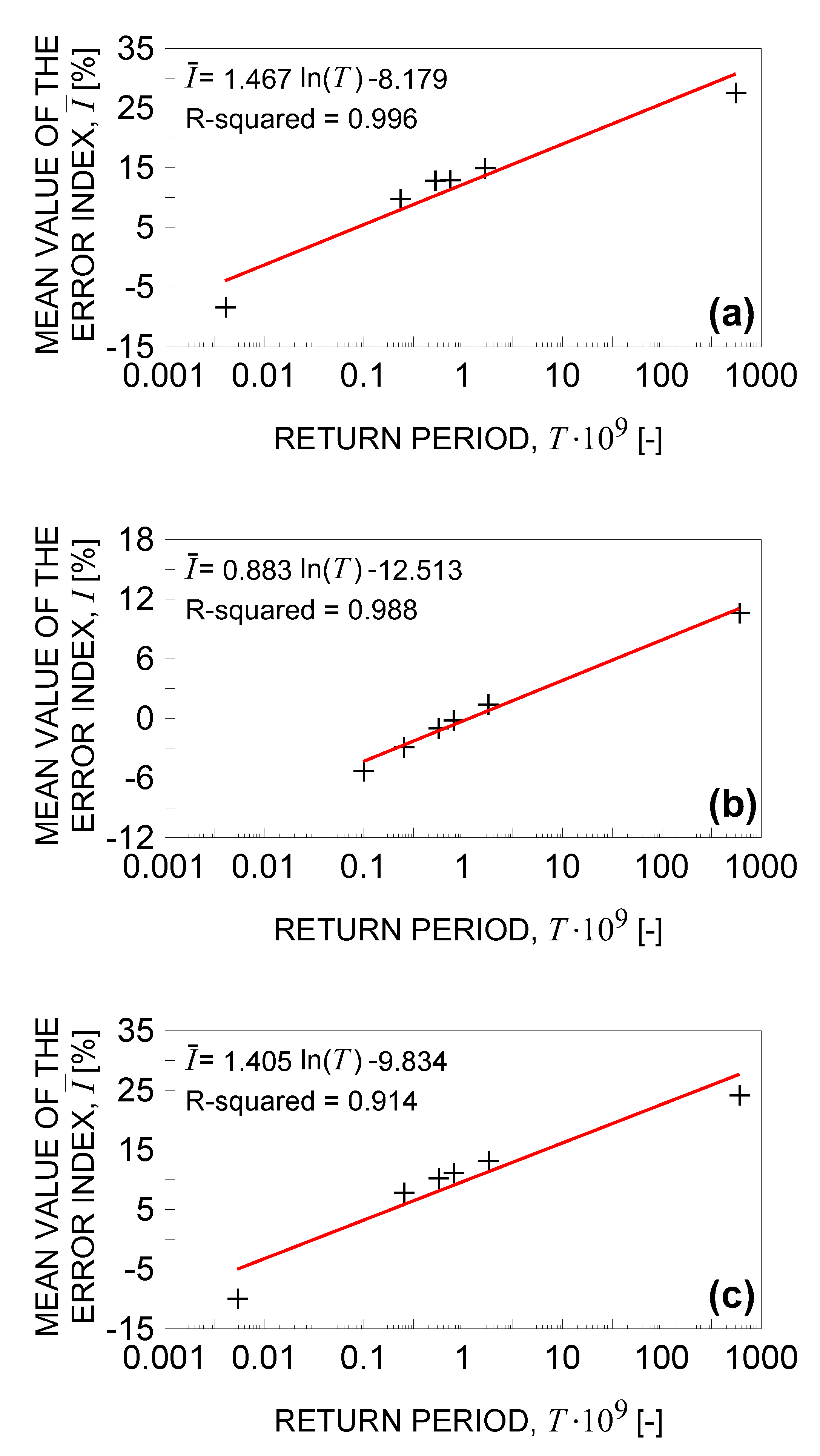
Figure 3.
Shear stress amplitude vs. equivalent normal stress amplitude acting on the critical plane for EN-GJS-400-18 DCI.
Figure 3.
Shear stress amplitude vs. equivalent normal stress amplitude acting on the critical plane for EN-GJS-400-18 DCI.
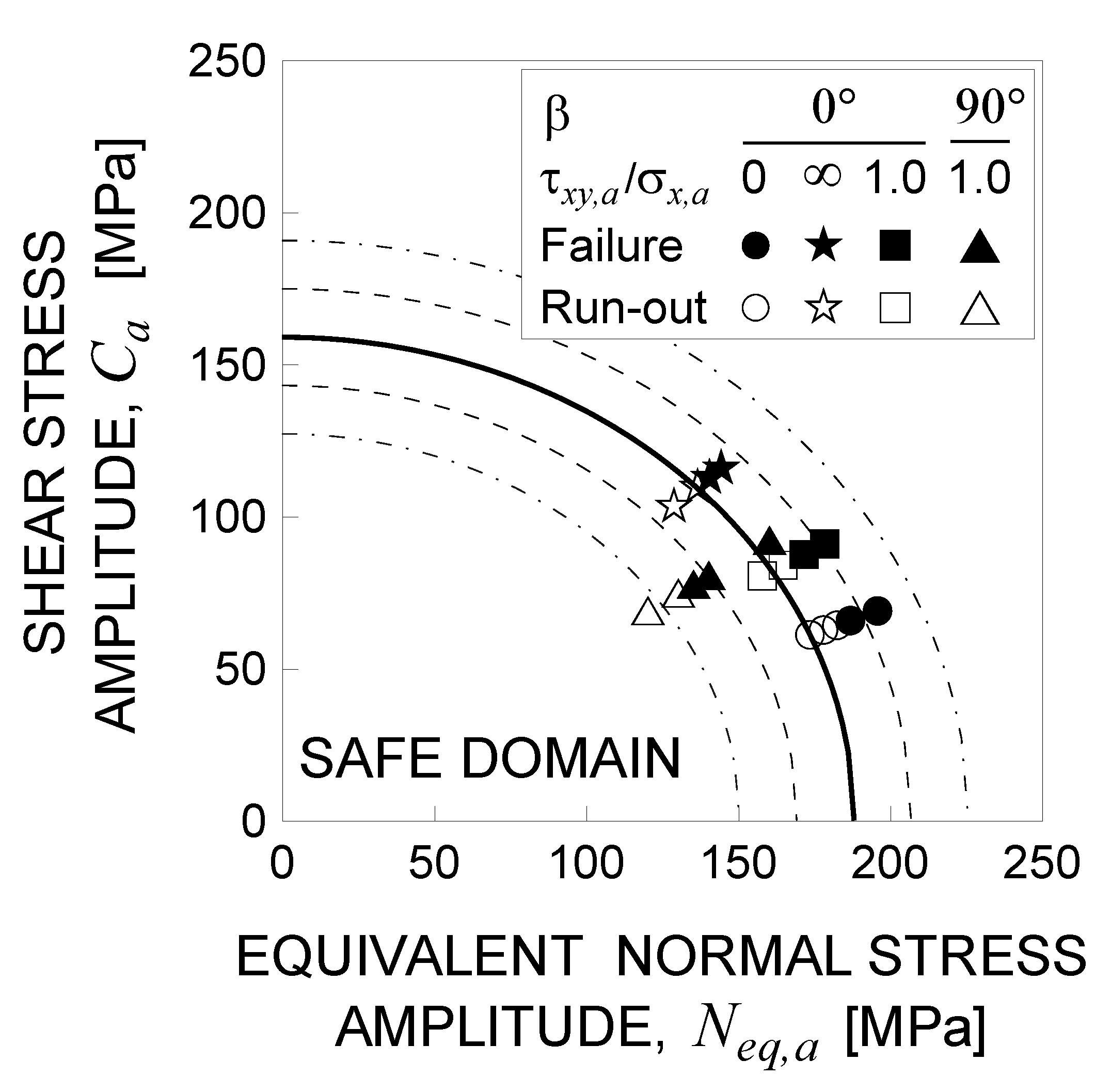
Figure 4.
Shear stress amplitude vs. equivalent normal stress amplitude acting on the critical plane for EN-GJS-600-3 DCI.
Figure 4.
Shear stress amplitude vs. equivalent normal stress amplitude acting on the critical plane for EN-GJS-600-3 DCI.

Figure 5.
Shear stress amplitude vs. equivalent normal stress amplitude acting on the critical plane for EN-GJS-700-2 DCI.
Figure 5.
Shear stress amplitude vs. equivalent normal stress amplitude acting on the critical plane for EN-GJS-700-2 DCI.
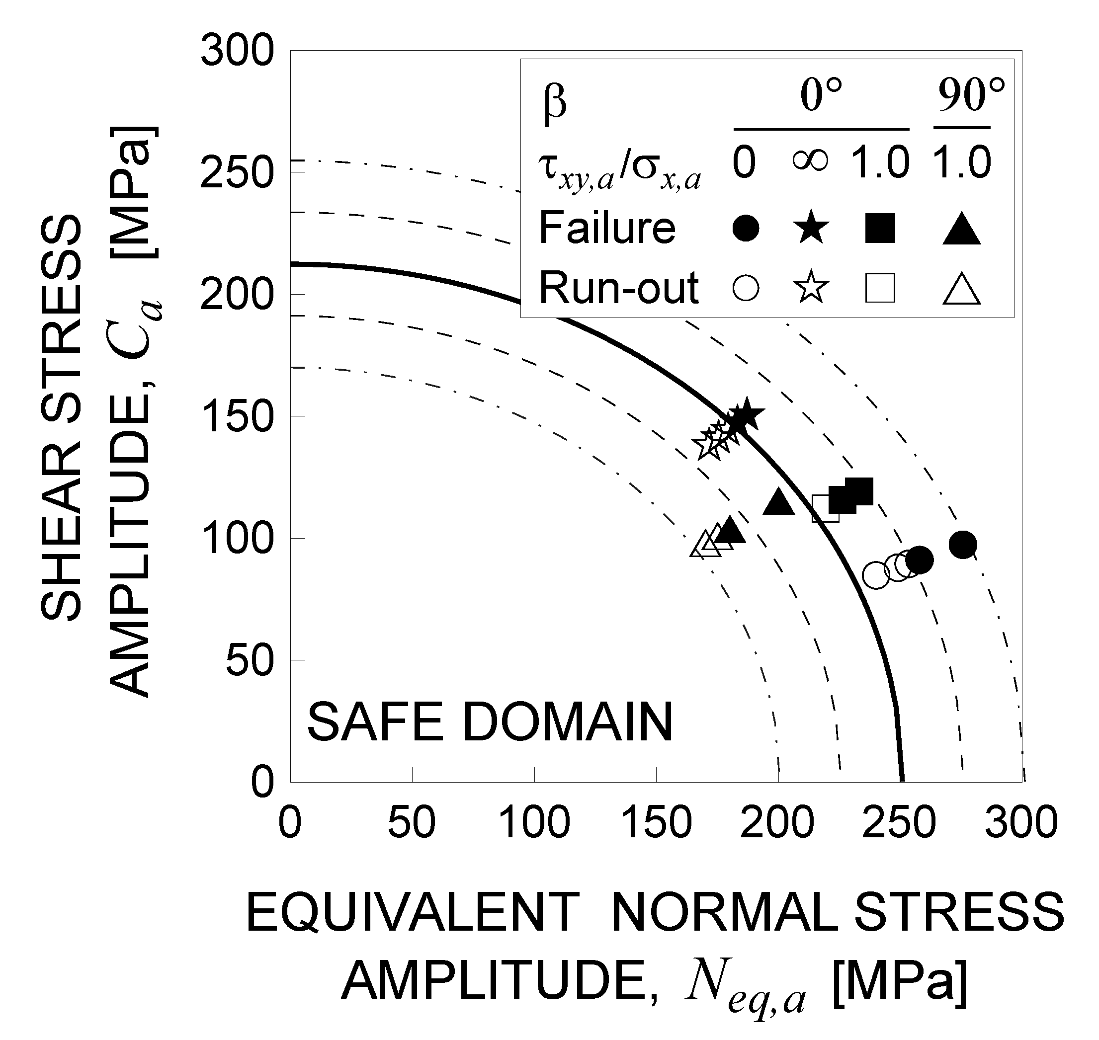
Figure 6.
Equivalent stress amplitude vs. test No. computed according to the present procedure for EN-GJS-400-18 DCI.
Figure 6.
Equivalent stress amplitude vs. test No. computed according to the present procedure for EN-GJS-400-18 DCI.
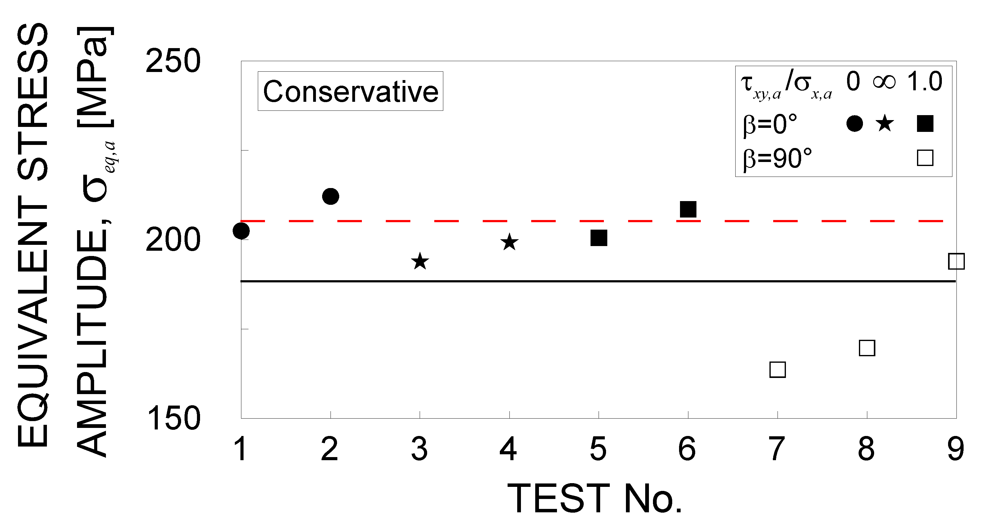
Figure 7.
Equivalent stress amplitude vs. test No. computed according to the present procedure for EN-GJS-600-3 DCI.
Figure 7.
Equivalent stress amplitude vs. test No. computed according to the present procedure for EN-GJS-600-3 DCI.
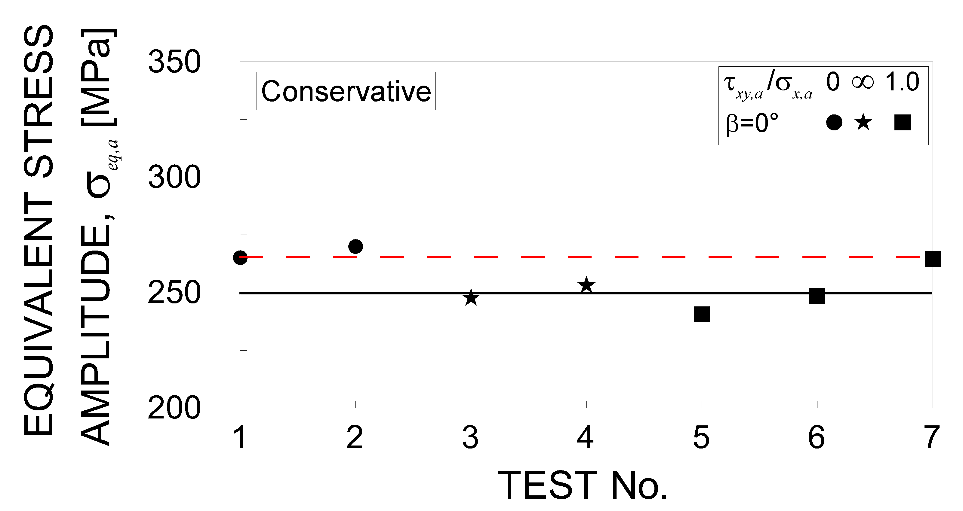
Figure 8.
Equivalent stress amplitude vs. test No. computed according to the present procedure for EN-GJS-700-2 DCI.
Figure 8.
Equivalent stress amplitude vs. test No. computed according to the present procedure for EN-GJS-700-2 DCI.


| MATERIAL | C | Si | Mn | P | S | Mg | Cu |
|---|---|---|---|---|---|---|---|
| EN-GJS-400-18 DCI | 3.72 | 2.14 | 0.32 | 0.01 | 0.02 | 0.04 | 0.04 |
| EN-GJS-600-3 DCI | 3.76 | 2.98 | 0.14 | 0.23 | 0.02 | 0.05 | 0.30 |
| EN-GJS-700-2 DCI | 3.77 | 2.99 | 0.44 | 0.02 | 0.11 | 0.06 | 0.47 |
| MATERIAL | [MPa] | Elongation [%] | [-] | [MPa] |
|---|---|---|---|---|
| EN-GJS-400-18 DCI | 418.0 | 25.0 | 186 | 205.0 |
| EN-GJS-600-3 DCI | 641.0 | 14.1 | 318 | 265.0 |
| EN-GJS-700-2 DCI | 734.0 | 8.0 | 318 | 280.0 |
Table 3.
Return period, prediction volume and fatigue limits for EN-GJS-400-18 DCI.
| [-] | [mm3] | [MPa] | [MPa] | |
|---|---|---|---|---|
| Symbol | Value | |||
| 5.54·104 | 1.41·103 | 171.14 | 144.44 | |
| 2.77·105 | 7.07·103 | 167.67 | 141.51 | |
| 5.54·105 | 1.41·104 | 166.31 | 140.36 | |
| 2.77·106 | 7.07·104 | 163.44 | 137.94 | |
| 3.09·1011 | 7.90·109 | 149.36 | 126.05 | |
| 1.67·10 | 4.27·10−1 | 205.00 | 173.01 | |
| 2.64·102 | 6.75 | 188.21 | 158.84 | |
Table 4.
Return period, prediction volume and fatigue limits for EN-GJS-600-3 DCI.
| [-] | [mm3] | [MPa] | [MPa] | |
|---|---|---|---|---|
| Symbol | Value | |||
| 6.50·104 | 1.41·103 | 258.32 | 218.02 | |
| 3.25·105 | 7.07·103 | 253.40 | 213.86 | |
| 6.50·105 | 1.41·104 | 251.47 | 212.23 | |
| 3.25·106 | 7.07·104 | 247.35 | 208.75 | |
| 3.63·1011 | 7.90·109 | 226.82 | 191.43 | |
| 1.01·104 | 2.29·102 | 265.00 | 223.65 | |
| 1.43·106 | 3.11·104 | 249.39 | 210.48 | |
Table 5.
Return period, prediction volume and fatigue limits for EN-GJS-700-2 DCI.
| [-] | [mm3] | [MPa] | [MPa] | |
|---|---|---|---|---|
| Symbol | Value | |||
| 6.54·104 | 1.41·103 | 233.86 | 197.37 | |
| 3.27·105 | 7.07·103 | 228.88 | 193.17 | |
| 6.54·105 | 1.41·104 | 226.96 | 191.54 | |
| 3.27·106 | 7.07·104 | 222.88 | 188.10 | |
| 3.65·1011 | 7.90·109 | 203.13 | 171.44 | |
| 2.94·10 | 6.35·10−1 | 280.00 | 236.31 | |
| 1.10·103 | 2.37·10 | 251.24 | 212.04 | |
Disclaimer/Publisher’s Note: The statements, opinions and data contained in all publications are solely those of the individual author(s) and contributor(s) and not of MDPI and/or the editor(s). MDPI and/or the editor(s) disclaim responsibility for any injury to people or property resulting from any ideas, methods, instructions or products referred to in the content. |
© 2022 by the author. Licensee MDPI, Basel, Switzerland. This article is an open access article distributed under the terms and conditions of the Creative Commons Attribution (CC BY) license (https://creativecommons.org/licenses/by/4.0/).
Share and Cite
MDPI and ACS Style
Ronchei, C. Fatigue Strength Estimation of Ductile Cast Irons Containing Solidification Defects. Metals 2023, 13, 83. https://doi.org/10.3390/met13010083
AMA Style
Ronchei C. Fatigue Strength Estimation of Ductile Cast Irons Containing Solidification Defects. Metals. 2023; 13(1):83. https://doi.org/10.3390/met13010083
Chicago/Turabian StyleRonchei, Camilla. 2023. "Fatigue Strength Estimation of Ductile Cast Irons Containing Solidification Defects" Metals 13, no. 1: 83. https://doi.org/10.3390/met13010083
Note that from the first issue of 2016, this journal uses article numbers instead of page numbers. See further details here.