In Situ Prediction of Metal Fatigue Life Using Frequency Change

Abstract

A reliable technique for rapid prediction of the remaining useful life (RUL) of components experiencing fatigue degradation is introduced. The approach is based on measuring the temperature signature of a component upon rapidly changing its operating frequency for a short period of time. The temperature variations caused by alterations in plastic work rate are correlated to the loading history. The efficacy of the approach is investigated by conducting a series of axial fatigue tests on stainless steel 316 specimens. The material characterization involves subjecting the material to a constant amplitude fatigue load at 4 Hz and 12 Hz frequencies. The operating frequency is temporarily adjusted to the characterization frequencies for a brief duration. During this period, the change in the slope of temperature rise is recorded. Subsequently, the operation frequency is reverted to its original state, and the remaining useful life is predicted based on the recorded data. The model provides predictions for operation frequencies of 6 Hz, 8 Hz, and 12 Hz, and notably, the error of predictions is consistently under 12% for all cases. The method allows the operator to reliably estimate the remaining usefulness for field applications without interrupting the operation.

1. Introduction

Fatigue degradation is inevitable in nearly all man-made machines that experience cyclic loading. Fatigue often results in unexpected failure disrupting operations and increasing maintenance costs with enormous implications for safety. To mitigate these risks, it is critical to accurately assess the remaining useful life (RUL) of components undergoing fatigue degradation. Given the critical role that RUL assessment plays in ensuring safety and reducing costs, industries are constantly searching for new and more efficient ways to predict the lifespans of their components. This paper aims to address the importance of RUL and introduces a thermodynamic-based framework that enables one to assess the RUL of working components without the need to remove a part or shut down the equipment.

The subject of estimation of metal fatigue life has been of interest for many years. Ahmadzadeh and Lundberg [1] wrote a comprehensive review of RUL methods and categorized the existing methods into four main groups: physics-based methods, empirical methods, data-driven approaches, and hybrid methods. Having examined the advantages and disadvantages of each method, the authors concluded that the selection of the method depends on the accuracy and availability of data. The data-driven method is suggested for cases where an abundance of data is accessible, but high accuracy is not a major concern; however, for cases where large amounts of data on damage estimation are not on hand, physics-based models are a more reliable answer.

Bagul [2] categorizes physics-based methodologies into fundamental classifications comprising physical models, statistical models, Kalman and particle filtering, and nonlinear dynamics. Noteworthy contributions within the domain of physical models include the work of Li et al. [3], which focuses on damage assessment for rolling element bearings. Their approach leverages vibration feedback and Paris’s formula to construct a robust physics-based model. Furthermore, Oppenheimer and Loparo [4] have developed a life model grounded in the Forman crack growth law, serving as a valuable tool for assessing damage in cracked rotor shafts. Within the statistical models’ category, there exists a taxonomy encompassing proportion hazards models [5], logistic regression models [6], and cumulative damage models [7]. Kuncham et al. [8] developed an online model that utilizes an extended Kalman filter along with Paris’s equation to assess the condition of a structure undergoing cyclic loading. A Kalman filter allows the system status to be evaluated at each state based on previous data acquired. It is crucial to emphasize that the efficacy of most physics-based models hinges upon meticulous system parameter characterization, which entails an in-depth understanding of the governing physical equations and the consideration of ancillary factors like corrosion [1].

Additionally, Bagul [2] delves into data-driven methodologies, dividing them into various categories, including multivariate statistical techniques, black box methodologies, graphical models, and signal analysis. However, it is imperative to underscore that data-driven methods heavily rely on the availability of extensive raw data.

Hybrid methodologies are currently witnessing an upward trend because of their capacity to harness the synergistic potential of two or more prediction techniques. Recent research endeavors have prominently featured the integration of diverse approaches within hybrid frameworks. These approaches encompass the amalgamation of Fourier transform with neural networks [9], the fusion of fuzzy logic with neural networks [10], and the amalgamation of statistical models with neural networks [11], among others [1]. Hybrid methods may have one or more limitations of the other mentioned methods; however, they may increase the processing time and accuracy of the predictions. Presented below are additional exemplifications of the aforementioned methodological paradigms.

Li and Lee [12] devised a model to estimate crack size as a function of load and stress concentration. They used a crack growth model based on Paris’s law to investigate the RUL of gears with existing cracks. Todinov [13] proposed a new equation that considers the density of flaws in a randomly shaped component and introduced the maximum level allowable in the component to achieve the minimum failure probability. Medjaher et al. [14] proposed a data-driven RUL method for analyzing the degradation of bearings operating at stable conditions. The method includes two phases: assessing the degradation behavior by gathering data and implementing the outcome of the first phase for estimation purposes. The authors utilize Gaussian mixture and hidden Markov models that allow one to use the hidden states to describe the degradation evolution.

On another front, physics-based studies on fatigue behavior that apply the laws of thermodynamics have received considerable attention in recent years. Naderi et al. [15] introduced generated entropy during fatigue processes as an index to evaluate the life of components. They demonstrated it is a material property and called it fracture fatigue entropy (FFE). Numerous works have been reported by researchers such as Wang et al. [16], Huang et al. [17], and others aiming to find the threshold at which fracture is likely to occur. The validity of this thermodynamic-based framework for various materials and conditions has been revealed [18,19,20]. Recently, Amooie et al. [21] showed that accumulated entropy up to fracture remains fairly constant in a variable frequency fatigue loading.

While a substantial body of research has been devoted to studying the base principles of thermodynamics in fatigue, a practical means for evaluating the RUL of mechanical components remains elusive. This paper is devoted to fulfilling this need and aims to introduce an innovative approach for evaluating the remaining useful life (RUL) of components subjected to fatigue loading without interrupting or halting the operation. The approach leverages the principles of fatigue thermodynamics and damage entropy to formulate a novel method for estimating the damage state of the component or material while it is in operation. In the next section, the theory and formulation of this new method are introduced. Section 3 will give a brief explanation of the experimental procedure. Section 4 is devoted to experimental results and comparison with the theory, and Section 5 presents the main findings of this study.

2. Theory and Formulation

2.1. Thermodynamics of Fatigue

Irreversible fatigue degradation can be investigated in the framework of thermodynamics. The accumulated entropy generation during fatigue is an index of the irreversibility of a system and can be computed using the following equation [22,23]:

$${\gamma }_f={{\displaystyle \int }}_0^{t_f}\frac{{\dot{Q}}_{gen}}{T}dt$$

(1)

where ${\gamma }_f$ is the accumulated non-negative entropy generation up to fracture. ${\dot{Q}}_{gen}$ is the generated energy inside the material, and T represents the temperature in Kelvin scale; $t$ denotes time, and $t_f$ is the time at fracture.

It has been shown that the accumulated entropy up to fatigue fracture, the so-called fracture fatigue entropy (FFE), is nearly constant, and the entropy accumulates linearly up to fracture [15]. Thus, an entropic damage parameter can be defined as:

$${\omega }_N=\frac{{\gamma }_N}{\mathrm{FFE}}=\frac{N}{N_f}=N^{\ast }$$

(2)

where ${\omega }_N$ is entropic damage parameter, and ${\gamma }_N$ represent the accumulated entropy up to cycle $N$. $N_f$ is the number of cycles to failure, and $N^{\ast }$ is the normalized life associated with cycle $N$th.

To evaluate the cyclic entropy accumulation, the heat generation (${\dot{Q}}_{gen}$) should be calculated. Among different methods, the $R_{\theta }$ approach has been widely used to estimate ${\dot{Q}}_{gen}$ using the rate of temperature rise at the beginning of the fatigue process [24]:

$${\dot{Q}}_{gen}=\rho c_p{R}_{\theta }$$

(3)

where $\rho$ is density, and $c_p$ is the specific heat capacity. Equation (3) shows that $R_{\theta }$ can be used to estimate heat generation during the fatigue process. It has been shown that a repeating run–stop–cooldown (RSC) can be used to characterize a given material’s fatigue behavior [25]. RCS involves repeated stops of a fatigue load allowing the specimen to cool down to the ambient temperature and then resuming again. The $R_{\theta }$ increases linearly with the number of cycles, N, until failure occurs [25]. This linear trend of $R_{\theta }$ is utilized to estimate the remaining useful life. The procedure is described in the next section.

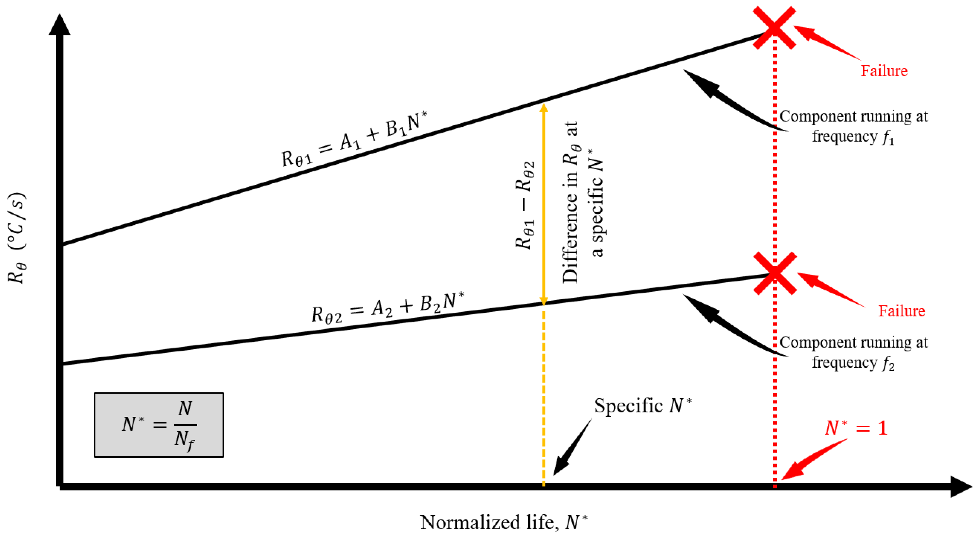
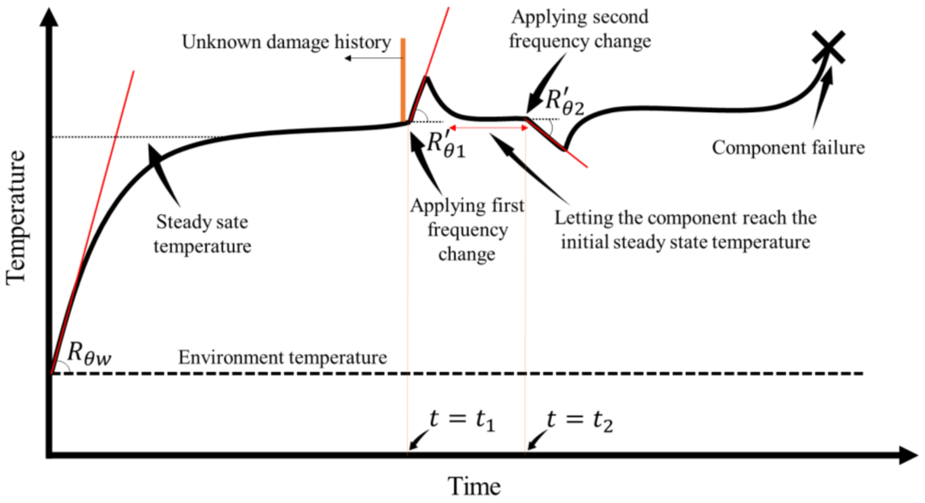
2.2. Influence of Rapid Change in Frequency

In a repeated RSC procedure, the $R_{\theta }$ increases linearly with respect to the number of cycles as:

$$R_{\theta }=A+BN$$

(4)

where $A$ is the initial value for a pristine specimen, and $B$ is a constant. Figure 1 illustrates the trend of $R_{\theta }$ at two different frequencies, $f_1$ and $f_2$, $f_1>f_2$. $R_{\theta }$ changes with respect to normalized life, $N^{\ast }$, and can be determined as:

$$\{\begin{array}{c}{R}_{{\theta }_1}=A_1+B_1{N}^{\ast }\\ R_{{\theta }_2}=A_2+B_2{N}^{\ast }\end{array}$$

(5)

Referring to Figure 2, consider a component operating at its normal operating frequency $f_w$. Its temperature rises initially at a rate of $R_{{\theta }_w}$ and reaches the stabilization condition at the steady-state temperature $T_{ss}$. While operating in steady state and in balance, we have:

$${\dot{Q}}_{out}={\dot{Q}}_{gen}=\rho c_p{R}_{{\theta }_w}$$

(6)

Now, if the frequency changes suddenly during steady state at $t=t_i$, the temperature starts to change at the rate of $R_{\theta }^{\prime }$. Upon changing the frequency at $t=t_i^{+}$, the conservation energy would require:

$$\rho c_p{R}_{\theta }^{\prime }={\dot{Q}}_{gen}-{\dot{Q}}_{out}$$

(7)

where ${\dot{Q}}_{out}$ is the heat dissipated to the surroundings. At $t=t_i^{+}$, ${\dot{Q}}_{out}$ remains fairly constant because of no instant change in temperature, and it can be replaced using Equation (6):

$${\dot{Q}}_{gen}=\rho c_p\left(R_{{\theta }_w}+R_{\theta }^{\prime }\right)$$

(8)

Note that $R_{{\theta }_w}$ is unknown, and it is necessary to employ a technique to eliminate it from the equations in order to determine the remaining useful life. Now, assume that after attaining a steady state, the operator manually increases the frequency to $f_1>f_w$ at $t=t_1$ for only a few seconds. As a result, the temperature rises at the rate of $R_{{\theta }_1}^{\prime }$. Next, the operator reduces the frequency to its original working frequency $f_w$ and the specimen cooldowns to the steady-state temperature. Next, the frequency is decreased to $f_2<f_w$ at $t=t_2$. The temperature drops at the rate of $R_{{\theta }_2}^{\prime }$, and again, after a few seconds, the temperature returned to $f_w$, so that the temperature rises back up to $T_{ss}$. It is assumed that the expended life in this procedure, from $t_1$ to $t_2$, is negligible in comparison to the total life, $N_f$. Therefore, according to Equation (2), the state of damage, ${\omega }_N$, and consequently $N^{\ast }$ at $t=t_1$ and $t=t_2$ remain nearly unchanged.

Using Equation (8), the heat generation at $t=t_1$ and $t=t_2$ are:

$$\{\begin{array}{c}{\dot{Q}}_{gen,1}=\rho c_p\left(R_{{\theta }_w}+R_{{\theta }_1}^{\prime }\right)\\ {\dot{Q}}_{gen,2}=\rho c_p\left(R_{{\theta }_w}-R_{{\theta }_2}^{\prime }\right)\end{array}$$

(9)

If the machine was working at the frequency of $f_1$ or $f_2$ instead of $f_w$ from the beginning of the fatigue process, its temperature would have increased at the rate of $R_{\theta }{}_1$ or $R_{\theta }{}_2$, respectively. The heat generation in those cases could be estimated as:

$$\{\begin{array}{c}{\dot{Q}}_{gen,1}=\rho c_p{R}_{\theta }{}_1\\ {\dot{Q}}_{gen,2}=\rho c_p{R}_{\theta }{}_2\end{array}$$

(10)

Considering that, at each frequency, the rate of heat generation is unique for a specific $N^{\ast }$, the heat generation is the same in these two scenarios; therefore, substituting Equation (10) into Equation (9) yields:

$$\{\begin{array}{c}{R}_{{\theta }_1}=R_{{\theta }_w}+R_{{\theta }_1}^{\prime } \left(a\right)\\ R_{{\theta }_2}=R_{{\theta }_w}-R_{{\theta }_2}^{\prime } \left(b\right)\end{array}$$

(11)

Subtracting Equation (11b) from Equation (11a) yields:

$$R_{{\theta }_1}-R_{{\theta }_2}=R_{{\theta }_1}^{\prime }+R_{{\theta }_2}^{\prime }$$

(12)

The right-hand side of Equation (12), ($R_{{\theta }_1}^{\prime }+R_{{\theta }_2}^{\prime })$ is known and can be obtained from a frequency change test. Referring to Figure 1 and using Equations (5) and (12), the corresponding expended normalized life can be calculated and estimated as:

$$N^{\ast }=\frac{\left(R_{{\theta }_1}^{\prime }+R_{{\theta }_2}^{\prime }\right)-\left(A_1-A_2\right)}{\left(B_1-B_2\right)}$$

(13)

Equation (13) reveals that the expended life can be obtained by measuring the rate of temperature change with frequency change and using the material’s characterization at two different frequencies. This method can be applied to find the remaining useful life without knowing the history of loading since $R_{{\theta }_w}$ is eliminated. This is because damage is a state variable and independent of the loading path. The method proposed in this study hinges on estimating the generated entropy within the material by analyzing its thermal responses. In this study, the application of the method for constant amplitude fatigue load is investigated. However, the efficacy of the methods for variable amplitude loading and load cases with unknown loading history needs further investigation.

3. Experimental Verification

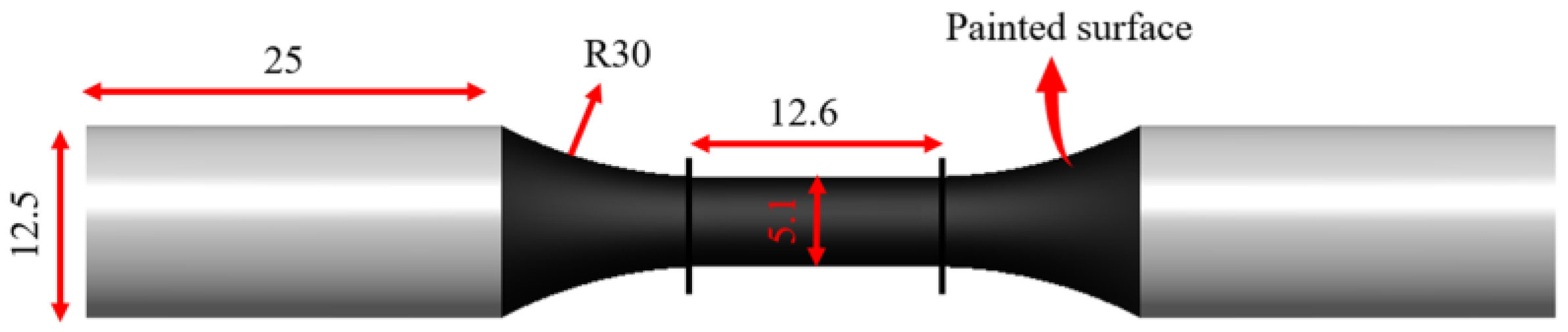
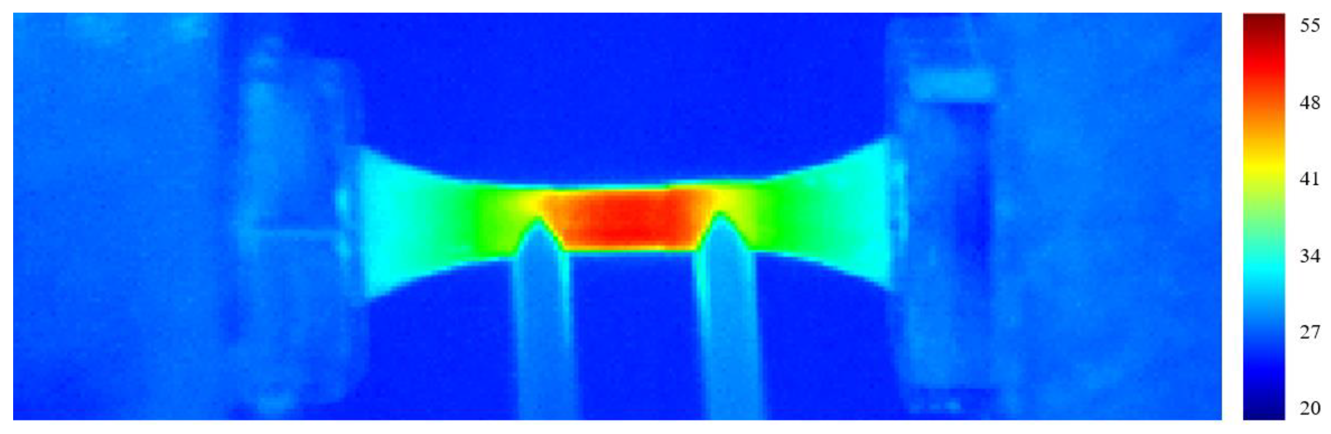
3.1. Material and Test Equipment

The specimens used for experimental validation are made of stainless steel (SS) 316. This method’s applicability extends beyond the current material to encompass a wide array of materials. The foundational theory and characterization process retain their consistency, ensuring adaptability to diverse material types. It is rooted in understanding damage evolution and alterations in material microstructure caused by fatigue and the capacity of a material to generate entropy. However, a critical prerequisite is that the material must undergo enough temperature rise during fatigue to facilitate the application of this method. Many metals and composite materials inherently generate ample heat during fatigue, providing the necessary temperature rise essential for analysis. The SS 316 materials are machined in the shape of cylindrical dog bones. The material’s chemical composition is presented in

Table 1. Chemical composition of SS 316 provided by the supplier *.

Material	Fe	C	Cr	Mo	Ni	Mn	P	S	Si
SS 316	82 Max	0.08	18 Max	3 Max	14 Max	2	0.045	0.03	1

* www.OnlineMetals.com accessed on 1 March 2023.

. Static tests are carried out to measure the mechanical properties of the specimens. The material has an ultimate strength of 640 MPa, yield strength of 520 MPa, and Young’s modulus of 171 GPa. The mechanical and physical properties of the specimens are summarized in

Table 2. Mechanical and physical properties of SS 316.

Material	Density $\mathit{\rho }$ (Kg/m3)	Thermal Conductivity K (W/m·K)	Specific Heat Capacity C (J/kg·K)	Young’s Modulus E (GPa)	Ultimate Strength ${\mathit{\sigma }}_{\mathit{u}}$ (MPa)	Yield Strength ${\mathit{\sigma }}_{\mathit{y}}$ (MPa)
SS 316	8000 *	15.3 *	490 *	171	640	520

* Provided by supplier available on www.OnlineMetals.com.

.

Specimens are prepared using ASTM E466-15 [26] for constant amplitude axial fatigue tests. The dimensions of the tested dog bones are presented in Figure 3. Specimens are polished up to 0.2 µm, and a thin layer of black paint is sprayed on the gauge section of the specimen to increase the emissivity.

The TestResources hydraulic fatigue tester with a 25 kN load capacity is used to conduct static and fatigue tests. Figure 4 shows a test setup of a specimen undergoing loading. An infrared (IR) camera (FLIR A600 series) with a resolution of 640 × 480 pixels, thermal sensitivity of <0.05 °C at 30 °C, accuracy of ±2 °C or ±2% of reading, and data acquisition rate of up to 200 Hz is employed to record and monitor temperature fluctuations on the specimen’s surface, which allows for detailed and precise temperature measurements.

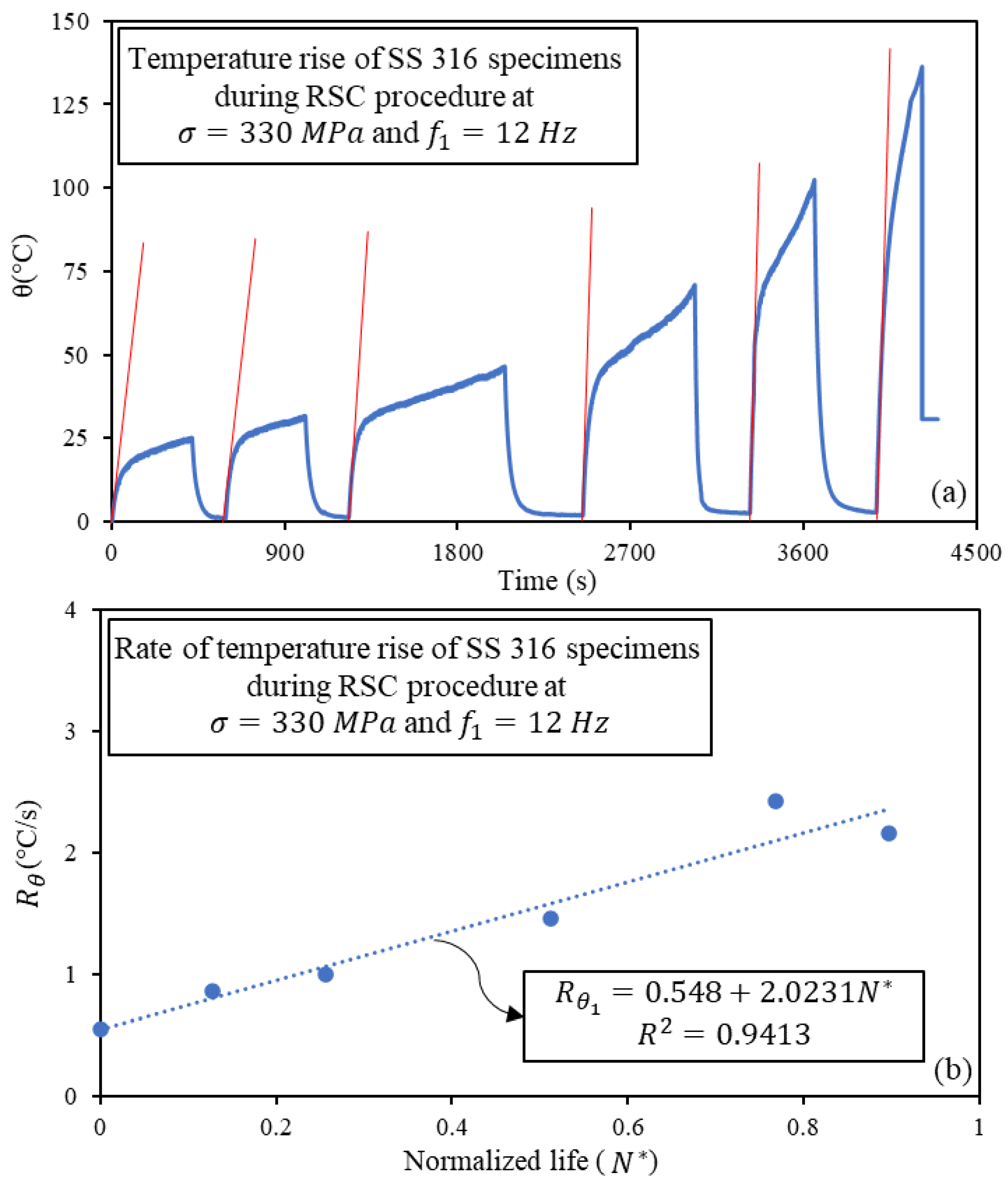
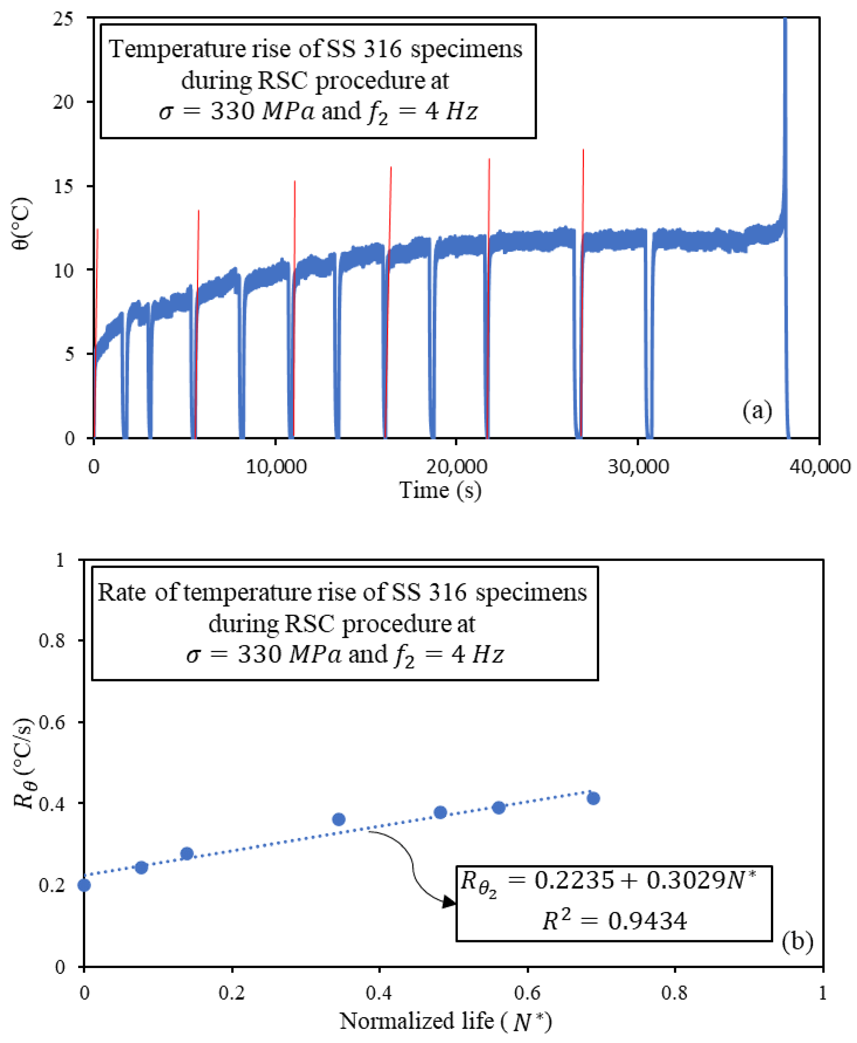
3.2. Characterization at Different Frequencies

As described in the previous section, the component should be characterized at a constant stress level and at two different frequencies using the RSC procedure to evaluate the remaining useful life. In this method, the test is stopped at different stages of fatigue, the specimen is allowed to cool down to the ambient temperature, and then, the test is resumed. The rate of temperature rise at the beginning of each stage is measured. Using Equation (5), the relation between the normalized life ($N^{\ast }$) and rate of temperature rise ($R_{\theta }$) is characterized at two different frequencies. The tests are conducted at a constant amplitude of 330 MPa at frequencies of 12 Hz and 4 Hz. The fatigue loads are sinusoidal with the load ratio of L_R = −1.

Figure 5a shows the rise and drop of temperature during the RSC procedure at the frequency of 12 Hz. The increasing trend of $R_{\theta }$ is shown in Figure 5b, where the relation between $R_{{\theta }_1}$ and normalized life ($N^{\ast }$) is determined. It clearly indicates that the rate of temperature rise increases because of growth in damage and microstructural change in material. The characterization process remains unaffected by the intervals chosen for the run–stop–cooldown (RSC) procedure. Damage and microstructure changes are contingent upon the number of fatigue cycles, resulting in a consistent trend in the $R_{\theta }$, regardless of the chosen intervals. Various intervals are chosen for the RSC procedure to demonstrate this inherent independence.

Figure 6a represents the temperature growth during the RSC procedure at the frequency of 4 Hz. It shows that after each interval, the temperature reaches a higher value. However, the temperature increase before reaching the final stage of fatigue at 4 Hz, 12 °C, is significantly lower than the maximum temperature observed during the RSC procedure at the 12 Hz frequency, which reaches 65 °C. Figure 6b shows how the rate of temperature rise at each interval increases throughout the fatigue process, as presented in the form of a relation between $R_{{\theta }_2}$ and the normalized life. The constants in Equation (5) for $R_{{\theta }_1}$ and $R_{{\theta }_2}$ are summarized in

Table 3. Characterization of the model at different frequencies.

Frequency (Hz)	$\mathit{A}$	$\mathit{B}$
12	0.5480	2.0231
4	0.2235	0.3029

.

3.3. RUL Assessment Procedure

The first step for developing an RUL assessment procedure is to characterize the material’s thermographic behavior using two reference frequencies, as outlined in the preceding section. A pristine specimen is subjected to cyclic loading at the characterized stress level of 330 MPa. The testing process employs working frequencies of 6 Hz, 8 Hz, and 10 Hz, which are selected to fall between the characterization frequencies.

Once the specimen reaches a steady-state temperature, frequency variations are introduced. The frequency change involves increasing the frequency to 12 Hz for a brief duration and, then, returning it to the working frequency to allow the material to reach the previous steady-state temperature. Subsequently, the frequency is decreased to the second reference frequency of 4 Hz. After a few seconds, the test frequency is reset to its initial working frequency. This procedure is repeated multiple times at different intervals throughout the fatigue process. By using Equation (13) and the obtained slopes of temperature rise/drop caused by frequency change in this procedure, the expended life and remaining useful life can be estimated. The next section is devoted to discussing the results.

4. Results and Discussion

Figure 7 shows a typical temperature profile of a specimen under fatigue loading. The maximum temperature occurs at the gauge section. The values of $R_{{\theta }_1}^{\prime }$ and $R_{{\theta }_2}^{\prime }$ are measured when the working frequency is changed for a few seconds, and these values are used to find the RUL based on Equation (13). Three different working frequencies—6 Hz, 8 Hz, and 10 Hz—are used to examine the method, and the results are presented as follows.

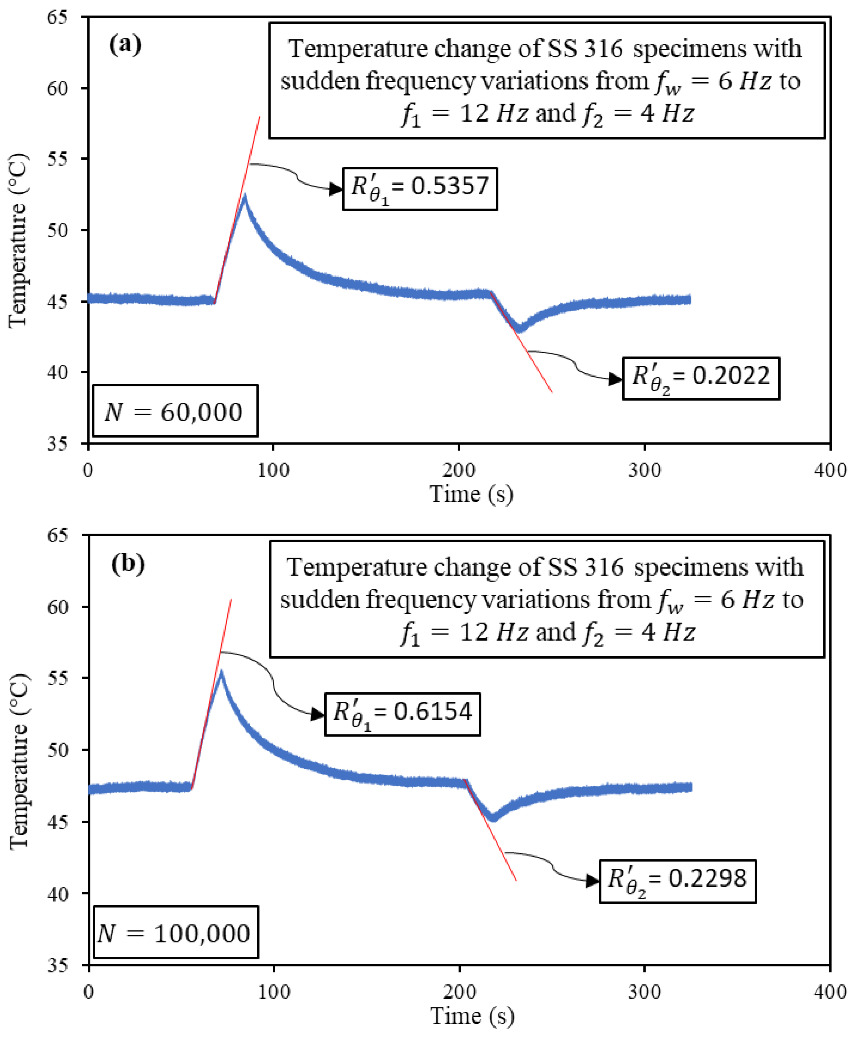
4.1. Working Frequency 6 Hz

The RUL assessment procedure is applied at different intervals of a single fatigue test at the working frequency of 6 Hz. Figure 8 illustrates the temperature profile during the RUL estimation process at two different intervals, after (a) $N$ = 60,000 cycles and (b) $N$ = 100,000 cycles. The graph demonstrates the sequence of frequency changes and their corresponding impact on temperature variations. Initially, the frequency is adjusted to 12 Hz for a brief duration, after which it is reverted back to 6 Hz, allowing the material to attain its original steady-state temperature. Subsequently, the frequency is reduced to 4 Hz for a short period before returning to the initial value of 6 Hz. The procedure was repeated at various intervals throughout the fatigue process to evaluate the method’s efficacy. In the end, the experiment was continued until the specimen eventually fractured, allowing for the determination of its fatigue life.

Table 4. Prediction of expended life using Equation (13) at the frequency of 6 Hz.

N	${\mathit{R}}_{{\mathit{\theta }}_1}^{\prime }$	${\mathit{R}}_{{\mathit{\theta }}_2}^{\prime }$	$\mathbf{Estimated} {\mathit{N}}^{\ast }$	$\mathbf{Actual} {\mathit{N}}^{\ast }$	Error (% of Actual Life)
10,000	0.3559	0.1186	0.087	0.023	6.4
30,000	0.4706	0.1470	0.170	0.066	10.4
60,000	0.5357	0.2022	0.240	0.132	10.8
100,000	0.6154	0.2298	0.303	0.218	8.5
177,000	0.6513	0.2559	0.339	0.385	−4.6
210,000	0.6691	0.2576	0.350	0.458	−10.8
350,000	0.9206	0.5089	0.642	0.761	−11.9

serves to consolidate the data obtained from the RUL assessment procedure at different fatigue intervals. It presents the specific life at which frequency changes are applied during the testing, along with corresponding observations for $R_{{\theta }_1}^{\prime }$ and $R_{{\theta }_2}^{\prime }$ and the results for $N^{\ast }$ at each stage of fatigue degradation. The error between the estimated $N^{\ast }$ and the actual $N^{\ast }$ is reported. As can be seen, the maximum error recorded is 11.9% of actual life.

4.2. Working Frequency 8 Hz

The testing process described earlier is also conducted for a working frequency of 8 Hz. The results are graphically presented in Figure 9 at two different life stages, showing the temperature profile during the RUL estimation process at 8 Hz. The figure demonstrates the frequency changes implemented and their corresponding effects on the temperature variations. Similar to the previous case, the frequency is first adjusted to 12 Hz for a short duration, followed by a return to the working frequency of 8 Hz to allow the material to reach its initial steady-state temperature. Subsequently, the frequency is reduced to 4 Hz briefly before reverting to the original working frequency of 8 Hz. A summary of the RUL estimation process at the working frequency of 8 Hz is presented in

Table 5. Prediction of expended life using Equation (13) at the frequency of 8 Hz.

N	${\mathit{R}}_{{\mathit{\theta }}_1}^{\prime }$	${\mathit{R}}_{{\mathit{\theta }}_2}^{\prime }$	$\mathbf{Estimated} {\mathit{N}}^{\ast }$	$\mathbf{Actual} {\mathit{N}}^{\ast }$	Error (% of Actual Life)
10,000	0.2560	0.2626	0.113	0.036	7.7
30,000	0.3467	0.3208	0.199	0.105	9.4
72,000	0.3819	0.4883	0.317	0.250	6.7
106,000	0.5122	0.5334	0.419	0.367	5.2
140,000	0.6581	0.6990	0.600	0.484	11.6
183,000	0.6986	0.7027	0.626	0.633	−0.7

. The maximum error observed for this case is 11.6% of actual life.

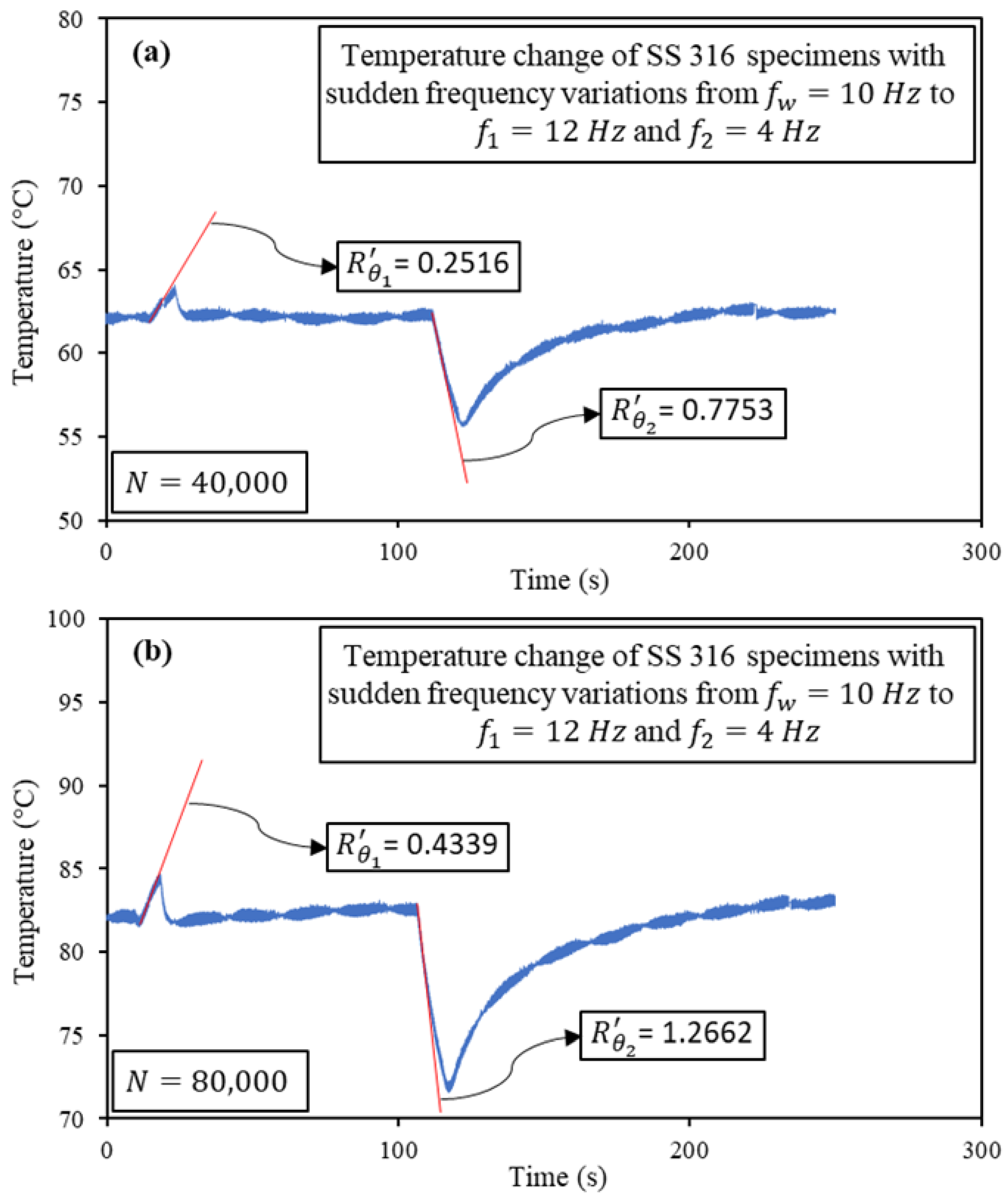
4.3. Working Frequency 10 Hz

The third test condition is for a working frequency of 10 Hz. Tests were conducted at reference frequencies of 12 Hz and 4 Hz. Two frequency manipulation diagrams are presented in Figure 10, and a summary of the estimated and experimental $N^{\ast }$ is presented in

Table 6. Prediction of expended life using Equation (13) at the frequency of 10 Hz.

N	${\mathit{R}}_{{\mathit{\theta }}_1}^{\prime }$	${\mathit{R}}_{{\mathit{\theta }}_2}^{\prime }$	$\mathbf{Estimated} {\mathit{N}}^{\ast }$	$\mathbf{Actual} {\mathit{N}}^{\ast }$	Error (% of Actual Life)
10,000	0.0975	0.2660	0.023	0.096	−7.3
33,000	0.2501	0.6905	0.358	0.302	5.6
40,000	0.2516	0.7753	0.408	0.366	4.2
45,000	0.2929	0.7958	0.446	0.412	3.4
55,000	0.3199	0.9194	0.532	0.503	2.9
65,000	0.3255	1.0113	0.589	0.595	−0.6
80,000	0.4339	1.2662	0.800	0.732	6.8

. The maximum reported error is 7.3% of the actual life.

5. Conclusions

The present paper introduces an innovative approach for the rapid evaluation of components’ remaining useful life (RUL), leveraging the materials’ thermographic behavior during fatigue degradation. This method entails initial characterization testing to establish the material’s behavior. Once characterized, the RUL can be promptly estimated. In this study, we specifically investigated the fatigue behavior of SS 316. The model’s applicability can be tested with any material; however, it is essential to ensure that the test generates a sufficient temperature rise for the application of the proposed method. The experimental process requires characterizing the material at two different frequencies. The model takes advantage of the linear damage accumulation with respect to the normalized life of the component. Characterization processes are conducted at frequencies of 12 and 4 Hz, and the experimental verification is conducted for working frequencies of 6, 8, and 10 Hz. The results show that the method can reliably assess the remaining useful life, and the error between the estimated life and real life is less than 12% of the total life of the samples. The fatigue tests are performed under constant amplitude loads. To extend the model’s applicability to variable amplitude loading and fatigue loading scenarios with unknown loading histories, further investigation and validation are required.

The notable advantage of this method lies in its ability to predict the remaining useful fatigue without interrupting the operation of the machine. The RUL can be reliably estimated by temporarily fluctuating the working frequency and employing thermographic sensors. This nonintrusive methodology affords real-time evaluations of component health, enabling timely maintenance interventions and proactive decision-making.

References

1. Ahmadzadeh, F.; Lundberg, J. Remaining useful life estimation. Int. J. Syst. Assur. Eng. Manag. 2014, 5, 461–474. [Google Scholar] [CrossRef]
2. Bagul, Y.G. Assessment of Current Health and Remaining Useful Life of Hard Disk Drives; Northeastern University: Boston, MA, USA, 2009. [Google Scholar]
3. Li, Y.; Billington, S.; Zhang, C.; Kurfess, T.; Danyluk, S.; Liang, S. Adaptive prognostics for rolling element bearing condition. Mech. Syst. Signal Process. 1999, 13, 103–113. [Google Scholar] [CrossRef]
4. Oppenheimer, C.H.; Loparo, K.A. Physically based diagnosis and prognosis of cracked rotor shafts. In Proceedings of the Component and Systems Diagnostics, Prognostics, and Health Management II, Orlando, FL, USA, 16 July 2002; Volume 4733, pp. 122–132. [Google Scholar]
5. Wang, W. A model to predict the residual life of rolling element bearings given monitored condition information to date. IMA J. Manag. Math. 2002, 13, 3–16. [Google Scholar] [CrossRef]
6. Liao, H.; Zhao, W.; Guo, H. Predicting remaining useful life of an individual unit using proportional hazards model and logistic regression model. In Proceedings of the RAMS'06. Annual Reliability and Maintainability Symposium, Newport Beach, CA, USA, 23–26 January 2006; pp. 127–132. [Google Scholar]
7. Usynin, A.V. A generic prognostic framework for remaining useful life prediction of complex engineering systems. Doctoral dissertation, The University of Tennessee, Knoxville, TN, USA, 2007. [Google Scholar]
8. Kuncham, E.; Sen, S.; Kumar, P.; Pathak, H. An online model-based fatigue life prediction approach using extended Kalman filter. Theor. Appl. Fract. Mech. 2022, 117, 103143. [Google Scholar] [CrossRef]
9. Lao, H.; Zein-Sabatto, S. Analysis of vibration signal’s time-frequency patterns for prediction of bearing’s remaining useful life. In Proceedings of the 33rd Southeastern Symposium on System Theory (Cat. No. 01EX460), Athens, OH, USA, 18–20 March 2001; pp. 25–29. [Google Scholar]
10. El-Koujok, M.; Gouriveau, R.; Zerhouni, N. From monitoring data to remaining useful life: An evolving approach including uncertainty. In Proceedings of the 34th European Safety Reliability & Data Association, ESReDA Seminar and 2nd Joint ESReDA/ESRA Seminar on Supporting Technologies for Advanced Maintenance Informaiton Management, San Sebastian, Spain, May 2008; pp. 1–12. [Google Scholar]
11. Tian, Z. An artificial neural network method for remaining useful life prediction of equipment subject to condition monitoring. J. Intell. Manuf. 2012, 23, 227–237. [Google Scholar] [CrossRef]
12. Li, C.J.; Lee, H. Gear fatigue crack prognosis using embedded model, gear dynamic model and fracture mechanics. Mech. Syst. Signal Process. 2005, 19, 836–846. [Google Scholar] [CrossRef]
13. Todinov, M. Limiting the probability of failure for components containing flaws. Comput. Mater. Sci. 2005, 32, 156–166. [Google Scholar] [CrossRef]
14. Medjaher, K.; Tobon-Mejia, D.A.; Zerhouni, N. Remaining useful life estimation of critical components with application to bearings. IEEE Trans. Reliab. 2012, 61, 292–302. [Google Scholar] [CrossRef]
15. Naderi, M.; Amiri, M.; Khonsari, M. On the thermodynamic entropy of fatigue fracture. Proc. R. Soc. A Math. Phys. Eng. Sci. 2010, 466, 423–438. [Google Scholar] [CrossRef]
16. Wang, Z.R.; Yan, Z.F.; Chen, X.W.; Zhang, H.X.; Wang, S.B.; Dong, P.; Wang, W.X. Fatigue life prediction of AZ31B magnesium alloy based on fracture fatigue entropy. Mater. Sci. Technol. 2023, 39, 423–433. [Google Scholar] [CrossRef]
17. Huang, J.; Li, C.; Liu, W. Investigation of internal friction and fracture fatigue entropy of CFRP laminates with various stacking sequences subjected to fatigue loading. Thin-Walled Struct. 2020, 155, 106978. [Google Scholar] [CrossRef]
18. Ribeiro, P.; Petit, J.; Gallimard, L. Experimental determination of entropy and exergy in low cycle fatigue. Int. J. Fatigue 2020, 136, 105333. [Google Scholar] [CrossRef]
19. Imanian, A.; Modarres, M. A thermodynamic entropy-based damage assessment with applications to prognostics and health management. Struct. Health Monit. 2018, 17, 240–254. [Google Scholar] [CrossRef]
20. Mahmoudi, A.; Khonsari, M.M. Entropic Characterization of Fatigue in Composite Materials. In Encyclopedia of Materials: Plastics and Polymers; Elsevier: Amsterdam, The Netherlands, 2022; Volume 2, pp. 147–162. [Google Scholar]
21. Amooie, M.A.; Lijesh, K.; Mahmoudi, A.; Azizian-Farsani, E.; Khonsari, M.M. On the Characteristics of Fatigue Fracture with Rapid Frequency Change. Entropy 2023, 25, 840. [Google Scholar] [CrossRef] [PubMed]
22. Lemaitre, J.; Chaboche, J.-L. Mechanics of Solid Materials; Cambridge University Press: New York, NY, USA, 1994. [Google Scholar]
23. Halford, G. The energy required for fatigue(Plastic strain hystersis energy required for fatigue in ferrous and nonferrous metals). J. Mater. 1966, 1, 3–18. [Google Scholar]
24. Jang, J.; Khonsari, M. On the evaluation of fracture fatigue entropy. Theor. Appl. Fract. Mech. 2018, 96, 351–361. [Google Scholar] [CrossRef]
25. Liakat, M.; Naderi, M.; Khonsari, M.; Kabir, O. Nondestructive testing and prediction of remaining fatigue life of metals. J. Nondestruct. Eval. 2014, 33, 309–316. [Google Scholar] [CrossRef]
26. ASTM Standard E466-15; Standard Practice for Conducting Force Controlled Constant Amplitude Axial Fatigue Tests of Metallic Materials. ANSI: New York, NY, USA, 2021.
Figure 1. R θ variation in RSC procedure at two different frequencies.
Metals 13 01681 g001
Figure 2. Frequency change and its effect on the rate of temperature change.
Metals 13 01681 g002
Figure 3. Fatigue specimen dimensions (all dimensions are in mm).
Metals 13 01681 g003
Figure 4. The test setup for a specimen undergoing fatigue loading while surface temperature is being recorded with an IR camera.
Metals 13 01681 g004
Figure 5. Characterization of material at f 1 = 12 Hz. (a) Temperature rise during the RSC procedure and (b) rate of temperature rise versus normalized life.
Metals 13 01681 g005
Figure 6. Characterization of material at f 2 = 4 Hz. (a) Temperature rise during the RSC procedure and (b) rate of temperature rise versus normalized life.
Metals 13 01681 g006
Figure 7. The typical temperature profile of a specimen undergoing fatigue.
Metals 13 01681 g007
Figure 8. Temperature change after sudden variations in working frequency from 6 Hz to 12 Hz and 4 Hz at (a) N = 60,000 and (b) N = 100,000.
Metals 13 01681 g008
Figure 9. Temperature change after sudden variations in working frequency from 8 Hz to 12 Hz and 4 Hz at (a) N = 30,000 and (b) N = 106,000.
Metals 13 01681 g009
Figure 10. Temperature change after sudden variations in working frequency from 10 Hz to 12 Hz and 4 Hz at (a) N = 40,000 and (b) N = 80,000.
Metals 13 01681 g010