Abstract
Steel beams’ shear strength is one of the most important factors that influence how quickly webs buckle. Despite extensive studies having been performed over the previous three decades, the existing procedures did not achieve the necessary reliability to predict the ultimate shear resistance of plate girders. New techniques called Learner Techniques have started to be used over the last few years; these techniques were applied to calculate the steel beam shear strength. In this study, a Regression Learner Techniques model was built using data from 100 test results from previously published research. Based on the geometric and material properties of the web and flanges available in the published tests, a model was built using Artificial Neural Networks. Based on sensitivity analysis, a Cascade Forward Backpropagation Neural Networks (CFBNN) approach was utilized to anticipate the shear strength of steel beams. The proposed models outperformed current hybrid artificial intelligence models developed using the same collected datasets and demonstrated to accurately predict the ultimate shear strength. The performance of the models was evaluated using a range of statistical assessment methods, which led to a valuable conclusion. The CFBNN model achieved the highest root mean square (R2 = 0.95). The results corresponding to each test were verified by specimen shear strength values calculated by a theoretical approach. The resultant maximum shear force obtained by the proposed modified equation was compared with the experimental results and the shear force was estimated using two different approaches proposed by the European code. Finally, two approaches were used to verify the proposed model. The first approach was the data reported from an experimental shear test program conducted by the authors, and the second was the results of the shear values acquired experimentally by other researchers. Based on the test results of the previous studies and the current work, the suggested model gives an adequate degree of accuracy for estimating the shear strength of steel beams.
1. Introduction
Steel plate girders’ ultimate shear resistance has been widely researched, both experimentally and theoretically. Experiments on the ultimate shear resistance of steel plate girders revealed that the girders display the typical diagonal shear buckling of the web and produce plastic hinges in the flanges at their failure loads. Bending theory can be used to determine how the internal forces carried by the web and flanges in a plate girder are subjected to a minor shear load. The failure mode of a plate girder is mainly determined by the panel aspect ratio (b/d) and the web slenderness ratio (d/t) as the applied load is increased [1,2,3,4,5,6]. The web panel was considered to be represented by a series of perpendicular bars under compression and tension in Hӧglund’s hypothesis [7]. Based on that, the techniques in the European code (EC3) [8] were separated into two design methods: the first was the simple post-critical design, which could be used for both stiffened or unstiffened girders, and the second was the tension-field approach, which was only applicable to stiffened girders. The initial approach to design mentioned in EC3 [8] is based on the rotating-stress-field hypothesis proposed by Hӧglund. The second design approach in EC3 [8] was for girders with intermediate transverse stiffeners and is based on Cardiff tension-field theory. For a restricted range of girder configurations, this approach was designed to provide more cost-effective designs compared to the existing test results. As mentioned previously by [1], the theoretical estimates of plate girder ultimate shear resistance based on the EC3 simple post-critical design approach looked inconsistent and too cautious. The theoretical predictions based on the EC3 tension-field design approach were less cautious because of the narrow range of web panel aspect ratios. Consequently, the existing procedures did not achieve the specified reliability to predict the ultimate shear resistance of plate girders, according to Nethercot and Byfield [9]. So, the partial safety factor was recommended to be increased from 1.05 to 1.35, potentially lowering the competitiveness of many aspects of steel construction.
Research on the calculation of the shear strength of steel beams by using optimized regression learner techniques (ORLTs) is still limited. The only two previous studies using regression techniques in Steel Beams with Corrugated Webs (SBCWs) were reported in [10,11]. They proposed a model for predicting the shear buckling strength of SBCWs. Their studies revealed that ORLTs are a suitable way to predict the shear strength of steel beams to an acceptable degree of accuracy. In this study, based on the geometric and material properties of the web and flanges available from previously performed tests (about 100 tested beams), the shear strength of each steel beam was determined. This model was built using Regression Learner Techniques. The objective of this research was to construct a model using the dimensions of the steel beams, and the web and flanges given in the preliminary design to predict the shear strength of steel beams with flat webs. Material characteristics, web and flange dimensions, shear span, and bending span were highly required as model input data. Artificial intelligence (AI) has become more important in engineering over the past few years. Recent advances in applications also show how well AI can be used in engineering. By applying AI approaches, engineers may produce products with amazing accuracy, particularly in cases where the design model may contain factors that make it more dependable, less costly to be produced or both. Some of the applications that have been created in recent years show how well AI works in engineering. For instance, in [12] the ultimate bending strength of steel tubes was evaluated, while in [13] the artificial neural networks approach was employed to simulate the greatest ultimate attaching strength between the corroded steel reinforcement and the surrounding concrete. Additionally, in [14] AI was utilized in several metal applications such as modeling the correlation between heat treatment, chemical composition, and bainite fraction of pipeline steels; while in [15] it was implemented to predict the ultimate tensile strength of X70 pipeline steels.
2. Study Objectives
In the current study, extensive data were collected from various publications focused on steel composite materials and shear strength. The data were focused on the material properties and the measured factors to design a model that could predict the shear behavior and create an equation representing the shear strength using an artificial neural network. To achieve the study objectives, the following focal points were considered:
- Previously published data from more than 100 experiments were gathered.
- The collected data were classified and listed according to the specimen characteristics and effective parameters.
- The previous proposed formulas and theories that could predict the shear strength of steel beams were presented and compared.
- The MATLAB software R2014a, Switzerland, was utilized to perform a regression process using the program learner toolbox and four major optimized regression methods (decision tree (DT), support vector machines (SVM), Gaussian process regression (GPR), and ensemble trees (EN)).
- The four ORLTs were checked through a comparison of their mean square error (MSE) and root-mean-square error (RMSE) obtained through the analysis.
- In addition, the previous findings were also compared with those calculated using an artificial neural network (ANN) model.
- The new proposed equation was validated using the results experimentally gained from the testing of two steel beams with different web geometries, steel grades, and test setups in addition to the findings of previously tested specimens published in two previous studies.
Previously Published Data
Numerous shear tests have been performed on girders with an I cross-section to primarily define the factors affecting the shear strength of steel beams. Most tests consisted of three-point bending, where a simply supported beam was loaded at its mid-span. The most important outcome of the test was the global response of a web panel during its three failure stages: unbuckled, post-buckled, and collapse [16,17,18]. The extensive experimental studies performed by Cardiff on the ultimate shear resistance of steel plate girders and their summaries were presented in [7,9] and were collected by Shahabian and Roberts [5]. The previously collected data in [5] were implemented herein. The reported tests had incomplete data such as material and geometric properties. Consequently, the data in which the applied/theoretical ratio of beam moment resistance was greater than one was ignored. Moreover, the test results were also ignored if the failure happened due to inadequate lateral bracing ranges, weld breakdown, or web total buckling. A review of the chosen test outcomes including beam dimensions, material properties, and collapse loads is described in Table 1. The current study presented the data from 100 steel beam shear tests collected from 13 published studies [19,20,21,22,23,24,25,26,27,28,29,30,31,32,33,34,35,36,37,38,39,40,41] (Table 1). The selected data were separated into two groups. The first group contained 88 available tests to be used to create the ORLT models. The second group involves 10 shear tests reported in [42,43], and 2 shear tests experimentally tested by the authors were finally employed to verify the model.

Table 1.
Data from previous tests; specimens’ dimensions and material characteristics.
3. Theoretical Background
3.1. Eurocode 3
Two design techniques are suggested in EC3 [8], the first is called, simply, post-critical design (SPCD) while the second is denoted as tension-field design (TFD). The SPCD procedure listed in EC3 [8] is established on a theory proposed by Hӧglund and is valid for both stiffened and unstiffened steel beams. In the SPCD method, the maximum design shear resistance of a plate girder (Vba,Rd) is given as follows:
where γm is the partial material safety factor and τba is the simple post-critical shear stress, which depends on the web slenderness parameter λw. For webs with transverse stiffeners at the supports and intermediate transverse stiffeners, τcr is computed using K as indicated in Equation (16). For webs with transverse stiffeners at the supports but without intermediate transverse stiffeners, τcr is estimated using K = 5.3 [4].
For stocky webs (λw ≤ 0.8)
τba = τyw
For webs of intermediate slenderness (0.8 ≤ λw ≤ 1.2)
For slender webs (λw ≥ 1.2)
Conversely, in the TFD method the tension-field design shear resistance (Vbb,Rd) is stated as:
where τbb is the shear buckling stress, σbb is the tension-field stress, g is the width of the tension field, and θ is the inclination of the tension field.
For stocky webs (λw ≤ 0.8)
τba = τyw
For webs of intermediate slenderness (0.8 < λw < 1.25)
For slender webs (λw ≥ 1.25)
where the tension-field stress σbb is given by
In which
The width of the tension-field g is given by
where Sc and St are the distances at which plastic hinges form in the compression and tension flanges, respectively, given by
In which MNf.Rk is the reduced plastic moment of the flange allowing for a longitudinal force NF.Sd in the flange and can be expressed as:
The angle θ can be either determined by iteration to give the maximum value of Vbb,Rd or approximated as
3.2. Proposed Formula
Based on the valuable research conducted previously by others [24,25,26,27,28,29,30,31,32,33,34,35,36,37,38], it is clearly demonstrated that a web can be buckled due to shear before or after achieving yield stress depending on the web slenderness ratio (i.e., web classification). At the beginning of loading, a small value of the shear load is applied, consequentially bending theory could be utilized to describe how the internal forces are held by the web and the flanges. As the load increases, the failure of the plate girder failure will mainly depend on the panel aspect ratio (b/d) and the web slenderness ratio (d/t); where b is the vertical stiffener spacing, d is the web height, and t is the web thickness. Plate girders with thin web panels are particularly prone to experience web buckling before the steel yields. For this reason, the web panel response can be described through three stages: unbuckled, post-buckled, and collapse. From this point, the equation and the factor proposed in this study are based on the following theoretical backgrounds. From [42] and [43], the ultimate shear resistance (Vu) of a slender web panel, with similar top and bottom flanges is given in the following sections.
3.2.1. Unbuckled Stage
The first term of the equation is considered when a uniform shear stress is applied to the web, where a principal tensile stress (τ) is supposed to act all over the web. This stress state remains until the applied shear stress attains the critical shear strength (τcr) computed from the classical stability theory for plates reported in [44]:
The buckling coefficient K is attained from
where E is the modulus of elasticity, and μ is Poisson’s ratio. Therefore, the shear load that causes the web plate to buckle is given by
The latest studies have determined that the restraint presented by the flanges can improve the buckling coefficient K, which might result in a development in shear strength [1,4,9]. In this study, the boundary condition was arbitrarily and conventionally supposed to be fixed.
3.2.2. Collapsed Stage
Failure of the plate girder happens as soon as sufficient plastic hinges develop in the top and bottom flanges with the diagonal yield zone and the plastic sway mechanism of the web panel forms (Figure 1). The additional shear load (Vf) maintained by the web panel till its collapse is found from a consideration of the virtual work employed by the sway mechanism [9].
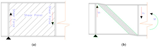
Figure 1.
Model of web in post-buckling range; (a) Shear force carried by web, (b) Shear force carried by truss action.
For the supposed failure mechanism, the ultimate shear resistance Vf. of a transversely stiffened girder can be expressed as:
The value of θ is governed by the panel aspect ratio (Cot θ = b/d).
A parametric study shows that the variation of Vult with θ is not abrupt [8,9]. An assumption of θ = 2 θd /3, in order to maximize where cot θd = b/d has been suggested [6]. BS 5950: Part 1 [44] provides a simplified version of the shear strength equations based on the assumption that θ = θd/2. The following formula can be presented based on the two critical phases of shear failure experienced in steel beams:
where is a factor that indicates the necessary adjustment for the value produced by the suggested formula and determined using Artificial Intelligence (AI).
4. Cascade forward Backpropagation
Artificial intelligence (AI) has become significant in the field of civil engineering, as it enables the rapid identification of mathematical models reflecting the participating physical models. In the civil engineering field [45,46], there are numerous applications, including smart sustainable buildings [47], overall construction, the purpose of the system, demolition of buildings, and construction-related durability [48,49]. A trainable cascade forward backpropagation network was used in this research. This is because, once a civil engineering technique has been chosen, it cannot be changed. As a result, it is critical to reconsider an earlier judgment [50]. A sensitivity analysis of the final decision is the most prevalent method utilized by decision-makers. Every failed operation requires shear stress, and it is vital to forecast shear stress for different beam shapes. Using cascade forward backpropagation neural networks, the purpose of this paper is to achieve consistency between experimental results and the suggested solution.
As shown in Figure 2, the cascade forward backpropagation model resembles feed-forward networks; however, although two-layer feed-forward networks can be utilized to analyze any input–output relationship, feed-forward networks with more layers can be utilized to examine the conflicting priorities quickly. The backpropagation method is applied for proportional improvement in the cascade forward backpropagation ANN model, which is like a feed-forward Backpropagation Neural Network. However, each layer of neurons in this network is related to the ones before it [51,52]. There are one or more interconnected hidden layers and activation functions in the Cascade-Forward Back-propagation Neural Network (CFBNN), as with other feed-forward networks. Neurons have biases of their own, and connections have normalized connections.
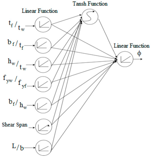
Figure 2.
Schematic of a trainable cascade-forward back-propagation ANN to determine the Shear Strength of Steel Beams.
Three weight matrices are employed to estimate output data in this ANN structure, the weight matrices between the input and hidden layers, the weight matrices between the input and output layers, and the weight matrices between the hidden and output layers. For the hidden and output layers, there are two bias matrices as well. The degree of freedom in this ANN structure is high [53,54,55,56]. Figure 3 depicts the learning process algorithm (2).
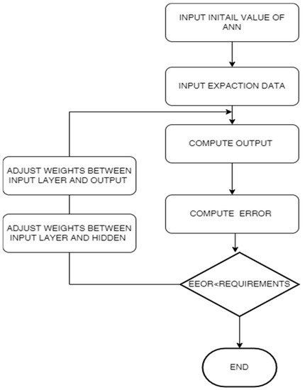
Figure 3.
Flowchart for the prediction method.
The following steps and Equations (21)–(27) illustrate the prediction of the shear strength of steel beams
Step 1: Nodes of the input layer receive data from the collected data. The input vector is IN,
IN = [tf/tw bf/tf hw/tw fyf/fyw bf/hw Shear Span L/bw]
Step 2: Output of the input layer passes to hidden nodes through the weighted links; the resulting weight matrix between the hidden and input neurons is given by (wih) and the hidden nodes biases are given by the bh.
Step 3: The output of hidden nodes results from the input signal passing through the activation function (tan-sigmoid function), the hidden layer output vector of ANN is oh, where
oh = tan − sig(wih × IN,bh)
Step 4: Output of the input layer passes to output nodes through the weighted links, the resulting weight matrix between the output and input neurons is given by wio and
oi = tan − sig(wio × IN)
Step 5: Hidden layer outputs are sent to the output nodes through weighted links; the resulting weight matrix between the hidden and output neurons is given by (who) and the hidden nodes biases are given by the bo.
Step 6: The ANN1 output is obtained using another activation function (Linear activation function); the output vector of ANN1 is o1, where
o1 = pure-lin (who × oh + oi, bo)
Step 7: The proposed cascade-forward back-propagation ANN to predict the yield of the Shear Strength of Steel Beams runs all the processes shown in Figure 2. This output function can be constructed in Microsoft Excel for the sequential solving of predicting Shear Strength problems. According to the proposed cascade-forward back-propagation mode,l which is described by the above equation, the investigated Solver in Excel has many advantages, such as it being a much simpler, intuitive, and easily available tool for the prediction of the shear strength of steel beams. In addition, the process of learning the mathematical model of this ANN can be described by the following equations
where the tf1 transfer function is a hyperbolic tangent sigmoid transfer and the tf2 and tf3 transfer functions are linear transfer functions. Table 2 shows the conversion from MATLAB to Microsoft Excel.
Table 2.
Converting from MATLAB to EXCEL.
The appropriate scaled root means square error percentage [nRMSE (percent)] is computed at different conditions to evaluate the accuracy of the proposed model, and it is matched to [nRMSE (percent)] of an accurate model. The normalized root means square error percentage [nRMSE (percent)] is presented in the following Equation (28).
The linear model has shown the best accuracy under many scenarios, where Ei is the estimation and Ti is the true values obtained from testing. Moreover, the degree of consistency and predictability has been reduced. The total number of samples is around 89 after the removal of the incomplete testing samples. The above equation yields the normalized root mean square error percentage [nRMSE (percent)], which is 0.5 percent [57,58]. The created model results for substituted in Equation (20) corresponding to each sample are shown in Table 3. The developed model for calculating is fully described in Appendix B, along with all the relations between it and the independent factors.
Table 3.
Sample results.
The results arising from the two European code cases and the suggested equation case are displayed in Table 3 together with their respective means and standard deviations. These numbers clearly demonstrate that the standard deviation of the suggested equation is 0.07, compared to a range of 0.2 to 0.19 for the European code. This shows the level of precision that the suggested equation can reach when estimating the maximum shear forces that the steel beams can withstand. According to the authors of [59], who evaluated the proposed ANN model with four notable current design code formulas, ANN models always demonstrate better accuracy than existing design code formulas as clearly confirmed by the obtained results in this study.
5. Appropriate Conditions for Using the Proposed Equation
The following conclusion can be reached based on the classification of flanges and webs and the seven different ratios used as input data for NI techniques shown in Appendix A. The outcomes of the suggested formula with the artificial intelligence-generated modification factor (Vprop) and a comparison of those outcomes with the experimental findings (Vexp) are displayed in Table 3. The proposed formula is dependent on four key variables, as shown in Table 4: (a) the ratio of flange to web thicknesses (tf/tw); (b) the ratio of flange width to web depth (bf/hw); (c) the ratio of transversal stiffener spacing to web depth (b/d); and (d) the ratio of load span to transversal stiffener spacing (L/b). These findings showed that more than 95% of the results obtained under these conditions matched the experimental shear strength reported in the literature
Table 4.
Limit state of the proposed equation.
6. Experimental Program
6.1. Specimen Details
Under three and four-point bending, two full-scale steel beams designated B1-3P as shown in Figure 4a,b where specimen B2-4P illustrated in Figure 4c,d were tested. In the two specimens, different shear spans and beam lengths were produced. The first specimen was made with greater shear spans and is subjected to three-point bending, whereas the second was made with shorter shear spans that are equal to the pure bending span. The first has a shear span of 900 mm and the second has a shear span of 800 mm. The height t of both specimens is 400 mm. Bearing stiffeners were attached to each specimen under the applied line load and supporting points.
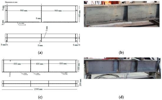
Figure 4.
Specimen dimensions and test setup: (a) B1-3P Specimen dimension; (b) B1-3P Specimen Setup; (c) B2-4P Specimen dimension; (d) B1-3P Specimen Setup.
The tested specimens had different total and effective spans. B1-3P and B2-4P have effective spans of 1800 mm and 2200 mm and total lengths of 1900 mm and 2300 mm, respectively. The web height (hw), web thickness (tw), flange breadth (bf), and flange thickness (tf) of all specimens were 384, 3, 200, and 8 mm, respectively. Thus, the determined height-to-thickness ratio (hw/tw) of the corrugated web for both specimens is 128. The compactness of the flanges for the experimentally investigated steel beams was assessed in terms of the outstanding length, i.e., (bf-tw)/2tf = 12.31. Depending on the web and flange slenderness ratios, the section might be classed as non-compact flange and slender web according to EC3 [8].
6.2. Specimen Materials Properties
In this study, the steel mechanical characteristics for the structural tested beams were obtained through the testing of six standard specimens in tension. The tension specimens were cut from the web and flanges (three from each part). The specimens were cut far away from the flame-cut side and adopted to the nearest 0.01 mm, and then examined in accordance with EN 10002-1 standard. A 2000-kN strength displacement-self-controlled testing machine was used to apply tension loads to the tested specimens. The Young’s modulus, the tensile strength tensile strain, and yield strength (fy) obtained from these tests are described as scheduled in Table 5.
Table 5.
Modulus of elasticity, maximum strain, and ultimate and yield stresses.
6.3. Test Procedure and Results
A concentrated line load was applied to the experimented beams at their center line with an increment of 55.55 N/sec. The un-braced length of the compressive flanges was 1800 mm for the experimented beams (the supports spacing distance). Table 6 shows the load capacities, corresponding deflection, and failure mechanisms of the tested specimens. The behavior of the tested specimens in terms of stiffness, buckling, and failure mode mechanism based on the number of point load testing results and test observations are shown in Table 6 and Figure 5.
Table 6.
Specimen test results.
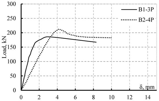
Figure 5.
Load deflection curves for specimens B1-3P and B2-4P.
Both specimens B1-3P and B2-4P failed due to global web buckling at loads of 188 and 212 kN, respectively, as illustrated in Figure 5. Figure 5 shows the mid-span vertical displacements of the test specimens. By comparing the behavior of specimen B1-3P with specimen B2-4P, it is noticed that specimen B1-3P exhibited a high initial stiffness but low ultimate strength and vertical deflection due to the fact of span and loading conditions.
The results reveal that the flange of specimens B1-3P and B2-4P remained undamaged through the test until the ending the test. The experiments conducted by the authors revealed that the collapse of steel beams exposed to bending and shear was controlled by the web stress at the maximum shear sections as expected. Figure 6 also reveals a comparison of the web buckling angles of the B1-3P and B2-4P beams.
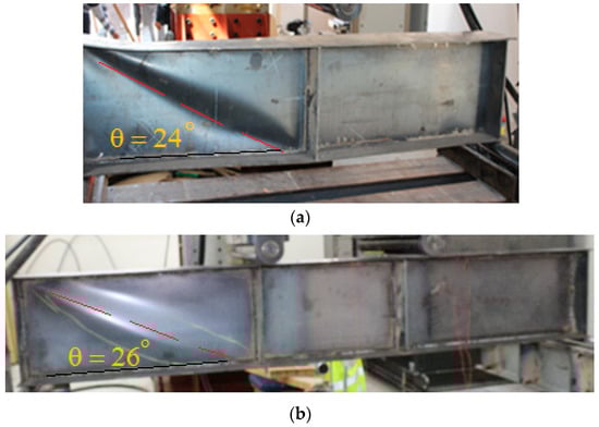
Figure 6.
Failure mode and angle–(a) Specimen B1-3P (b) Specimen B2-4P.
These findings corroborate the efficiency of the vertical stiffeners for raising the beam shear resistance and postponing web buckling. The specimens B1-3P and B2-4P failed due to web buckling running between the two corners that are neither loaded nor supported as shown in Figure 6. Figure 6 also shows the web-buckling angle of specimens B1-3P and B2-4P, which are almost 24 and 26 degrees, respectively. The maximum vertical deflection value (δ) achieved at load capacities of B1-3P and B2-4P were 8.3 and 10 mm, respectively, corresponding to the stage where the actuator is automatically stopped.
7. Verification of Proposed Formula
The authors’ experimental program results and the findings of Roberts and Shahabian’s [60] experimental work are used to verify the suggested formula with the factor produced by ANN. Table 7 lists the dimensions and material characteristics of the four specimens that were put through an experimental shear load test by [60].
Table 7.
Specimen details and test results [60].
The limit state of each specimen either tested by the authors or by Roberts and Shahabian in [60] is shown in Table 8.
Table 8.
Classification of verification samples according to limit state.
Table 9 displays the results of the suggested equation for shear strength and the correction factor obtained from the ANN formula. The final shear strengths obtained for each specimen in the experiments conducted by the authors or reported by [60] are compared to the predicted values computed using Equation (20). Equation (20) uses the inverse of the value derived from the AI model for each specimen as the 1/ factor.
Table 9.
Verification results.
8. Conclusions
In this study, a novel method for estimating the maximum shear strength of steel beams with a flat web was presented. An artificial intelligence (AI)-based strategy was applied. The study began by gathering data from earlier experimental work, followed by the proposal of a new equation and the use of AI to develop a modified factor, followed by two alternative methods of verification. The 96 test results of various specimen parameters gathered from previous work served as the foundation for the model. The model requires seven different ratios as input data, as given in Appendix A. According to the study, the suggested equations with the modification factor may predict the steel beam’s shear strength with a respectable level of accuracy. To obtain results from the suggested equation, the following constraints have to be taken into consideration:
- An acceptable level of accuracy can be achieved in predicting the final shear force using the proposed equation.
- When compact flanges and a slender web are paired, accurate results can be achieved if the flange width to web depth ratio is less than or equal to 0.33.
- For compact flanges and non-compact webs, the optimum quantitative relationship between the two thicknesses is less than or equal to 6.5, which allows for the prediction of the nearest achievable shear strength.
- In the case of non-compact flanges and a slender web, it is advisable to have one of the following two conditions; (a) the ratio of the transversal stiffener spacing to web depth (b/d) should be less than or equal to 1 when the load span to stiffener spacing (L/b) is more than or equal to 2; or (b) the ratio of b/d should be less than or equal to 2.5 when L/b is equal to 1.
- In the majority of classification cases, the ratio of transverse stiffener spacing to web height is the main variable that has a substantial impact on the accuracy of the modified factor results.
Author Contributions
Methodology, A.S.E., A.K.M. and Y.M.A.; Software, M.A.M.A.; Validation, I.A.S.; Formal analysis, A.S.E., M.A.M.A. and M.A.M.; Investigation, I.A.S. and A.K.M.; Data curation, A.S.E.; Writing – original draft, I.A.S. and M.A.M.; Project administration, Y.M.A.; Funding acquisition, Y.M.A. All authors have read and agreed to the published version of the manuscript.
Funding
This research was funded by the Taif University Researchers grant number TURSP-2020/276.
Institutional Review Board Statement
Not applicable.
Informed Consent Statement
Not applicable.
Data Availability Statement
The datasets used and/or analyzed are available from the corresponding author on reasonable request.
Acknowledgments
This work was supported by the Taif University Researchers Supporting Project Number (TURSP-2020/276), Taif University, Taif, Saudi Arabia. The funding source was not involved in the study design; in the collection, analysis, and interpretation of data; in the writing of the report; or in the decision to submit the article for publication.
Conflicts of Interest
The authors do not have any conflicts of interest to declare.
Appendix A. Classification of Web and Flange
| Sep No. | tf/tw | bf/2tf | hw/tw | fyw/fyf | bf/hw | b/d | L/b | Web | Flange | |
| C4 | [19] | 4.35 | 3.20 | 242.18 | 0.90 | 0.12 | 0.71 | 2.00 | Slender | Compact |
| G6-T1 | [20] | 4.04 | 7.78 | 259.18 | 0.97 | 0.24 | 1.50 | 1.00 | Slender | Compact |
| G6-T2 | 4.04 | 7.78 | 259.18 | 0.97 | 0.24 | 0.75 | 2.00 | Slender | Compact | |
| G6-T3 | 4.04 | 7.78 | 259.18 | 0.97 | 0.24 | 0.50 | 3.00 | Slender | Compact | |
| G7-T1 | 3.92 | 7.95 | 255.02 | 0.98 | 0.24 | 1.00 | 1.50 | Slender | Compact | |
| G7-T2 | 3.92 | 7.95 | 255.02 | 0.98 | 0.24 | 1.00 | 1.50 | Slender | Compact | |
| G8-T1 | 3.76 | 7.98 | 250.00 | 0.93 | 0.24 | 3.00 | 1.00 | Slender | Compact | |
| G8-T2 | 3.76 | 7.98 | 250.00 | 0.93 | 0.24 | 1.50 | 1.00 | Slender | Compact | |
| G8-T3 | 3.76 | 7.98 | 250.00 | 0.93 | 0.24 | 1.50 | 2.00 | Slender | Compact | |
| G9-T1 | 5.74 | 7.98 | 381.38 | 1.07 | 0.24 | 3.00 | 1.00 | Slender | Compact | |
| G9-T2 | 5.74 | 7.98 | 381.38 | 1.07 | 0.24 | 1.50 | 1.00 | Slender | Compact | |
| G9-T3 | 5.74 | 7.98 | 381.38 | 1.07 | 0.24 | 1.50 | 2.00 | Slender | Compact | |
| E1T2 | [21] | 2.48 | 9.25 | 127.25 | 1.06 | 0.36 | 1.50 | 1.00 | Slender | Non-Compact |
| E2T1 | 5.17 | 4.48 | 128.15 | 1.01 | 0.36 | 1.00 | 3.00 | Slender | Compact | |
| C-AC2 | [22] | 3.03 | 5.43 | 147.48 | 0.28 | 0.22 | 5.45 | 1.00 | Non-Compact | Compact |
| C-AC4 | 3.98 | 3.90 | 111.51 | 0.30 | 0.28 | 5.50 | 1.00 | Compact | Compact | |
| C-AC5 | 4.44 | 3.32 | 106.33 | 0.30 | 0.28 | 5.50 | 1.00 | Compact | Compact | |
| B | [23] | 2.67 | 10.00 | 266.67 | 1.00 | 0.20 | 1.00 | 1.00 | Slender | Non-Compact |
| 3-2 | [24] | 3.28 | 4.76 | 99.69 | 1.29 | 0.31 | 1.82 | 1.00 | Non-Compact | Compact |
| 3-3 | 3.28 | 4.81 | 149.06 | 1.17 | 0.21 | 1.21 | 1.00 | Slender | Compact | |
| 2·2 | [25] | 3.00 | 14.58 | 300.00 | 1.00 | 0.29 | 2.40 | 1.00 | Slender | Non-Compact |
| TG3 | [26] | 6.56 | 6.10 | 400.00 | 0.71 | 0.20 | 1.00 | 1.00 | Slender | Compact |
| TG3-1 | 6.56 | 6.10 | 400.00 | 0.71 | 0.20 | 1.00 | 1.00 | Slender | Compact | |
| TG4 | 8.08 | 4.95 | 400.00 | 0.71 | 0.20 | 1.00 | 1.00 | Slender | Compact | |
| TG4-1 | 8.04 | 4.98 | 400.00 | 0.71 | 0.20 | 1.00 | 1.00 | Slender | Compact | |
| TG5 | 11.88 | 3.37 | 400.00 | 0.71 | 0.20 | 1.00 | 1.00 | Slender | Compact | |
| TG5-1 | 11.88 | 3.37 | 400.00 | 0.71 | 0.20 | 1.00 | 1.00 | Slender | Compact | |
| U32/5 | [27] | 3.79 | 4.04 | 113.25 | 0.55 | 0.27 | 2.19 | 1.55 | Compact | Compact |
| U33/5 | 4.44 | 4.00 | 132.96 | 0.61 | 0.27 | 2.19 | 2.06 | Non-Compact | Compact | |
| TG14 | [28] | 3.22 | 12.18 | 314.43 | 0.72 | 0.25 | 1.00 | 2.00 | Slender | Non-Compact |
| TG15 | 5.15 | 7.60 | 314.43 | 0.77 | 0.25 | 1.00 | 2.00 | Slender | Compact | |
| TG16 | 6.65 | 5.89 | 314.43 | 0.65 | 0.25 | 1.00 | 2.00 | Slender | Compact | |
| TG17 | 9.61 | 4.08 | 314.43 | 0.71 | 0.25 | 1.00 | 2.00 | Slender | Compact | |
| TG18 | 13.40 | 2.92 | 314.43 | 0.72 | 0.25 | 1.00 | 2.00 | Slender | Compact | |
| TG19 | 15.98 | 2.45 | 314.43 | 0.82 | 0.25 | 1.00 | 2.00 | Slender | Compact | |
| TG22 | 3.20 | 5.85 | 150.25 | 0.68 | 0.25 | 1.00 | 2.00 | Non-Compact | Compact | |
| TG23 | 4.53 | 4.13 | 150.25 | 0.74 | 0.25 | 1.00 | 2.00 | Non-Compact | Compact | |
| TG24 | 6.40 | 2.92 | 150.25 | 0.75 | 0.25 | 1.00 | 2.00 | Non-Compact | Compact | |
| TG25 | 7.64 | 2.45 | 150.25 | 0.85 | 0.25 | 1.00 | 2.00 | Non-Compact | Compact | |
| 3TG1 | 3.95 | 8.04 | 139.50 | 0.93 | 0.46 | 1.97 | 1.00 | Non-Compact | Compact | |
| 3TG2 | 4.00 | 9.92 | 158.13 | 0.99 | 0.50 | 1.98 | 1.00 | Non-Compact | Compact | |
| 3TG4 | 5.12 | 7.97 | 200.80 | 0.89 | 0.41 | 1.98 | 1.00 | Slender | Compact | |
| RTG1 | 3.54 | 8.44 | 240.16 | 0.89 | 0.25 | 1.00 | 2.00 | Slender | Compact | |
| RTG2 | 3.70 | 8.09 | 240.16 | 0.89 | 0.25 | 1.00 | 2.00 | Slender | Compact | |
| RTG4 | 4.95 | 8.09 | 267.37 | 0.94 | 0.30 | 1.00 | 2.00 | Slender | Compact | |
| T31/3 | [29] | 2.96 | 8.71 | 200.25 | 0.62 | 0.26 | 0.86 | 4.06 | Slender | Non-Compact |
| T31/4 | 2.96 | 8.83 | 200.25 | 0.62 | 0.26 | 0.86 | 2.00 | Slender | Non-Compact | |
| M3O | [30] | 5.02 | 5.05 | 302.49 | 0.97 | 0.17 | 1.56 | 1.00 | Slender | Compact |
| 3D1 | [31] | 6.00 | 10.42 | 297.00 | 1.30 | 0.42 | 1.00 | 4.49 | Slender | Compact |
| 3D3 | 6.00 | 10.42 | 297.00 | 1.30 | 0.42 | 1.00 | 1.80 | Slender | Compact | |
| TGV1-1 | [32] | 4.83 | 10.00 | 289.86 | 0.85 | 0.33 | 2.00 | 1.00 | Slender | Compact |
| TGV1-2 | 4.83 | 10.00 | 289.86 | 0.85 | 0.33 | 1.00 | 2.00 | Slender | Compact | |
| TGV2-2 | 4.81 | 10.00 | 288.46 | 0.85 | 0.33 | 1.00 | 2.00 | Slender | Compact | |
| TGV3-2 | 4.98 | 10.00 | 298.51 | 0.85 | 0.33 | 1.00 | 2.00 | Slender | Compact | |
| TGV4 | 5.13 | 9.95 | 303.55 | 0.88 | 0.34 | 1.00 | 2.00 | Slender | Compact | |
| TGV5 | 5.05 | 10.05 | 302.02 | 0.92 | 0.34 | 0.99 | 2.00 | Slender | Compact | |
| TGV6 | 5.13 | 9.95 | 303.55 | 0.90 | 0.34 | 0.99 | 2.00 | Slender | Compact | |
| TGV7-2 | 5.10 | 9.95 | 302.53 | 0.88 | 0.34 | 0.99 | 2.00 | Slender | Compact | |
| TGV10-1 | 5.24 | 10.00 | 313.61 | 0.77 | 0.33 | 0.99 | 2.00 | Slender | Compact | |
| TGV10-2 | 5.24 | 10.00 | 313.61 | 0.77 | 0.33 | 0.99 | 2.00 | Slender | Compact | |
| TGV11-2 | 5.24 | 10.00 | 313.61 | 1.04 | 0.33 | 1.00 | 2.00 | Slender | Compact | |
| 33/1 | [33] | 3.11 | 5.47 | 291.26 | 0.57 | 0.12 | 1.00 | 1.00 | Slender | Compact |
| 34/1 | 2.99 | 6.25 | 328.04 | 0.57 | 0.11 | 0.98 | 1.00 | Slender | Compact | |
| 35/1 | 2.94 | 6.09 | 366.06 | 0.57 | 0.10 | 1.00 | 1.00 | Slender | Compact | |
| 32/1·5 | 3.05 | 6.25 | 237.14 | 0.57 | 0.16 | 1.51 | 1.00 | Slender | Compact | |
| 33/1·5 | 3.11 | 6.09 | 292.23 | 0.57 | 0.13 | 1.50 | 1.00 | Slender | Compact | |
| 34/1·5 | 3.00 | 5.91 | 320.00 | 0.57 | 0.11 | 1.48 | 1.00 | Slender | Compact | |
| L31-PA | [34] | 4.76 | 5.00 | 289.52 | 0.68 | 0.16 | 1.55 | 1.00 | Slender | Compact |
| L33-PA | 4.11 | 4.95 | 247.15 | 0.71 | 0.16 | 1.56 | 1.00 | Slender | Compact | |
| MC31-PB3 | [35] | 3.43 | 9.93 | 227.27 | 0.75 | 0.30 | 0.73 | 2.00 | Slender | Compact |
| PA1 | [36] | 12.00 | 10.38 | 800.00 | 1.05 | 0.31 | 0.75 | 5.00 | Slender | Compact |
| PA2 | 12.00 | 10.38 | 800.00 | 1.05 | 0.31 | 0.75 | 4.00 | Slender | Compact | |
| PA3 | 12.00 | 10.38 | 800.00 | 1.05 | 0.31 | 0.75 | 3.00 | Slender | Compact | |
| PB1 | 12.00 | 10.38 | 800.00 | 1.05 | 0.31 | 0.63 | 6.00 | Slender | Compact | |
| PB2 | 12.00 | 10.38 | 800.00 | 1.05 | 0.31 | 0.63 | 5.00 | Slender | Compact | |
| PC1 | 10.00 | 12.50 | 800.00 | 0.82 | 0.31 | 1.25 | 2.75 | Slender | Non-Compact | |
| PC2 | 10.00 | 12.50 | 800.00 | 0.82 | 0.31 | 1.25 | 1.75 | Slender | Non-Compact | |
| PD1 | 10.00 | 12.50 | 800.00 | 0.82 | 0.31 | 0.94 | 3.67 | Slender | Non-Compact | |
| PD2 | 10.00 | 12.50 | 800.00 | 0.82 | 0.31 | 0.94 | 2.67 | Slender | Non-Compact | |
| PD3 | 10.00 | 12.50 | 800.00 | 0.82 | 0.31 | 0.94 | 1.67 | Slender | Non-Compact | |
| PC3 | 10.00 | 12.50 | 800.00 | 0.82 | 0.31 | 0.94 | 1.00 | Slender | Non-Compact | |
| PB3 | [37] | 3.43 | 9.93 | 227.27 | 0.75 | 0.30 | 0.73 | 2.00 | Slender | Compact |
| PB4 | 3.43 | 9.93 | 227.27 | 0.75 | 0.30 | 0.73 | 2.00 | Slender | Compact | |
| B1 | [38] | 3.46 | 11.41 | 209.79 | 1.43 | 0.38 | 15.00 | 1.00 | Slender | Non-Compact |
| B4 | 3.05 | 12.38 | 300.00 | 0.92 | 0.25 | 15.00 | 1.00 | Slender | Non-Compact | |
| K1 | 3.46 | 11.41 | 209.79 | 1.43 | 0.38 | 10.00 | 1.00 | Slender | Non-Compact | |
| 1A | [39] | 3.38 | 11.25 | 202.70 | 0.97 | 0.38 | 13.50 | 1.00 | Slender | Non-Compact |
| 1B | 3.37 | 11.25 | 202.02 | 0.97 | 0.38 | 13.50 | 1.00 | Slender | Non-Compact | |
| 2A | 3.33 | 11.25 | 200.00 | 0.97 | 0.38 | 13.50 | 1.00 | Slender | Non-Compact | |
| 2B | 3.40 | 11.25 | 204.08 | 0.97 | 0.38 | 13.50 | 1.00 | Slender | Non-Compact | |
| 3A | 3.00 | 12.50 | 300.00 | 1.02 | 0.25 | 13.50 | 1.00 | Slender | Non-Compact | |
| 3B | 3.00 | 12.50 | 300.00 | 1.02 | 0.25 | 13.50 | 1.00 | Slender | Non-Compact | |
| 4A | 2.99 | 12.50 | 298.51 | 1.02 | 0.25 | 13.50 | 1.00 | Slender | Non-Compact | |
| 4B | 2.96 | 12.50 | 295.57 | 1.02 | 0.25 | 13.50 | 1.00 | Slender | Non-Compact | |
| CP1/1 | [40] | 3.92 | 6.25 | 245.10 | 0.96 | 0.20 | 1.49 | 1.00 | Slender | Compact |
| RCP1/1 | [41] | 4.03 | 6.17 | 357.21 | 0.94 | 0.14 | 0.99 | 1.00 | Slender | Compact |
Appendix B
[(33954415511283800*)/103512422685343000 − (28442070878220100*)/28112313298976700 + (282414137877243**)/9007199254740990 + (101297774103200000*)/322007373356990000 + (1374602471662690*)/70368744177664 − (8440126075848900*)/16888498602639300 − (7340558476484290*)/54043195528445900] + [212475039604665/(549755813888*(EXP((2373031373901580**)/900719925474099000 − (63347333402543200*)/828099381482749000 − (28149491545881100*)/28112313298976700 + (64705199509204500*)/40250921669623800 + (6442135245746950**)/2251799813685240 − (8885013206467490*)/67553994410557400 − (1296189573031780**)/27021597764222900 + 8253290674290910/1125899906842620) + 1))] – [6823642198234820/(17592186044416*(EXP((1179756069166860**)/450359962737049000 − (133923952776203000*)/1656198762965490000 − (112830641941746000*)/112449253195907000 + (62420121156409000*)/40250921669623800 + (7940027530145260**)/2251799813685240 − (366224999899617*)/2814749767106560 − (2358086171817460**)/72057594037927900 + 4069325028141150/562949953421312) + 1)) ] – [1604169459141280/(140737488355328*(EXP((125241952769013000*)/899594025567256000 − (113139814729844000*)/414049690741374000 − (488928742597863**)/90071992547409900 + (194101123417720000*)/10304235947423600000 − (6241223000095810**)/1125899906842620 + (7429000628497040*)/67553994410557400 + (420111069608599**)/13510798882111400 + 6103890632617880/2251799813685240) + 1)) ] + [7630333641755660/(2251799813685240*(EXP((51610101196082900*)/103512422685343000 − (119366504384797000*)/112449253195907000 − (3074933687020290*)/112589990684262000 + (10372280686951400*)/7318349394477050 + (4777270297371930**)/70368744177664 + (2303030245661500*)/5629499534213120 + (680529090821275**)/844424930131968 + 7720690751003840/72057594037927900) + 1))] – [7798682056076260/(17592186044416*(EXP((76097331593009600*)/224898506391814000 + (98774818315865900*)/207024845370687000 − (3067421494356520**)/450359962737049000 + (117694759407178000*)/10304235947423600000 − (3832512185894430**)/2251799813685240 + (1695379762604800*)/45035996273704900 + (5501779190389850**)/27021597764222900 − 5710765195203270/1125899906842620) + 1))] – [1960416135087140/(4398046511104*(EXP((1501074293996440**)/225179981368524000 − (198604442843452000*)/414049690741374000 − (151517583083059000*)/449797012783628000 − (158024583342534000*)/20608471894847300000 + (3606233885717940**)/2251799813685240 − (2331482887278890*)/67553994410557400 − (1813943982980590**)/9007199254740990 + 5802006042731420/1125899906842620) + 1))] – [2496368182043530/(281474976710656*(EXP((54312850784934900*)/56224626597953500 + (83188269152295200*)/207024845370687000 − (2690522990955420**)/112589990684262000 + (15350383231948500*)/117093590311632000 − (7437737313840860**)/2251799813685240 + (5964446694710020*)/8444249301319680 − (4228311206345060**)/13510798882111400 + 7784845848360150/2251799813685240) + 1)) + 1991369913313520000/4503599627370490].
References
- Davies, A.W.; Griffith, D.S. Shear Strength of steel plate girder. Proc. Inst. Civ. Eng.-Struct. Build. 1999, 134, 147–157. [Google Scholar] [CrossRef]
- Sulyok, M.; Galambos, T.V. Evaluation of web buckling test results on welded beams and plate girders subjected to shear. Eng. Struct. 1996, 18, 459–464. [Google Scholar] [CrossRef]
- Lee, S.C.; Davidson, J.S.; Yoo, C.H. Shear buckling coefficients of plate girder web panels. Comput. Struct. 1996, 59, 789–795. [Google Scholar] [CrossRef]
- Lee, S.C.; Yoo, C.H. Strength of Plate Girder Web Panels under Pure Shear. J. Struct. Eng. 1998, 124, 184–194. [Google Scholar] [CrossRef]
- Shahabian, F.; Roberts, T.M. Combined Shear-and-Patch Loading of Plate Girders. J. Struct. Eng. 2000, 126, 316–321. [Google Scholar] [CrossRef]
- Bradford, M.A. Improved Shear Strength of Webs Designed in Accordance with the LRFD Specification. Eng. J. 1996, 33, 95–100. [Google Scholar]
- Höglund, T. Shear buckling resistance of steel and aluminium plate girders. Thin-Walled Struct. 1997, 29, 13–30. [Google Scholar] [CrossRef]
- ENV 1993-1-3 Eurocode 3: Design of steel structures: Part 1.1. In General Rules and Rules for Buildings; BSI: Afghanistan, Middle East, 1992.
- Nethercot, D.A.; Byfield, M.P. Calibration of Design Procedures for Steel Plate Girders. Adv. Struct. Eng. 1997, 1, 111–126. [Google Scholar] [CrossRef]
- Barakat, S.; Mansouri, A.A.; Altoubat, S. Shear strength of steel beams with trapezoidal corrugated webs using regression analysis. Steel Compos. Struct. 2015, 18, 757–773. [Google Scholar] [CrossRef]
- Elamary, A.S.; Taha, I.B.M. Determining the Shear Capacity of Steel Beams with Corrugated Webs by Using Optimised Regression Learner Techniques. Materials 2021, 14, 2364. [Google Scholar] [CrossRef]
- Ben Seghier, M.E.A.; Ouaer, H.; Ghriga, M.A.; Menad, N.A.; Thai, D.-K. Hybrid soft computational approaches for modeling the maximum ultimate bond strength between the corroded steel reinforcement and surrounding concrete. Neural Comput. Appl. 2021, 33, 6905–6920. [Google Scholar] [CrossRef]
- Seghier, M.E.; Plevris, V.; Solorzano, G. Random forest-based algorithms for accurate evaluation of ultimate bending capacity of steel tubes. Structures 2022, 44, 261–273. [Google Scholar] [CrossRef]
- Khalaj, G.; Azimzadegan, T.; Khoeini, M.; Etaat, M. Artificial neural networks application to predict the ultimate tensile strength of X70 pipeline steels. Neural Comput. Appl. 2013, 23, 2301–2308. [Google Scholar] [CrossRef]
- Khalaj, G.; Pouraliakbar, H.; Mamaghani, K.R.; Khalaj, M.J. Modeling the correlation between heat treatment, chemical composition and bainite fraction of pipeline steels by means of artificial neural networks. Neural Netw. World 2013, 23, 351. [Google Scholar] [CrossRef]
- ELamary, A.S. Cardiff theory: Web panel aspect ratio limits and their relation with inclination angle of membrane tensile yield strength. Int. J. Steel Struct. 2016, 16, 799–806. [Google Scholar] [CrossRef]
- ELamary, A.S. Ultimate shear strength of composite welded steel-aluminium beam subjected to shear load. Int. J. Steel Struct. 2016, 16, 41–50. [Google Scholar] [CrossRef]
- Lee, S.C.; Lee, D.S.; Yoo, C.H. Ultimate shear strength of long web panels. J. Constr. Steel Res. 2008, 64, 1357–1365. [Google Scholar] [CrossRef]
- Longbottom, E.; Heymay, J. Experimental verification of the strength of plate girders designed in accordance with the revised British Standard 153: Tests on full scale model plate girders. Proc. Inst. Civ. Eng. 1956, 5, 462–486. [Google Scholar] [CrossRef]
- Basler, K.; Yen, B.-T.; Mueller, J.A.; Thürlimann, B. Web buckling tests on welded plate girders, Part 3: Tests on plate girders subjected to shear. Welded Plate Girder Proj. Comm. 1960, 165, 48. [Google Scholar]
- Cooper, P.B.; Lew, H.S.; Yen, B.T. Welded constructional alloy steel plate girders. J. Struct. Div. 1964, 90, 1–36. [Google Scholar] [CrossRef]
- Carskaddan, P.S. Shear buckling of unstiffened hybrid beams. J. Struct. Div. 1968, 94, 1965–1990. [Google Scholar] [CrossRef]
- Konishi, I. Theory and Experiment of Load Carrying Capacity of Plate Girders; Research Committee: Kansai District, Japan, 1965. [Google Scholar]
- Sakai, F.; Fujii, T.; Fukucei, Y. Failure Tests of Plate Girders Using Large-Sided Models; University of Tokyo: Tokyo, Japan, 1966. [Google Scholar]
- Bergfelt, A.; Hövik, J. Thin-walled deep plate girders under static loads. In Proceedings of the IABSE Colloquium; New York. 1968. Available online: https://www.e-periodica.ch/cntmng?pid=bse-cr-001:1968:8::132 (accessed on 5 November 2022).
- Skaloud, M. Ultimate load and failure mechanism of thin webs in shear. In Design of Plate and Box Girders for Ultimate Strength Colloquium; IABSE: London, UK, 1971. [Google Scholar]
- Kamtekar, A.G.; Dwiget, J.B.; Terelfall, B.D. Tests on Hybrid Plate Girders (Report 2). Cambridge University, Report No. CUED/C-Struct/TR28 Cambridge, 1972.
- Rockey, K.C.; Skaloud, M. The ultimate load behavior of plate girders loaded in shear. Struct. Eng. 1972, 1, 29–48. [Google Scholar]
- Kamtekar, A.G.; Dwiget, J.B.; Terelfall, B.D. Tests on Hybrid Plate Girders (Report 3). Cambridge, 1974.
- Evans, H.R.; Rockey, K.C.; Porter, D.M. Tests on longitudinally reinforced plate girders subjected to shear. In Proceedings of the Conference of Structural Stability; Preliminary Report; Structural Stability Research Council (SSRC): Liege, Belgium, 1977; pp. 295–304. [Google Scholar]
- Evans, E.R.; Rockey, K.C.; Tang, K.H. An investigation into the Rigidity of Longitudinal Web Stiffeners for Plate Girders; University of wales, College of Cardiff, 1979. [Google Scholar]
- Rockey, K.C.; Valtinat, G.; Tang, K.H. The design of transverse stiffeners on webs loaded in shear—An ultimate load approach. Proc. Inst. Civ. Eng. 1981, 71, 1069–1099. [Google Scholar] [CrossRef]
- Adorisio, D. Model Studies on Plate Girders Subject to Shear Loading; University of Wales: Cardiff, UK, 1982. [Google Scholar]
- Evans, H.R.; Tang, K.H. An Investigation of the Ultimate Load Behavior of Longitudinally Stiffened Plate Girder Webs Loaded Predominantly in Shear. 1983.
- Evans, H.R. A Report on the Full Scale Tests on a Girder with a Stiffened Web Subjected to Combined Shear and Bending Loads; University of Wales College of Cardiff: Cardiff, UK, 1984. [Google Scholar]
- Tang, K.H.; Evans, H.R. Transverse stiffeners for plate girder webs—An experimental study. J. Constr. Steel Res. 1984, 4, 253–280. [Google Scholar] [CrossRef]
- Evans, H.R. An appraisal, by full scale testing, of new design procedures for steel girders subjected to shear and bending. Proc. Inst. Civ. Eng. 1986, 81, 175–189. [Google Scholar] [CrossRef]
- Leiva, L. Shear Buckling of Trapezoidally Corrugated Girder Webs; Report 583:3, Part 2; Chalmers University of Technology, Division of Steel and Timber Structures: Goteborg, Sweden, 1983. [Google Scholar]
- Frey, F.; Anslijn, R. Shear tests on unstiffened plate girders. In Proceedings of the Second International Colloquium on the Stability of Steel Structures, ECC3, 13–15 April 1977, Liege, Belgium; pp. 321–326.
- Narayanan, R.; Rockey, K.C. Ultimate load capacity of plate girders with webs containing circular cut-outs. Proc. Inst. Civ. Eng. 1981, 71, 845–862. [Google Scholar] [CrossRef]
- Der Avanessian, N.G.V. Ultimate Strength of Plate Girders Containing openings in Webs; University of Wales: Cardiff, UK, 1983. [Google Scholar]
- Porter, D.M.; Rockey, K.C.; Evan, E.R. The collapse behaviour of plate girders loaded in shear. Struct. Eng. 1975, 53, 313–325. [Google Scholar]
- Evans, H.R. Longitudinally and transversely reinforced plate girders." Plated Structures. In Stability and Strength; Narayanan, R., Ed.; Elsevier, Applied Science: London, UK, 1983; pp. 1–37. [Google Scholar]
- BS 5950; Part 1. Structural Use of Steel work in Building. Code of Practice for Design–Rolled and Welded Sections. British Standards Institution: London, UK, 2000; Volume 1, ISBN 9781859421796.
- Manzoor, B.; Othman, I.; Durdyev, S.; Ismail, S.; Wahab, M. Influence of Artificial Intelligence in Civil Engineering toward Sustainable Development—A Systematic Literature Review. Appl. Syst. Innov. 2021, 4, 52. [Google Scholar] [CrossRef]
- Gomes Correia, A.; Cortez, P.; Tinoco, J.; Marques, R. Artificial Intelligence Applications in Transportation Geotechnics. Geotech. Geol. Eng. 2013, 31, 861–879. [Google Scholar] [CrossRef]
- Luckey, D.; Fritz, H.; Legatiuk, D.; Dragos, K.; Smarsly, K. Artificial intelligence techniques for smart city applications. In International Conference on Computing in Civil and Building Engineering; Springer: New York, NY, USA; Sao Paulo, Brazil, 2020; pp. 3–15. [Google Scholar]
- Tavana Amlashi, A.; Alidoust, P.; Pazhouhi, M.; Pourrostami Niavol, K.; Khabiri, S.; Ghanizadeh, A.R. AI-Based Formulation for Mechanical and Workability Properties of Eco-Friendly Concrete Made by Waste Foundry Sand. J. Mater. Civ. Eng. 2021, 33, 04021038. [Google Scholar] [CrossRef]
- Zavadskas, E.; Antucheviciene, J.; Vilutiene, T.; Adeli, H. Sustainable Decision-Making in Civil Engineering, Construction and Building Technology. Sustainability 2017, 10, 14. [Google Scholar] [CrossRef]
- Luciano, A.; Cutaia, L.; Cioffi, F.; Sinibaldi, C. Demolition and construction recycling unified management: The DECORUM platform for improvement of resource efficiency in the construction sector. Environ. Sci. Pollut. Res. 2021, 28, 24558–24569. [Google Scholar] [CrossRef] [PubMed]
- Yaseen, Z.M.; Ali, Z.H.; Salih, S.Q.; Al-Ansari, N. Prediction of Risk Delay in Construction Projects Using a Hybrid Artificial Intelligence Model. Sustainability 2020, 12, 1514. [Google Scholar] [CrossRef]
- Shohda, A.M.A.; Ali, M.A.M.; Ren, G.; Kim, J.-G.; Mohamed, M.A.-E.-H. Application of Cascade Forward Backpropagation Neural Networks for Selecting Mining Methods. Sustainability 2022, 14, 635. [Google Scholar] [CrossRef]
- Basaran, U.B.; Kurban, M. A New Approach for the Short-Term Load Forecasting with Autoregressive and Artificial Neural Network Models. Int. J. Comput. Intell. Res. 2007, 3, 66–71. [Google Scholar] [CrossRef]
- Jha, K.; Doshi, A.; Patel, P.; Shah, M. A comprehensive review on automation in agriculture using artificial intelligence. Artificial Intelligence in Agriculture 2019, 2, 1–12. [Google Scholar] [CrossRef]
- Soofastaei, A. The Application of Artificial Intelligence to Reduce Greenhouse Gas Emissions in the Mining Industry. In Green Technologies to Improve the Environment on Earth; IntechOpen: London, UK, 2019. [Google Scholar]
- Mahmoud Ali, M.; Omran, A.N.M.; Abd-El-Hakeem Mohamed, M. Prediction the correlations between hardness and tensile properties of aluminium-silicon alloys produced by various modifiers and grain refineries using regression analysis and an artificial neural network model. Eng. Sci. Technol. Int. J. 2021, 24, 105–111. [Google Scholar] [CrossRef]
- Chai, T.; Draxler, R.R. Root mean square error (RMSE) or mean absolute error (MAE)?—Arguments against avoiding RMSE in the literature. Geosci. Model Dev. 2014, 7, 1247–1250. [Google Scholar] [CrossRef]
- Willmott, C.; Matsuura, K. Advantages of the mean absolute error (MAE) over the root mean square error (RMSE) in assessing average model performance. Clim. Res. 2005, 30, 79–82. [Google Scholar] [CrossRef]
- Tran, V.-L.; Thai, D.-K.; Nguyen, D.-D. Practical artificial neural network tool for predicting the axial compression capacity of circular concrete-filled steel tube columns with ultra-high-strength concrete. Thin-Walled Struct. 2020, 151, 106720. [Google Scholar] [CrossRef]
- Roberts, T.M.; Shahabian, F. Design procedures for combined shear and patch loading of plate girders. Proc. Inst. Civ. Eng.-Struct. Build. 2000, 140, 219–225. [Google Scholar] [CrossRef]


Disclaimer/Publisher’s Note: The statements, opinions and data contained in all publications are solely those of the individual author(s) and contributor(s) and not of MDPI and/or the editor(s). MDPI and/or the editor(s) disclaim responsibility for any injury to people or property resulting from any ideas, methods, instructions or products referred to in the content. |
© 2023 by the authors. Licensee MDPI, Basel, Switzerland. This article is an open access article distributed under the terms and conditions of the Creative Commons Attribution (CC BY) license (https://creativecommons.org/licenses/by/4.0/).