Abstract
Friction stir welding (FSW) is regarded as an important joining process for the next generation of aerospace aluminum alloys. However, the performance of the FSW process often suffers from low precision and a long test cycle. In order to overcome these problems, a machine learning model based on a backpropagation neural network (BPNN) was developed to optimize the FSW of 2195 aluminum alloys. A four-dimensional mapping relationship between welding parameters and mechanical properties of joints was established through the analysis and mining of FSW data. The intelligent optimization of the welding process and the prediction of joint properties were realized. The weld formation characteristics at different welding parameters were analyzed to reveal the metallurgical mechanism behind the mapping relationship of the process-property obtained by the BPNN model. The results showed that the prediction accuracy of the method proposed could reach 92%. The welding parameters optimized by the BPNN model were 1810 rpm, 105 mm/min, and 3 kN for the rotational speed, welding speed, and welding pressure, respectively. Under these conditions, the tensile strength of the joint was found to be 415 MPa, which deviated from the experimental value by 3.71%.
1. Introduction
Friction stir welding (FSW) was first invented by TWI (The Welding Institute, Cambridge, UK) in 1991. It is a solid-state joining technology whereby the heat is generated by friction between the rotational tool and the workpiece. The local materials of the workpiece are softened by this heat, and a dense solid-state joint is formed under the force of the tool and the workpiece when the tool passes along the joint line [1,2,3]. Compared to fusion welding, problems such as cracking, porosity, and oxidation caused by high heat input can be avoided, which makes FSW very suitable for aluminum alloy welding [4,5,6]. At present, FSW is commonly used in aerospace engineering, the automotive industry, and other fields of application [7,8].
In the FSW process, the match among the process parameters determines the joint weld quality [9]. However, the combinations of process parameters are typically random and uncertain. In general, the rotational speed (R), welding speed (V), and welding pressure (N) are the key process parameters in FSW [10,11]. Meanwhile, the relationship between the welding parameters and the mechanical properties of the joints is highly non-linear [12,13]. Therefore, exploring the correlation between them via traditional trial and error tools is a challenge. To address this issue, approaches such as the Taguchi method [14], Response Surface Methodology (RSM) [15], and Analysis of Variance (ANOVA) [16] are currently applied by researchers for experimental design and process parameter optimization. For example, Yuvaraj K.P et al. [17] used the Taguchi method to optimize the process parameters for welding dissimilar AA7075-T651 and AA6061 aluminum alloys. The best process parameter was the square profile tool pin with a tool offset of about 0.9 mm and a tool tilt at about a 2-degree angle. Furthermore, ANOVA analysis results have illustrated that the inclination angle exerts a significant effect on most of the mechanical properties of the joints. Lakshman Singh et al. applied Taguchi and ANOVA methods to design FSW experiments for AA5083 aluminum alloys and optimize the process parameters. The results revealed that the tensile strength of the joint increased with the increase in rotational speed, and a value of 130.8 MPa was achieved in the optimized process [18]. R Saravanakumar et al. [19] examined the effects of RSM-based grey relational methods on the optimization of underwater friction stir welding (UWFSW) procedural characteristics. The result revealed that the mechanical properties of the AA5083 UWFSW joint were greatly improved. However, the above methods possess some limitations concerning welding optimization. The Taguchi method emphasizes ignoring the interaction between variables during the experiment, whereas the RSM approach has a more rigorous mathematical derivation and logical relation than the Taguchi approach. However, it is often limited to second-order models, especially when there is an unambiguous relationship between the FSW parameters and the mechanical properties [20]. This problem is more prominent in welding robots. The interaction of weak stiffness, unstable welding pressure, and other factors of the welding robot leads to the highly non-linear welding process [21].
Taking the above shortcomings into consideration, machine learning has been introduced into welding. The approach was developed by Arthur Same in 1959 to solve complex higher-order problems caused by the interaction between multiple factors, thereby avoiding the issues posed by RSM. At the same time, Artificial Neural Network (ANN) models have been proposed to solve the Credit Assignment Problem (CAP) in machine learning. Its natural “black box” characteristics account for many varying factors during the experiment, thus being a good alternative to the Taguchi method. In view of the above, P. S. Effertz et al. established a prediction model to determine the maximum tensile shear force (ULSF) of refill stir friction spot welds (RFSSWs) by using a second-order MPR algorithm [22]. The authors found that the trained machine learning model could predict the ULSF accurately, wherein the value of the regression analysis was 88%. V.D. Manvatkar et al. [23] used the ANN tool to predict the peak temperature, torque, lateral force, and equivalent force of the stirring pin. Their result showed that the differences between the predicted and real values were within ±2.5% for the peak temperature and ±7.5% for the torque, indicating that the network model was effective in predicting the trend of the experimental data. In addition, some researchers compared the RSM-optimized experimental results with those involving ANNs [24,25]. For instance, C. Rathinasuriyan et al. [26] employed the RSM and ANN models to predict the average grain size in the nugget zone of the FSW welded AA6061-T6 alloy. The authors established that the mean prediction error of the RSM was 5.814%, while that of ANN was 3.72%, thereby revealing the higher accuracy of the ANN model relative to the RSM model. Therefore, ANNs were proved to be an effective strategy method for the FSW process. However, in most studies, the ANN was seen as a prediction and optimization tool, while the correlation between the model and the metallurgical mechanism was ignored.
In this regard, the optimized FSW process of 2195 aluminum alloy robots was carried out in the present work by using an ANN. Specifically, a BPNN-based machine learning model was established to simulate the potential relationship between the mechanical properties and the welding parameters of joints. The sought-for correlation was revealed by combining the microstructure data and the mechanical properties predicted under the specific FSW conditions.
2. Experimental Materials and Methods
A rolled 2195-T8 aluminum alloy plate (200 mm × 50 mm × 3 mm, Alcoa, Guangzhou, China) was used as the base material (BM) whose chemical composition and mechanical properties are shown in Table 1 and Table 2.

Table 1.
Chemical composition of 2195-T8 Al-Li alloy (wt.%).
Table 2.
Mechanical properties of 2195-T8 Al-Li alloy (wt.%).
The welding equipment was a KUKA KR 1000 Titan robot (GWI, Self-developed, Guangzhou, China) with an S7-1500 PLC system, which can realize the constant pressure control of the welding process with a stirring pin speed limit of 6000 rpm, maximum welding pressures up to 12 kN, and a top welding speed of up to 2 m/min. Before being welded, the aluminum plate was polished with 400-grit sandpaper and cleaned with anhydrous ethanol to remove the oxide layer. Welding was then performed in a single pass under constant pressure using a butt weld so that the load was applied perpendicular to the rolling direction. The FSW tool consisted of a clamping zone, a shaft shoulder, and a stirring pin. The size of the clamping zone was determined by the welding robot, the shaft shoulder had a diameter of 10 mm [18], and the stirring pin was a 3-mm-long taper with threads at a 15-degree angle. The overall material of the FSW tools was H13 steel. The samples were subjected to interfacial metallographic analysis and mechanical property testing. Prior to the characterization, the plates were ground with a 2000 mesh silicon carbide sandpaper, then mechanically polished using a 1.5 μm diamond suspension, and etched with Keller’s reagent (1% HF + 1.5% HCL + 2.5% HNO3 + 95% H2O) for 30 s [19]. The microstructural analysis was carried out using an optical microscope (OM, Axio Imager M2m, Carl Zeiss AG, Guangzhou, China). The yield strength, tensile strength, and elongation of the joints were measured by means of a DNS200 universal testing machine (CMT5105, MTS Systems Company, Guangzhou, China) at a tensile rate of 1 mm/min and were tested at room temperature.
2.1. Data Collection
The rotational speed, welding speed, and welding pressure are the primary process parameters that affect the mechanical properties of the welded joints. Thirty different groups of parameters were set up for the experiments, each corresponding to three tensile specimens (according to ASTM E8 American Standard). The process parameters and the mean values obtained from the mechanical property testing are shown in Table 3. The image of the fracture specimen and stress-strain curves are provided in the form of supplementary materials (Figures S1 and S2). Because of the wide range of the parameters (Table 4), as well as to ensure that the parameter values were within the same metric scale and to improve the iteration speed of the network and prevent data overfitting, the results were pre-processed via the normalization method [27] as follows:
Table 3.
Experimental data of FSW.
Table 4.
The upper and lower limitation of FSW process parameters.
2.2. Models and Algorithms
In this study, a BPNN machine learning model was established based on an input layer, an output layer, and three hidden layers. The input layer consisted of three nodes, namely rotational speed, welding speed, and welding pressure. Three nodes in the output layer were ascribed to yield strength, tensile strength, and elongation. The whole model network structure is shown in Figure 1. According to the BP chain rule, fully connected layers were used in the model, and the difference between the desired layer output and the actual data was minimized by adjusting the weights of the neurons in the front and back layers during the model learning. The number of hidden layers and neurons was determined by conforming with Hierarchical Analysis (AHP) and Hyperparameter Tuning. The Glorot normal function was adopted to initialize the network weight, and the hidden layers were regularized using the Dropout function to enhance the generalization of the model. The hyperparameters of the network are listed in Table 5.
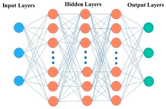
Figure 1.
Schematic diagram of the network structure for the model.
Table 5.
Model parameter information.
The elements in the propagate forward through the network, accomplishing a series of weighted summations and non-linear activations by the weight coefficient matrix w, bias vector b, and activation function. The computation is performed layer by layer from the input, hidden, and output layers until the result is output. The definition for the main parameters is as follows: network layer L, weight matrix w, bias vector b, activation function , the input , and output consist of m training samples: . The number of neurons in the input layer is defined as , and that in the hidden layer is defined as . The linear coefficients w and the bias vector b in the layer respectively constitute the weight matrix and the one-dimensional vector . The inactivated linear output z in the layer is composed of , and the output α of each layer consists of . First, the weight matrix w and the bias matrix b are initialized randomly, and the inputs of the model are set to so that the network is then calculated according to the following equation:
The activation function (ReLU) is defined as follows:
In view of the above, a series of hidden layers can be described as:
and the output layers are presented by the set of equations below:
In the Formulas (4) and (5), the superscripts represent the number of layers, and the subscripts correspond to the number of bits. The backpropagation obeys the chain rule of derivation, which is defined as follows:
In the Formula (6), y and z are the functions that map from real number to real number. The gradient of the mse (mean square error) loss function is determined from the backpropagation of the error e, and the mse is defined as follows:
where is the output and y is the actual value of the training sample, respectively. The training data in the model were divided into batches. The gradient descent and optimization were performed through the Nadam method to obtain the best weight and bias. The model randomly used neurons in the hidden layer to update for weight and bias values during the training. After the iteration ended, the model was reverted to its original form, and the loss function was minimized. The Nadam [28] method is an extension of the adaptive motion estimation (Adam) optimization algorithm, which uses Nesterov accelerated gradient (NAG) instead of vanilla momentum, combining Adam and NAG algorithms with an attenuation step () and a first-order moment hyperparameter to improve performance.
In this respect, the output layer gradient is as follows:
In the Formula (8), denotes the Hadamard product (the multiplication of the corresponding elements of the two matrices A and B of the same dimension). The common part of Equation (8) is denoted as :
The hidden layer gradient can be derived using mathematical induction as follows:
The corresponding gradients of and can be found as follows:
An update of the weights w and bias b for each layer with a batch size of 3 can be calculated as follows:
If all w and b values are less than the stop iteration threshold , the iteration should be stopped to display the linear relationship coefficient matrix and bias vector for each hidden and output layer.
3. Results
3.1. BP Neural Network Model Accuracy
Figure 2 displays the accuracy and loss function curves of the model. It can be seen in Figure 2a that the accuracy curve rises rapidly and remains above 0.92 after training for more than 1000 steps. It is worth mentioning that the model converges quickly due to the small data sample. According to Figure 2b, the loss curve of the model decreases rapidly within 1000 steps. Meanwhile, the value of the loss function gradually decreases to 0.00043 within 1001 to 8000 steps. These results indicate that the loss function is continuously decreasing toward the gradient, which represents the improvement in model accuracy. As seen in Figure 3, the linear regression coefficient (K) for the model prediction data and experimental data is 1.0331. In addition, the determination coefficient is 0.8944. The closer the value of is to 1, the better the goodness of fit and the higher the accuracy of the model. This means that the BPNN is suitable for predicting the mechanical properties of the joint.
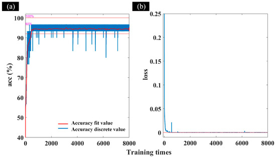
Figure 2.
Accuracy and loss function curves. (a) Accuracy curve, (b) Loss function curve.

Figure 3.
(a) Linear regression analysis of the predicted data and experimental data, (b) the corresponding residuals of characteristic data point.
3.2. Mechanical Properties Prediction and Process Optimization
The potential relationship between the process parameters and the mechanical properties of the joints can be expressed as follows:
In the Formula (13), the parameters referred to as T, Y, and E are the yield strength, tensile strength, and elongation of the joints, respectively; R is the rotational speed, V is the welding speed, and N is the welding pressure. In order to evaluate the effectiveness of the model, the theoretically predicted and experimentally obtained results were compared. As shown in Figure 4a,d,g, the curve as a whole first exhibits an upward trend and then decreases. Once the rotational speed increases from 1000 rpm to 1800 rpm, the mechanical properties of the joints increase and reach the peak at about 1800 rpm. At this time, the yield strength and tensile strength both exceed 400 MPa. With the continuous increase of the rotational speed, the three curves show a varying degree of decline. When the rotational speed and welding pressure are constant, through research on the influence of welding speed on joint mechanical properties, it is found that as the welding speed varies, the overall mechanical properties of joints show a downward trend (Figure 4b,e,h). Before the welding speed reached 200 mm/min, the curve slightly varied. As soon as the welding speed exceeded 200 mm/min, the curve rapidly declined. At the constant welding speed and rotational speed, the effect of the welding pressure on the joint mechanical properties was similar to that of the rotational speed (see Figure 4c,f,i). To sum up, the prediction curves passed through the sample data points in a smooth trend, further showing the good high-dimensional fitting “capacity” of the BPNN.
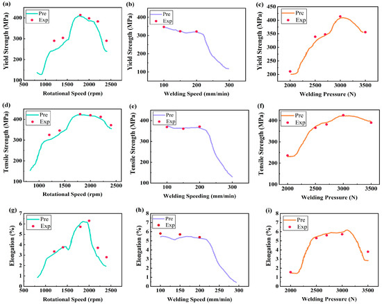
Figure 4.
Variation and fitting of Yield strength, Tensile strength, and Elongation with the Rotational Speed, Welding Speed, and Welding Pressure in measured and predicted data. (a,d,g): Welding Speed 100 mm/min and Welding Pressure 3000 N. (b,e,h): Rotational Speed 1600 rpm and Welding Pressure 3500 N. (c,f,i): Rotational Speed 1800 rpm and Welding Speed 100 mm/min.
Figure 5 depicts the 2195 aluminum alloy process window predicted by the model based on sample data. The maximum predicted tensile strength was 415 MPa, and the pink curved surface was used to represent all process parameters corresponding to the maximum predicted tensile strength (shown by the red arrows in Figure 5). The process parameters corresponding to the pink surface included the rotational speed between 1650 rpm and 1850 rpm, the welding speed between 100 mm/min and 110 mm/min, and the welding pressure between 2.9 kN and 3 kN. These process parameters were extracted from the above parameter ranges for experimental verification (Table 6). According to the results, the most optimal process parameter obtained from the validation tests were the values of 1810 rpm, 105 mm/min, and 3 kN for the rotational speed, welding speed, and welding pressure, respectively, at which the tensile strength of the joint reached 431 MPa, 82% of that of the base material. The difference between the predicted and experimental values was 3.71% (Figure 6). It is worth noting that the optimal tensile strength of the joint, established via machine learning, was higher than that from any set of previously collected data (Table 3). This indicates that the method used in this study has a significant advantage in process optimization.
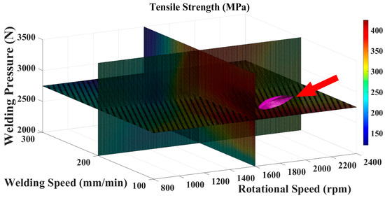
Figure 5.
The best set of process parameters surface.
Table 6.
Comparison of experiment and predicted results.
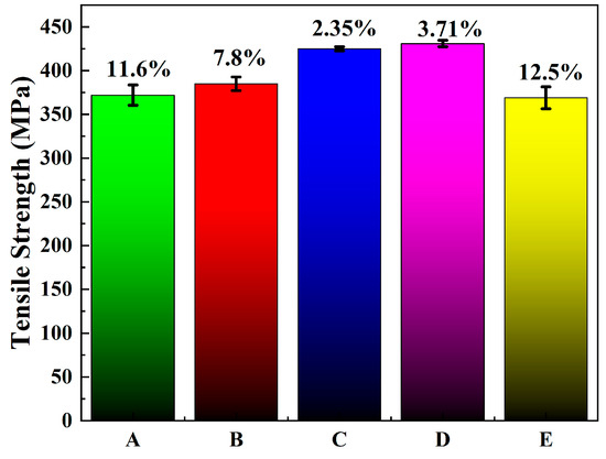
Figure 6.
The errors of optimal process parameters and experimental results.
4. Discussion
4.1. Relevance Analysis of Weld Forming and Joint Mechanical Property Prediction Results
Given the limitation of the “black box” characteristic of the BPNN, it is difficult to explain the changes in curves through a single data analysis. Therefore, in this study, the implied metallurgical mechanisms of the predicted mechanical properties of joints have been revealed by analyzing the joints forming characteristics. As shown in Figure 7, when the welding speed and welding pressure are constant, the low rotational speed can cause the emergence of a hole defect in a section of the joint (highlighted with a red square in Figure 7a). This is due to the fact that insufficient heat input at low rotational speed may result in poor material fluidity. The phenomenon explains why the above predictive curves demonstrated the decrease in the mechanical properties of the joints at lower rotational speeds (see Figure 4a,d,g). A further increase in the rotational speed leads to an increase in the heat input and the fluidity of the material, making the defects disappear (Figure b,c). Therefore, the mechanical properties of the joints have been improved. However, the heat input caused by the increase in rotational speed to 2500 rpm resulted in serious softening of the material, and the mechanical properties of the joint were rapidly reduced (Figure 4a,d,g). Similarly, when the rotational speed and welding pressure are constant, the hole defects can form at a welding speed of more than 250 mm/min (see the area highlighted with a red square in Figure 7f). This is owing to excessive welding speed, which yields insufficient welding heat input and material flow performance. Thus, the predicted curves of mechanical properties (Figure 4b,c,h) rapidly declined after the welding speed exceeded 200 mm/min. At a constant rotational speed and welding speed, the too-low welding pressure can induce the emergence of surface groove defects in the joint (see the red square in Figure 7g). The defects vanish with an increase in the welding pressure (Figure 7h,i). At this time, the yield strength, tensile strength, and elongation all show an increasing trend in varying degrees, with the increasing trend of yield strength being the most obvious (Figure 4c,f,i).
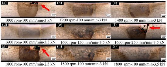
Figure 7.
(a–i): Macroscopic morphologies of cross-sections of FSW joints with different parameters (Red arrow points to the defects).
4.2. Influence of Process Parameter Changes on Mechanical Properties
Yield strength, tensile strength, and elongation are the three most important mechanical properties of the FSW joint. In this study, the welding data obtained from a machine learning model were analyzed to reveal the influence of welding process parameters on the mechanical properties of FSW joints, thereby guiding the joining process. Figure 8 depicts a four-dimensional slice diagram of the mechanical properties of the joints at different process parameters. The x-, y-, and z-axes in the diagram represent the welding pressure, welding speed, and rotational speed, respectively. The gradient changes in color represent the magnitudes of the yield strength, tensile strength, and elongation. The red-highlighted area, defined for simplicity as the process window, denotes the most optimal process parameter range. Figure 8a,d,g depict the slices of the mechanical properties of the FSW joint at different welding speeds. It can be found from Figure 8a that with the decrease in welding speed, the process window continues to increase, and the maximum process window corresponding to yield strength was achieved at a welding speed of 100 mm/min. Meanwhile, the process window is triangle-shaped, two sides of which are equal to 3500 N and 1500 rpm, respectively. This indicates that the closer the welding pressure to 3500 N for a fixed welding speed, the wider the range of the optional tool speed. Similarly, the range of the optional welding pressure becomes wider as the rotational speed approaches 1500 rpm. In other words, when the welding speed is constant, the rotational speed and welding pressure have a certain correlation with the yield strength. These results play a decisive role in the welding process. For example, if the pressing ability of the welding robot equipment is insufficient, the welding speed and rotational speed can be set close to 100 mm/min and 1500 rpm, respectively. In this case, the higher joint yield strength can be obtained at a welding pressure of 2500 N. When the welding speed is constant, the changes in the elongation with the rotational speed and welding pressure are similar to that in the yield strength (Figure 8g). However, for the tensile strength, the process window in the slice diagram at different welding speeds exhibits a rectangular shape (Figure 8d). This means that when the welding speed is constant, the impacts of welding pressure and rotational speed on the joints are independent of each other. Figure 8b,e,h display the sliced diagrams of the mechanical properties of FSW joints at different welding pressures. The maximum process window for the yield strength can be obtained at a welding pressure of 3500 N, and the process window itself is dumbbell-shaped (Figure 8b). The optional welding speed range is relatively large when the rotational speed is close to 1500 rpm. Therefore, it can be concluded that when a higher welding efficiency is required, the rotational speed should be close to 1500 rpm. In this case, the higher welding speed can be applied to achieve the satisfactory yield strength of the joint. For the tensile strength and elongation of the joint, the changing patterns of them with rotational speed and welding speed are similar to the yield strength (Figure 8e,h). Figure 8c,g,i depict the mechanical properties of the joints at different welding speeds. For the yield strength, the maximum process window can be obtained at a rotational speed of 1500 rpm. In this case, the process window possesses an approximately triangular shape (Figure 8c). This indicates that when the rotational speed is constant, the influence of welding speed and welding pressure on the yield strength is correlative. In turn, the variations in the tensile strength and elongation of the joint with the welding pressure and welding speed will be similar to that of the yield strength at the fixed welding speed, showing a triangular trend.
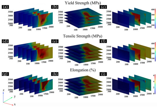
Figure 8.
Influence of welding parameters on mechanical properties of welding joints: (a–c) Yield strength, (d–f) Tensile strength, (g–i) Elongation.
Based on the above analysis, the welding speed and welding pressure can be set closer to 100 mm/min and 3500 N, respectively, when the rotational speed of the chief axis of the welding robot equipment is limited. At this time, the higher yield strengths of the joints can be obtained at lower rotational speeds. Similar assumptions are valid for tensile strength and elongation.
5. Conclusions
The BPNN model was established to predict the mechanical properties of the friction stir welded robot 2195 aluminum alloy joints so as to optimize their welding process. Based on the findings, the main conclusions can be drawn as follows:
- The accuracy of the BPNN could reach 92%, and the determination coefficient was 0.8944. The optimal process parameters for achieving high tensile strength of the joints were 1810 rpm, 105 mm/min, and 3000 N for the rotational speed, welding speed, and welding pressure, respectively. At these values, the predicted tensile strength was 415 MPa, only 3.71% lower than the experimentally obtained result (431 MPa). This indicates that the model fits the experimental data well.
- The prediction rationality of the model was verified via the microstructural analysis of the joints, and the latent metallurgical mechanism of the model was revealed. The prediction of the model was based on the change in heat input and material flow behavior caused by different welding parameters, which affected the mechanical properties of joints.
- The process window and the influence of process parameters on the mechanical properties were obtained. At a constant welding speed, the effects of rotational speed and welding pressure on the yield strength exhibited a certain correlation, and the process window corresponding to the higher yield strength and elongation was approximately triangular. In turn, the process window for the higher tensile strength was rectangular so that the two influences were independent of each other. At a constant welding pressure, the process window associated with elevated mechanical properties was approximately dumbbell-shaped. Finally, at a fixed rotational speed, the process window combining the high mechanical properties had a triangular-like shape.
Supplementary Materials
The following are available online at https://www.mdpi.com/article/10.3390/met13020267/s1, Figure S1: The image of the fractured specimen, Figure S2: Stress-strain curve.
Author Contributions
Conceptualization and methodology, Y.Z.; writing—original draft preparation, F.Y.; visualization, F.Y.; Experiment execution, Z.L.; formal analysis, Y.M.; supervision, Y.X.; project administration, F.Z.; funding acquisition, Y.Z.; writing—review and editing, F.Z.; All authors have read and agreed to the published version of the manuscript.
Funding
This research was funded by [the Guangdong Provincial Science and Technology Plan Project] grant number [2022A0505050054], [the National Natural Science Foundation of China] grant number [51905112], [the Young S&T Talent Training Program of Guangdong Provincial Association for S&T (GDSTA), China] grant number [SKXRC202221], [the Research and Development Program in Key areas of Dongguan] grant number [20201200300122] and [the National Key Research and Development Program of China] grant number [2020YFE0205300].
Institutional Review Board Statement
Not applicable.
Informed Consent Statement
Not applicable.
Data Availability Statement
Not applicable.
Conflicts of Interest
The authors declare no conflict interest.
References
- Mishra, R.S.; Ma, Z.Y. Friction stir welding and processing. Mater. Sci. Eng. R Rep. 2005, 50, 1–78. [Google Scholar] [CrossRef]
- Mendes, N.; Neto, P.; Loureiro, A.; Moreira, A.P. Machines and control systems for friction stir welding: A review. Mater. Des. 2016, 90, 256–265. [Google Scholar] [CrossRef]
- Saravanakumar, R.; Rajasekaran, T.; Pandey, C.; Menaka, M. Influence of Tool Probe Profiles on the Microstructure and Mechanical Properties of Underwater Friction Stir Welded AA5083 Material. J. Mater. Eng. Perform. 2022, 31, 8433–8450. [Google Scholar] [CrossRef]
- Du, Y.; Mukherjee, T.; DebRoy, T. Conditions for void formation in friction stir welding from machine learning. npj Comput. Mater. 2019, 5, 68. [Google Scholar] [CrossRef]
- Khalafe, W.H.; Sheng, E.L.; Bin Isa, M.R.; Omran, A.B.; Shamsudin, S.B. The Effect of Friction Stir Welding Parameters on the Weldability of Aluminum Alloys with Similar and Dissimilar Metals: Review. Metals 2022, 12, 2099. [Google Scholar] [CrossRef]
- Saravanakumar, R.; Rajasekaran, T.; Pandey, C.; Menaka, M. Mechanical and Microstructural Characteristics of Underwater Friction Stir Welded AA5083 Armor-Grade Aluminum Alloy Joints. J. Mater. Eng. Perform. 2022, 31, 8459–8472. [Google Scholar] [CrossRef]
- Meng, X.; Huang, Y.; Cao, J.; Shen, J.; dos Santos, J.F. Recent progress on control strategies for inherent issues in friction stir welding. Prog. Mater. Sci. 2020, 115, 100706. [Google Scholar] [CrossRef]
- Huang, Y.; Meng, X.; Xie, Y.; Wan, L.; Lv, Z.; Cao, J.; Feng, J. Friction stir welding/processing of polymers and polymer matrix composites. Compos. Part A Appl. Sci. Manuf. 2018, 105, 235–257. [Google Scholar] [CrossRef]
- Peng, C.; Jing, C.; Siyi, Q.; Siqi, Z.; Shoubo, S.; Ting, J.; Zhiqing, Z.; Zhihong, J.; Qing, L. Friction stir welding joints of 2195-T8 Al–Li alloys: Correlation of temperature evolution, microstructure and mechanical properties. Mater. Sci. Eng. A 2021, 823, 141501. [Google Scholar] [CrossRef]
- Xue, F.; He, D.; Zhou, H. Effect of Ultrasonic Vibration in Friction Stir Welding of 2219 Aluminum Alloy: An Effective Model for Predicting Weld Strength. Metals 2022, 12, 1101. [Google Scholar] [CrossRef]
- Dewan, M.W.; Huggett, D.J.; Liao, T.W.; Wahab, M.A.; Okeil, A.M. Prediction of tensile strength of friction stir weld joints with adaptive neuro-fuzzy inference system (ANFIS) and neural network. Mater. Des. 2016, 92, 288–299. [Google Scholar] [CrossRef]
- Yin, L.; Wang, J.; Hu, H.; Han, S.; Zhang, Y. Prediction of weld formation in 5083 aluminum alloy by twin-wire CMT welding based on deep learning. Weld. World 2019, 63, 947–955. [Google Scholar] [CrossRef]
- Agelet De Saracibar, C. Challenges to Be Tackled in the Computational Modeling and Numerical Simulation of FSW Processes. Metals 2019, 9, 573. [Google Scholar] [CrossRef]
- Karna, S.K.; Sahai, R. An Overview on Taguchi Method. Int. J. Eng. Math. Sci. 2012, 1, 11–18. [Google Scholar]
- Hill, W.J.; Hunter, W.G. A Review of Response Surface Methodology: A Literature Survey. Technometrics 1966, 8, 571–590. [Google Scholar] [CrossRef]
- Larson, M.G. Analysis of Variance. Circulation 2008, 117, 115–121. [Google Scholar] [CrossRef]
- Yuvaraj, K.P.; Ashoka Varthanan, P.; Haribabu, L.; Madhubalan, R.; Boopathiraja, K. Optimization of FSW tool parameters for joining dissimilar AA7075-T651 and AA6061 aluminium alloys using Taguchi Technique. Mater. Today Proc. 2020, 45, 919–925. [Google Scholar] [CrossRef]
- Singh, L.; Al Haque, M.S.; Singh, A.; Pun, A.K. Study and optimize tensile strength of FSW joints using AA5083 filler by Taguchi & Anova. Mater. Today Proc. 2022, 48, 1718–1722. [Google Scholar] [CrossRef]
- Saravanakumar, R.; Rajasekaran, T.; Pandey, C. Optimisation of underwater friction stir welding parameters of aluminum alloy AA5083 using RSM and GRA. Proc. Inst. Mech. Eng. E J. Process Mech. Eng. 2022, 095440892211344. [Google Scholar] [CrossRef]
- Baş, D.; Boyacı, I.H. Modeling and optimization I: Usability of response surface methodology. J. Food Eng. 2007, 78, 836–845. [Google Scholar] [CrossRef]
- You, J.; Zhao, Y.; Dong, C.; Wang, C.; Miao, S.; Yi, Y.; Su, Y. Microstructure characteristics and mechanical properties of stationary shoulder friction stir welded 2219-T6 aluminium alloy at high rotation speeds. Int. J. Adv. Manuf. Technol. 2019, 108, 987–996. [Google Scholar] [CrossRef]
- Effertz, P.S.; de Carvalho, W.S.; Guimarães, R.P.M.; Saria, G.; Amancio-Filho, S.T. Optimization of Refill Friction Stir Spot Welded AA2024-T3 Using Machine Learning. Front. Mater. 2022, 9, 864187. [Google Scholar] [CrossRef]
- Manvatkar, V.D.; Arora, A.; De, A.; DebRoy, T. Neural network models of peak temperature, torque, traverse force, bending stress and maximum shear stress during friction stir welding. Sci. Technol. Weld. Join. 2012, 17, 460–466. [Google Scholar] [CrossRef]
- Lakshminarayanan, A.K.; Balasubramanian, V. Comparison of RSM with ANN in predicting tensile strength of friction stir welded AA7039 aluminium alloy joints. Trans. Nonferrous Met. Soc. China 2009, 19, 9–18. [Google Scholar] [CrossRef]
- Jayaraman, M.; Sivasubramanian, R.; Balasubramanian, V.; Lakshminarayanan, A.K. Application of RSM and ANN to predict the tensile strength of Friction Stir Welded A319 cast aluminium alloy. Int. J. Manuf. Res. 2009, 4, 306–323. [Google Scholar] [CrossRef]
- Rathinasuriyan, C.; Sankar, R.; Shanbhag, A.G.; SenthilKumar, V.S. Prediction of the Average Grain Size in Submerged Friction Stir Welds of AA 6061-T6. Mater. Today Proc. 2019, 16, 907–917. [Google Scholar] [CrossRef]
- Ba, J.L.; Kiros, J.R.; Hinton, G.E. Layer Normalization. arXiv 2016. [Google Scholar] [CrossRef]
- Ruder, S. An Overview of Gradient Descent Optimization Algorithms. arXiv 2017. [Google Scholar] [CrossRef]


Disclaimer/Publisher’s Note: The statements, opinions and data contained in all publications are solely those of the individual author(s) and contributor(s) and not of MDPI and/or the editor(s). MDPI and/or the editor(s) disclaim responsibility for any injury to people or property resulting from any ideas, methods, instructions or products referred to in the content. |
© 2023 by the authors. Licensee MDPI, Basel, Switzerland. This article is an open access article distributed under the terms and conditions of the Creative Commons Attribution (CC BY) license (https://creativecommons.org/licenses/by/4.0/).