Abstract
Single Al wires from unused AAAC (A50) cables were studied after laboratory fatigue testing, which simulated processes arising in these wires during their operation in the cables of overhead power lines (OPLs) and are valuable for predicting the lifespan of cables of OPLs. These wires, which were either fractured during testing (maximum loads—149.4–155.9 MPa; number of cycles till rupture—83,656–280,863) or remained intact, were examined by X-ray diffraction, electron backscatter diffraction, densitometry, and acoustic methods. An analysis of the structural, microstructural, and elastic-microplastic properties of the wires revealed common characteristics inherent in the samples after operation in OPLs and after fatigue tests, namely a decrease in the integral and near-surface layer (NSL) densities of the wires, a decrease in their Young’s modulus and microplastic stress, and an increase in the decrement. However, the tests did not fully reproduce the environmental influence, since in contrast to the natural conditions, no aluminum-oxide crystallites were formed in NSLs in tests and the microstructure was different. A comparison of the characteristics of the broken and unbroken wires allows us to suggest that the fastening locations of the wires are crucial for their possible failure.
1. Introduction
Predicting the duration of operation of Al wires of overhead power lines (OPLs) is one of the most important issues from a practical point of view. To understand the peculiarities of destruction, laboratory studies are required that imitate the processes occurring de facto during the operation of OPLs. It is known that wires in real conditions are subjected to various types of mechanical loads, such as tension, vibration, and friction during vibration. Most high-voltage power lines are operated with relatively low tension, about 20% of the nominal strength value [1], which should ensure their long-term operation in accordance with regulatory documents. Nevertheless, a wide range of studies are aimed precisely at establishing the causes of the premature destruction of wires and the possibility of predicting their “lifetime”. For these purposes, numerous and diverse experimental mechanical fatigue (for example, [2,3,4,5,6,7,8,9,10,11,12,13,14,15]) and wear ([16,17]) tests were carried out and theoretical modeling of crack trajectories and wire endurance during the fatigue tests was performed (for example, [6,10,12,18,19]), taking into account various factors simulating the impact on the wire in real OPLs leading to a wire fracture (average pre-load tensile stress [2,3,4,10,19], amplitude of the bend and the type of conductor-clamp connection [5,6,7,8,9,12], presence of steel core [9], the chemical composition of the aluminum wires in the cables [8], geometric discontinuities of the wires [18]).
For fatigue tests and theoretical modeling, both entire aluminum cables (conductors) [2,3,4,5,6,7,8,9,11,14,16,17] of the All Aluminum Alloy Conductor (AAAC) [6,7,8,9,16,20] and Aluminum Conductor Steel Reinforced (ACSR) [2,11,13,14,16,17,19] types of different modifications, used in the real OPLs and prepared from the Al of different grade of purity, were taken, as well as single aluminum wires from the AAAC [15,18] and ACSR [13] conductors or two single aluminum wires crossed at an angle of 29–30° from the ACSR cables [10,12]. Finite element analysis and other related methods [6,10,12,18,20], in addition to a study utilizing artificial neural networks [19] and several analytical approaches [2,3,6,10,20], were concurrently used to model the fatigue process in the wires and its results and to predict the lifetime of the wires during fatigue tests.
One of the main tasks of fatigue testing is obtaining of the Wöhler curve, which is constructed after conducting fatigue tests on a large number of samples with different maximum values σmax of the alternating (cyclic) load applied to the sample during the tests (see examples in [2,3,4,5,6,7,8,9,10,12,13,14,15,18]). The Wöhler curve is also often referred to as the S–N curve, where S is the maximum load σmax applied to the sample during cyclic fatigue tests, and N is the number of load cycles before the sample (wire or entire cable) fractures. The construction of the S–N curve allows us to estimate the value of the conditional endurance limit Se of the sample, above which the value σmax should not rise, as well as to estimate the number of cycles N during fatigue tests before the destruction of the sample at a given value of the maximum cyclic load σmax. In other words, the construction of the Wöhler curve fulfils the main task of fatigue testing to predict the “service life” of the sample during fatigue tests. However, it should be noted here that the strain of individual wires in the ACSR cable was measured during fatigue tests conducted in [11], and it was concluded that the alternating (cyclic) stresses, which are equal to traction loading, are not ideal fatigue indicators due to weak correlation with the experimental results.
So, part of the research is aimed at obtaining an experimental dependence of the number of cycles and stress to build calculation models in order to predict fatigue life [2,3,6,10,18]. Other studies present optical [2,5,6,7,10,12,16] and scanning electron [4,5,9,12,16,17] microscopy (OM and SEM) images for crack growth analysis [4,5,9,12] and fractographic analysis of the fracture surface of wires [2,4,5,7,9,10,12]. It should be noted that these OM and SEM and fractography data are mainly the qualitative data concerning the classification of the fracture surface type and mode of fracture. For example, for aluminum wires from cables types such as AAAC [4,7,9] and ACSR [2,5,10,12] of various modifications, three types of fracture surfaces are observed, having the form of a chip at 45° [2,4,5,7,9,10], V-like type [2,4,5] and quasi-smooth (quasi-planar [2] or quasi-normal [9]) [2,5,7,9]. The dominant part of the fracture surface is dependent on the type of cables, the location of the wire in the cable during fatigue testing (for the entire cables under the tests), and loading history of the samples. Two distinct zones were detected in [5] for Al wires from the ACSR cable after fatigue tests, showing a flat and fibrous microstructure with faint striation marks in the flat fracture surface.
In addition, Al wires from cables of AAAC [4] and ACSR [5] types after fatigue tests were studied by energy dispersive X-ray spectroscopy (EDS), which showed increased oxygen content in the areas with traces of fretting, with the possible formation of Al2O3 [4] and SiO2 [4,5] particles at the micro-slip zones.
Thus, the investigation of the properties of the Al wires after fatigue tests (and Al wires from cables after fatigue tests) was limited only by qualitative methods of studying their microstructure by OM and SEM methods and their chemical composition by the EDS method. Studies of the structure and elastic-microplastic properties of the wires after the fatigue tests have not been conducted.
Previously [21,22,23], we have studied changes in the structure, microstructure, and elastic-microplastic properties of individual Al wires from AAAC (A50) and ACSR (AC50/8) cables of different service lifespans, from 0 to 20 years (for AC50/8) and to 62 years (A50), in OPLs in the Volgograd region of Russia (designations A50 and AC50/8 are according to the Interstate Technical Standard GOST 839-2019 [1]; the AC50/8 cable, shortened hereafter to AC50, is similar to A50 but with a steel core instead of the central Al wire and with a larger nominal diameter of the component wires, 3.2 mm, in comparison to 3.0 mm for the A50 cable). Those studies were carried out using X-ray diffraction (XRD), electron backscatter diffraction (EBSD), densitometry, and the acoustic method of a composite resonator.
Similar to the Al wires from the cables after exploitation in the OPLs in natural environmental conditions, it is expected that the Al wires after laboratory fatigue tests will be characterized by modified structural, microstructural, and elastic-microplastic properties.
To prove this assumption, to make up for the lack of quantitative information about modifications in the structural, microstructural, and elastic-microplastic properties of Al wires after fatigue testing, and to compare the natural changes found in Al wires of OPL cables under environmental operating conditions, with the changes observed in wires after laboratory fatigue tests, in the current work, the same methods (XRD, EBSD, densitometry, and acoustic method) are applied to wires from unused AAAC A50 cables after laboratory tests [15] in fatigue mode. The loading frequency in [15] was chosen to be about 3 Hz. It is this kind of vibration that leads to the greatest cable fatigue [2] when added to the static tension of a cable. Only the impact in the mode of fatigue loading causes further cable fracturing.
In addition to the structural, microstructural, and acoustic characterization of the wires after the low-frequency fatigue testing, this study also attempts to determine the area of the premature cable fraction based on the analysis of changes in the structural, microstructural, and elastic-microplastic characteristics of aluminum wire samples (depending on the location along the length of a tested sample).
2. Materials and Methods
2.1. Samples
According to [1], an AAAC stranded cable, referred to as A50, consists of six Al wires with a nominal diameter of 3.00 mm, which are wound around a central Al wire of the same diameter, giving the wire a cross-sectional area of 49.5 mm2 ≈ 50 mm2 (hence the designation “A50”). Confirmation with an optical microscope showed that the actual diameter of the wires studied was 2.97–3.00 mm; see Table S1 in Supplementary Materials.
For the convenience of further use of the data and due to the importance of a detailed description of the history of the samples used for the current study, let us first briefly describe the fatigue tests of these samples conducted in [15]. To perform fatigue test in the cyclic tensile-relaxation mode [15], the outer Al wires were taken from a strand of a new A50 cable (sample N5-2 in [21,22,23]). Eleven samples were taken from one wire for fatigue testing. Specimens were made in the form of wire pieces with a total length of 200 mm and a working-part length of 100 mm. As in the case of actually operated wires, no special surface preparation was carried out before the fatigue test. Optical microscopy (OM) photographs of unused wires (Figure S1 in the Supplementary Materials as an example) demonstrate that the surface of the samples is not perfectly smooth. All the wires have surface defects, as well as those that were actually used for cables in OPLs. Obviously, this is due to both the manufacturing process of individual wires and cables and transportation. Nevertheless, the spread of experimental points on the obtained Wöhler curve was insignificant (see the results of fatigue tests given in [15]). To study the structural, microstructural, and elastic-microplastic properties, three samples were selected from these eleven specimens, which underwent cyclic tensile fatigue tests at room temperature under various maximum loads σmax. Two of these wires were brought to destruction during testing (i.e., these wires were used for the construction of the Wöhler curve in [15]) and one did not break. In addition, for comparison, one wire was examined in its original condition before fatigue tests.
In the fatigue tests, wire was rigidly fixed in the clamps and mounted on the testing machine Instron 8850 250 kN (Instron, Norwood, MA, USA) in the grips (holders) in such a way that the grip installed in the bottom part of the testing machine (Figure S2 of Supplementary Materials) was firmly fixed and did not move, while the grip in the upper part of the machine was able to move vertically. A variable load was applied to the wire through a clamp fixed in a movable grip. Hereafter, the upper grip with the ability to move (together with the wire clamp) is referred to as “movable” or “non-fixed” and, accordingly, the bottom grip (clamping the other end of the wire) is referred to as “immovable” or “fixed”.
The change in the tensile load on the sample according to the “Loading-Relaxation” scheme was carried out according to a sinusoidal law with a frequency of 3 Hz and the asymmetry coefficient R = 0.1 at maximum loads σmax close to the conditional endurance limit of Se = 158 ± 4 MPa, determined in [15] for one of the Al wires of the A50 cable, N5-2. Test conditions (number of cycles N, maximum load σmax, maximum force Fmax, and cycle load range Δσ) are given in Table 1, as well as the visual results of the fatigue tests: destruction (rupture) of two samples marked as C7 and C8 and no visible damage of the sample C10. The C7 and C8 wires broke in areas near one of the clamps (the one that was fixed in the movable grip), which is shown as an example in the Supplementary Materials Figure S2c, and schematically in Figure 1, where this clamp is indicated by the number 1, and the clamp in the fixed grip, respectively, by the number 2.

Table 1.
Cyclic fatigue test conditions for Al wires of A50 cables.
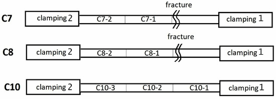
Figure 1.
A diagram of the wires (Table 1) from which samples were cut out for XRD and acoustic measurements (Supplementary Materials Table S1) after cyclic tests.
Sample 5-2 in Table 1 represents the initial state of an Al wire before testing. Samples C7 and C8 were tested for fatigue at different maximum loads, σmax = 149.4 MPa and 150.7 MPa, respectively, and withstood a different number of cycles before failure. Sample C10 tested at σmax = 155.9 MPa was not led to failure and was chosen for studies as an intermediate state between the initial sample and those that failed during fatigue testing.
The parts marked in Figure 1 as C7-1 and C8-1 are the wire fragments that are as close as possible to the area of destruction (rupture) that occurred near the movable grip 1. Parts C7-2 and C8-2 are wire fragments more remote from the area of destruction and closer to the grips of the test facility, near which no destruction was observed. Sample C10 was not led to failure and the working part of the wire was divided into three parts, where C10-2 is the central fragment of the wire and C10-1 and C10-3 are the parts located closer to the grips of the test setup (C10-1 near the movable (non-fixed) grip 1 and C10-3 near the fixed (immovable) grip 2). A detailed layout of the different parts is shown in Figure 1.
To study the wires by the densitometry method, long pieces of wires with lengths of 61–80 mm were cut from the longer part of the working area of the destroyed samples (i.e., parts C7-1 and C7-2 in one uncut piece for sample C7 and parts C8-1 and C8-2 in one uncut piece for sample C8). For densitometric measurements of the uninjured sample C10, the entire working part 100 mm long was used cut from the wire after fatigue testing (parts C10-1, C10-2, and C10-3 in one piece together).
After measuring the integral density of the wires by densitometry, to study the elastic and microplastic properties by acoustic methods as well as for XRD measurements, samples of smaller length ~25 mm were cut off from these long samples; that is, from the areas indicated in Figure 1 as C7-1, C7-2, C8-1, C8-2, C10-1, C10-2 and C10-2. The exact lengths l and diameters d of the samples of Al wires studied by acoustic and XRD methods are given in Supplementary Materials Table S1. Facets of the cross sections of the samples were prepared to perform the EBSD studies.
2.2. Experimental Details of Measurements
The experimental details of all measurements by OM, densitometry, XRD, EXD, SEM, and EBSD methods, as well as by the acoustic-resonance method of a composite piezoelectric resonator, are described in detail in [21,22,23]. The main details of the measurements and analysis are briefly given in Supplementary Materials Section S2, including the names of the manufacturers of the devices on which the measurements were carried out. Here, only the main peculiarities related to the measurements are given very briefly.
Due to the design features of the desktop X-ray powder diffractometer (D2 Phaser (Bruker AXS, Karlsruhe, Germany)) used in the current study, the temperature in the sample chamber during XRD measurements was equal to 314 ± 1 K. All other measurements (OM, densitometry, EDX, SEM, EBSD, and acoustic) were carried out at the room temperature.
Since the XRD patterns were measured from the long side of the Al wire samples in the form of a cylinder with the length of ≈25 mm, the diffracted X-ray signal came mainly from the penetration depth limited by the X-ray absorption in the Al material of the wires. According to the estimates made in [21,22,23], as well as shown in Supplementary Materials Section S2, the maximum penetration depth achieved by Cu-Kα X-ray radiation corresponds to the Al reflection with the maximum observed Bragg angle of 2θB ≈ 137.3° (reflection of Al with Miller indices hkl = 224 registered in this study) and is Tpen ≈ 36 μm. Thus, the mean structural and microstructural parameters obtained in the current XRD investigations are averaged over all observed Al reflections and characterize the Al-wire near-surface layer (NSL) with a thickness of Tl ≈ 36 μm only. XRD gives for this NSL the values of the average parameter a of the cubic unit cell of the Al material and the mass density ρX calculated from this parameter (see Formula S4 in Supplementary Materials), as well as the average sizes D of coherent X-ray scattering areas (crystallites) and microstrains εs in them. All these characteristics are obtained from analysis of the XRD reflections diffracted from atomic planes parallel to the wire surface, i.e., they correspond to the characteristics of the Al material in the direction perpendicular to the wire surface but not in the longitudinal direction.
The EBSD maps were taken at the centers of the cross-sections of the wires and at ~150 μm from the outer surface of the wires. The first EBSD maps correspond, obviously, to the bulk of the wire, and the second ones give information about NSL at a depth of ~150 μm from the wire surface. The analysis of EBSD maps leads to different characteristics of grains in the wire material, i.e., particles that, as a rule, contain several crystallites. These characteristics include individual and average (Dgrain) grain size, grain misorientation angles φmis, relative areas Srel occupied by grains, and grain aspect ratios. It should be emphasized once again that all the parameters obtained in the current EBSD study are characteristics of the cross-section of the wires (but not the longitudinal one). In addition, in the SEM investigation of the wires ruptured during the fatigue tests, the SEM images were obtained from the edges at the ends of the broken wires. Therefore, EBSD and SEM are methods that investigate the sample surface. Nevertheless, with appropriate sample preparation (cross sections for EBSD or the end of the rupture site for SEM), these methods allow data to be obtained on both the bulk and NSL of the wire
Unlike XRD, SEM, or EBSD, densitometry and acoustic methods characterize the entire volume of the wire, including both the volume part and the NSL.
3. Results
3.1. Densitometry Results
The density of the parts of each wire after cyclic fatigue tests was determined by the hydrostatic (densitometry) method. The results are shown in Figure 2 and Supplementary Materials Table S1. It was found that, for samples C7 and C8 which were destroyed during fatigue testing, the density of parts C7-1 and C8-1 of these samples, those parts located near the fracture areas, is noticeably lower than the density of parts C7-2 and C8-2 far from them.
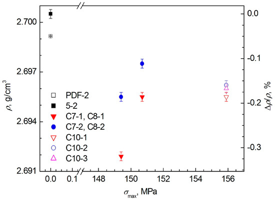
Figure 2.
Integral mass density ρ of samples according to densitometric measurements depending on the maximum load σmax of cyclic fatigue tests. The density defect Δρ/ρ was calculated taking the integral density of the initial sample 5-2 as ρ0 to calculate the difference Δρ = ρ − ρ0. The value indicated as PDF-2 in the Figure corresponds to the data by [24], Powder Diffraction File-2 (PDF-2) [25] card 01-071-4008 at a temperature T = 298 K close to the room temperature of densitometric measurements.
Compared to the initial state (sample 5-2), the value of the decrease in mass density Δρ/ρ for the samples C7-1 and C8-1 cut from the regions of wires near the fracture was −0.32(1)% and −0.19(1)%, respectively, and −0.19(1)% and −0.11(1)%, correspondingly, for samples C7-2 and C8-2 from the regions far from the fracture.
For the C10 sample, it was found that closer to the C10-1 and C10-3 clamps, only a slight decrease in density appeared relative to its central part C10-2 (Δρ/ρ = −0.19(1)%, −0.17(1)%, and −0.16(1)%, respectively). So, densitometric measurements of different parts of the C10 sample, which was not destroyed during fatigue tests, revealed a different decrease in the mass densities of the parts, although with the difference between them being within one or two estimated standard deviations (e.s.d.s) only.
3.2. XRD Results
Manifesting the polycrystalline nature of the wires, all studied aluminum wires before and after fatigue tests are characterized by similar radiographs, which contain all possible reflections of Al (space group , a = 4.04932(2) Å at 298 K [24] and a = 4.050694 Å at temperature T = 312.3 K [26], which is close to the temperature of XRD measurements, T = 314 K), as proved by X-ray phase analysis using the program EVA [27]. As an example, Figure 3 shows an XRD pattern of one of the samples. For the remaining samples, the XRD patterns are presented in Figure S3 of the Supplementary Materials.
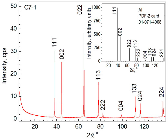
Figure 3.
XRD patterns from sample C7-1. Miller indices hkl of Al reflections are indicated. The inset shows the XRD pattern of the Al phase according to PDF-2 card 01-071-4008 [26] at a temperature T = 312.3 K, which is close to the temperature of XRD measurements, T = 314 ± 1 K.
Visual inspection of XRD patterns of various Al wire samples before and after the fatigue test (Figure 3 and Figure S3) indicates that the intensities of Al reflections are clearly influenced by the effects of preferential orientation along the crystallographic direction of Al [011]. The presence of this preferential [011] orientation is expressed in the XRD patterns from the samples by the increased intensity of reflection with the Miller indices hkl = 022 compared to the Al XRD pattern from the PDF-2 powder database (compare the inset in Figure 3 with the XRD patterns from the samples). Moreover, the analysis of changes in the maximum intensities Imax of Al reflections shows that with an increase in load value σ during cyclic fatigue tests and depending on the location of the sample in the tested wire (Figure 1), the effect of preferential orientation along [011] is systematically enhanced (see Figure 4, Table S2 and a more detailed discussion in Supplementary Materials Section S2).
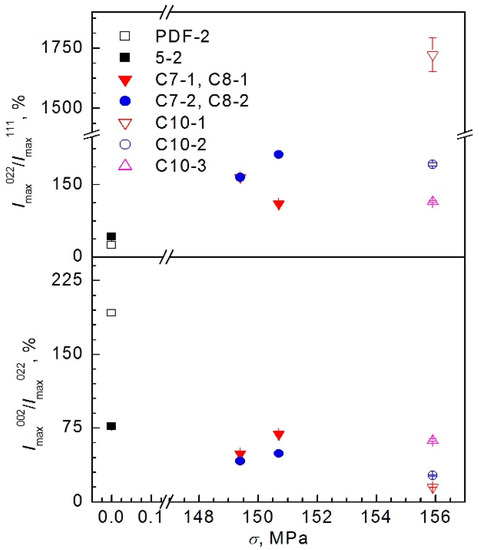
Figure 4.
Dependence of the ratio of the maximum intensities (a) Imax022/Imax111 of reflections 022 and 111 and (b) Imax002/Imax022 of reflections 002 and 022 on the load σ during cyclic loading of the samples. The designation “PDF-2” corresponds to the data of the powder database map PDF-2 01-071-4008 [26] at a temperature T = 312.3 K, which is close to the temperature of XRD measurements, T = 314 ± 1 K.
Previously [21,22,23], a similar enhancement of preferential orientation along the [011] direction has been also noted in Al wires of the cables of the A50 and AC50 types with a service life of up to 62 and 20 years, respectively. At the same time, for external Al wire from an ACSR type stranded cable that has operated in OPL for 40 years [28], the intensity of Al reflections did not show the effect of preferential orientation (according to the XRD pattern given in [28], the ratio of maximum reflection intensities Imax022/Imax111 and Imax002/Imax022 is ≈ 24% and ≈ 200%, which is close to the corresponding values 23.9% and 190.8% in Al powder [24], free from preferential orientation). Additionally, in contrast to OPL cables of AAAC and ACSR types, which were used under natural environmental conditions, where XRD studies showed the formation of weak reflections assigned to aluminum oxides (δ- and/or δ*-Al2O3) [21,22,23] or α-Al2O3 and α-SiO2 [26], no reflections of either aluminum oxides or other impurity phases were found after laboratory fatigue testing by cyclic loading of unused A50 wires. Probably, the observed difference in the preferential orientation of Al reflections and the difference in the impurity phases for wires in the current work and in [21,22,23] compared to [28] is due to the difference in the manufacture of wires and environmental conditions of their use (respectively, the Volgograd region of Russia and North Bohemia region of Czech Republic).
A comparison of reflections with the same Miller indices in the measured XRD patterns showed that the Bragg angles 2θB of reflections from samples after different stages of fatigue testing and from different locations in relation to the sites of grip and destruction differed only for wires with a different service life in power lines [21,23]. An illustration of the shift of reflections in XRD patterns along the diffraction angle 2θ is shown in Figure S4 of the Supplementary Materials using the Al reflection with Miller indices hkl = 133 as an example. This shift in the angular positions of the XRD reflections indicates a change in the parameter a of the cubic unit cell of Al wires after fatigue tests.
The parameters a of the cubic unit cell of the Al material of the wire samples after different stages of cyclic loading are shown in Figure 5a and in Supplementary Materials Table S2. They were calculated using the Celsiz [29] program, which applies the least-squares method and works with the observed Bragg angles 2θB after making the necessary angular corrections. Figure 5b shows mass densities ρX (hereinafter referred to as “XRD mass densities”, “XRD densities”, or “X-ray densities”) recalculated from volume Vcell = a3 and the mass of the unit cell of the crystalline aluminum; see the recalculation formula and conversion coefficient of atomic mass units to grams [30] in [21,22,23] and in Supplementary Materials Section S2. As noted in Section 2.2, the XRD densities ρX in the case of the Al wires and used Cu-Kα X-ray radiation are a characteristic of the wire NSL with a thickness of T ≈ 36 μm.

Figure 5.
(a) Average parameter a of the cubic unit cell and (b) average XRD mass density ρX of the Al material of the near-surface layer with a thickness of ≈36 μm of the samples after cyclic loading as a function of the applied maximum load σmax. The right ordinates show the values of (a) the defect Δa/a of the unit cell parameter and (b) the defect of the XRD density ΔρX/ρX, where Δa = a−a0 and ΔρX = ρX−ρX0, a0 and ρX0 are, respectively, the unit cell parameter and XRD density of unused sample 5-2 not subjected to cyclic loading. The designation “PDF-2” in (a,b) corresponds to the data of the powder database map PDF-2 01-071-4008 [26] at a temperature T = 312.3 K, which is close to the XRD-measurement temperature T = 314 ± 1 K.
In a new, unused sample 5-2, the parameter a0 of the unit cell (hereinafter, the index “0” means the value referring to the unused sample 5-2 not subjected to cyclic loading or operation in OPLs) is a bit smaller, and, accordingly, the X-ray density ρX0 is somewhat higher than that in Al powder, borrowed from the PDF-2 powder database (at approximately the same temperature of measurements as in the present experiment). The integral mass density ρ of the unused Al wire N5-2, measured by the densitometric method, is also somewhat higher than the density borrowed from PDF-2 (Table S2 of Supplementary Materials and Figure 2 and Figure 5b, density defects for Al from PDF-2 Δρ/ρ = −0.050(1)% and ΔρX/ρX = −0.033(7)% in the case of mass density measured with the densitometric method and calculated from XRD data, respectively, if density defects are assumed to be zero in the initial sample 5-2). As was previously noted [23], this difference could be explained by a small admixture of contaminating elements with a smaller Slater radius, such as Si, which are present in the wire material according to the passport nominal composition and EDX results.
Since ρX ~ 1/Vcell, the tendencies of change in both a and ρX with the change in the magnitude of the cyclic load are opposite, i.e., lattice stretching (an increase in the unit-cell volume Vcell) of Al material of the wires corresponds to a decrease in the density ρX of this material. Thus, it is sufficient to consider trends in only one quantity, either ρX or a.
The cyclic loading of previously unused A50 wires leads to a decrease in the XRD mass density ρX of Al-wire NSLs with a thickness of ≈36 μm. In addition, the drop in ρX is greater for wire samples C7-1 (ΔρX/ρX = −0.20(1)%) and C8-1 (ΔρX/ρX = −0.15(2)%), which were cut from sites near the grips (Figure 5b), where as a result of cyclic loading, the initially-long wires were destroyed. At the same time, samples C7-2 and C8-2 cut far from the capture region show a smaller decrease in density (ΔρX/ρX = −0.05(2)% and −0.08(1)%, respectively). So, with an increase in the maximum cyclic load from σmax = 149.7 MPa (samples C7-1 and C7-2) to σmax = 150.7 MPa (C8-1 and C8-2), the difference in densities between the samples cut at the grips (destruction region) and far from them declines.
This observation is in a good agreement with the results obtained for samples C10-1, C10-2, and C10-3 after cyclic loading with an even higher load σmax = 155.9 MPa, which, however, did not lead to failure. Analogously to the samples after cyclic loading with lower loads, a decrease in the density ρX is observed. However, the difference in the XRD densities of samples from the regions near captures (ΔρX/ρX = −0.057(21)% and −0.064(14)% in C10-1 and C10-3, respectively) and far from them (ΔρX/ρX = −0.053 (17)% in C10-2) is noticeably less than for samples C7-1 and C8-1 and matches that in C7-2 and C8-2 for both wires failed as a result of cyclic loading at lower loads. Moreover, as can be seen, although within the standard deviation (e.s.d.), in area far from the captures (C10-2), the same tendency is observed of a decrease in ρX, which is smaller than near the captures (C10-1 and C10-3), just as in wires, led to destruction.
Comparing the results of the measurements, it was found that the XRD values of the densities ρX of the wires are close to the integral densities measured by the densitometric method, ρ, but, as a rule, somewhat less (cf. Supplementary Materials Tables S1 and S2 and Figure 2 and Figure 5b). This observation can be obviously explained by the fact that, as mentioned above, the XRD mass density ρX is the average density of a NSL, with a thickness of ≈36 μm, while the integral mass density ρ measured by densitometry is the value averaged over the entire volume of the sample. In NSL during cyclic loading (as well as during use in natural conditions in OPLs), a greater number of defects of a void nature can form and a greater lattice stretch occurs due to defects compared to the bulk of the wire, which leads to a smaller density ρX in comparison to integral density ρ. The observed deviations for both ways are possible due to the individual characteristics of the wire samples and their cyclic loading (for example, due to the presence of defects in the initial sample).
Despite some difference in the values of ρ and ρX, the trends discussed above for the X-ray density ρX hold true for the density ρ measured by densitometry (cf. Figure 2 and Figure 5b). Changes in ρ with a change in load σmax during fatigue tests do not occur as smoothly as in the case of ρX, which can probably be explained by either experimental errors during measurements or the individual characteristics of the samples.
Upon comparing the Al reflection with Miller indices hkl = 111 in the insets to Supplementary Materials Figure S3a–g and the Al 133 reflection in Supplementary Materials Figure S4, one can see that the reflection profiles before and after different stages of cyclic loading are characterized by different FWHM. This difference indicates a change in the parameters of the microstructure of the wires because of their fatigue modification due to cyclic loading.
The average crystallite sizes D0 calculated in the model with zero microstrain (εs = 0) show a decrease from D0 ~ 110 nm in in the unused sample 5-2 and in samples C7-1 and C7-2 to ≈60–94 nm in samples C10-1, C10-2 and C10-3 when the maximum load σmax increases from 144.9 MPa up to 155.9 MPa (see Table S2 and Figure S5 in Supplementary Materials Section S3).
However, using the graphical analysis of XRD-reflection profiles, namely the Williamson–Hall plot (WHP) [31] and Size-Strain plot (SSP) [32], it has been found recently [21,23] that in wires from A50- and AC50-type cables of air power transmission lines, characterized initially by the absence of microstrains (εs = 0), microstrains are formed after use of the wires in natural conditions for a period of 8 years or more. Due to the presence of a stabilizing steel core, there are slightly less microstrains in AC50 wires (εs ≈ 0.025%) compared to A50 wires (εs ≈ 0.032%).
In order to verify the presence of local microstrains in Al wires from A50-type cables after cyclic-loading-fatigue testing, a profile analysis of the observed Al reflections was carried out for all the samples studied. The plotted WHP and SSP plots for all fatigue-test specimens from Table 1 are shown in Figures S6–S8 of Supplementary Materials (for the unused new specimen 5-2, WHP and SSP plots can be found in [21]). All calculations of microstructural parameters from the XRD reflection profiles by the WHP and SSP methods were performed using the SizeCr [33] program in accordance with the procedures for pV type reflections, which were observed in the XRD patterns of the samples (for the samples, the criterion determining the type of reflection showed the values FWHM/Bint = 0.74(3)–0.83(4), which are typical to pV reflections [34], where Bint = Iint/Imax is the integral width of a reflection with integral intensity Iint and maximum intensity Imax). The quantitative results of WHP and SSP on the obtained microstructure parameters (average crystallite size D and absolute value of the average microstrain εs) are summarized in Table S2 of the Supplementary Materials and graphically in Figure 6.
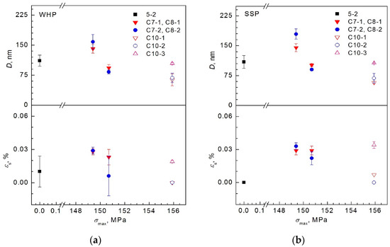
Figure 6.
Microstructure parameters (average sizes D of crystallites of Al material of wires and absolute average values of microstrains εs in them) for samples subjected to cyclic loading with different magnitudes of maximum load σmax, according to the results of calculations by methods of (a) WHP and (b) SSP.
A comparison of the results obtained by the WHP and SSP methods (Supplementary Materials Table S2 and Figure 6a,b) shows that both methods give close results confirming each other. Yet, the WHP technique is more illustrative, since the negative or zero slope of the approximating straight line in the case of a WHP of a sample with εs = 0 is immediately visible. In contrast to WHP, the approximating straight line of the SSP graph in the case of εs = 0 has a zero or negative intersection with the abscissa; however, with a very small absolute value, as a rule, that is difficult to detect visually. Nevertheless, in most cases, the SSP plots are characterized by a much smaller spread of points around the approximating straight line (see Figures S6–S8 of Supplementary Materials). As a result, in the case of SSP, the value of the determination coefficient Rcod [31,33], which characterizes this spread, is closer to 100%. For example, the value of Rcod is not lower than 97.44% for the SSP plots of all studied samples, while in the case of WHP, Rcod varies from 1.68–30.58% for samples 5-2, C8-2, and C8-1 to rather high values Rcod = 73.12–91.29% for the other samples (Supplementary Materials Figures S6–S8 and Table S2). Not only the e.s.d.s of the parameters obtained by the WHP method at low Rcod values are higher, i.e., the precision of WHP calculations in this case is lower, but also the reliability (accuracy) is lower. In some cases, WHP is not sensitive to the presence of microstrains [32]. Since the SSP results are more precise and accurate and are close to the WHP results within e.s.d.s, only the SSP results will be considered in the discussion below.
As one can see from Supplementary Materials Table S2 and Figure 6 (when compared with Supplementary Materials Figure S5), taking into account the presence of microstrains leads to the fact that no noticeable reduction in the size of crystallites D is observed for samples C7-1, C7-2, C8-1, C8-2, and C10-3 compared with the initial sample, as is for the D0 value in the model with zero microstrain. Since part of the broadening of reflections is already described by the presence of microstrain εs (via the Wilson–Stokes [35] equation), the remaining broadening is already smaller in the FWHM magnitude than in the case of zero microstrain. As a result, the D values in the presence of εs are approximately the same (within two to three e.s.d.s) as in the initial sample 5-2 (according to SSP, D = 90(3)–106.4(9) nm in samples C8-1, C8-2, and C10-3 at εs = 0.022(6)–0.034(3)% compared to D0 = 109(16) nm in the sample 5-2 with εs = 0). The crystallite-size value in samples C7-1 and C7-2 is even higher, D = 145(10)–179(13) nm at approximately the same microstrain value (εs = 0.029(4)–0.033(3)%)). Let us recall (Figure 1 and Table 1) that samples C7-1 and C8-1 were cut from the wire regions near the fault that had occurred near one of the grips of wires C7 and C8 as a result of cyclic loading with maximum loads σmax = 149.4 MPa and 150.7 MPa, respectively. In turn, specimens C7-2 and C8-2 were cut from areas near the 2nd grip, far from the break points of these wires. As for the sample C10-3, it was obtained from the region near one of the grips of wire C10, which was not brought to fracture after cyclic fatigue tests with a higher load σmax = 155.9 MPa. For sample C10-1 from the region near the second grip of the same unbroken wire, SSP calculations also indicate a tendency to form microstrains, εs ~ 0.007%, but the obtained e.s.d. is too large, an order of magnitude larger than εs. Here, the size of crystallites also decreased, D = 57(3) nm, as in the model εs = 0. In the C10-2 sample from the middle of the wire not destroyed during cyclic loading, both methods, WHP and SSP, confidently detect the absence of microstrains (εs = 0 at high Rcod = 90.06–99.96% in the case of WHP and SSP, respectively) and a decrease in the average crystallite size to D = 68(12) nm.
3.3. EBSD Results
XRD studies of A50 wires after cyclic fatigue tests (Section 3.2) showed a drop in the average mass density in the wires’ NSL (near-surface layer) with a thickness of ~ 36 μm, which was also accompanied by a decrease in the integral mass density determined from densitometric measurements. Recently, the studies in [22,23] have investigated the Al wires from the AC50- and A50-type cables and concluded that a defective NSL is formed in the wires after operation in power lines, this NSL having a reduced mass density compared both to that in NSL of a new, unused wire and to the bulk of the wire. The characteristic values of the thickness of this layer, Tlayer and Tlayersat, are ~36–39 μm and up to ~160 μm, respectively. The former of these characteristic quantities, Tlayer, corresponds to the thickness of the layer in which the main decrease in NSL density occurs, ~70% of the total drop from the bulk value. The Tlayer value practically coincides with the NSL’s thickness Tl which the XRD reflections are recorded from. The latter characteristic thickness, Tlayersat, corresponds to NSL, in which ~99.99% of the total decrease in density from its value in the bulk occurs. In [21,22,23], EBSD studies showed that after a long-term operation of 8 years or more, at the edges of the wire cross-section at a distance of ~150 μm from the surface, the number of low-angle boundaries (with misorientation angle φmis < 15°) increases and the number of high-angle boundaries (φmis = 50–60°) decreases, showing a tendency for the grains to align along a common direction. A similar trend with increasing service life is also observed far from the surface of the wires, although noticeably weaker. At the same time, with an increase in the service life, an increase in the number of large grains (>3 μm) becomes notable while the aspect ratio of grain sizes, i.e., their shape, remains virtually unchanged.
To find out what happens to the microstructure of Al wires after fatigue testing, we studied the cross-sections of these wires in the center and at the edge at a distance of ~150 μm from the wire surface; that is, in regions corresponding to the bulk and to NSL with a thickness of Tlayersat, in which ~99.99% of the total decrease in density occurs [22,23].
Obtained SEM images of the surface of the cross-sections of the samples showed the suitability of the samples for obtaining the EDX spectra and EBSD maps. The results of the EDX microanalysis for all samples are the same, showing ~99 wt.% of Al and, in accordance with the manufacturer’s data sheet [36], ≈0.26 wt.% of Fe and ≈0.10 wt.% of Si as the main impurity elements, alike the EDX spectrum of unused Al wire from the AC50 cable [21].
Figure 7 presents the obtained EBSD maps of the distribution of Euler angles (the angles of intrinsic rotation φ1, nutation Φ, and precession φ2) [37] for the cross-sections of samples of all parts of the wire C7. EBSD maps for all parts of samples C8 and C10 are shown in Supplementary Materials Figures S9 and S10, respectively. On the EBSD maps, the boundaries are highlighted for the grains which were taken as areas with an internal misorientation of the crystal structure of no more than 2°. The orientation of the crystal lattice in each grain (hereinafter “grain orientation”) is described by a combination of Euler angles depicted in different colors. So, if the orientation of the crystal lattice of neighboring grains is very different (hereof, very different grain colors), then the EBSD map has a mottled appearance. However, if there are clusters of grains with a similar orientation, then areas with similar colors appear on the EBSD map and one can declare a tendency for grains to align along one direction. Thus, a simple visual appearance of the EBSD map allows one to draw qualitative conclusions about the grain orientation in the sample as well as about their size and shape.
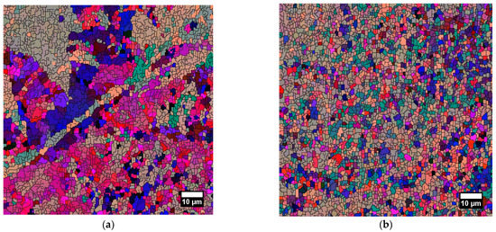
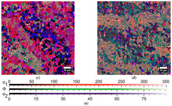
Figure 7.
Distribution maps of the Euler angles φ1, Φ, and φ2 of samples (a,b) C7-1 (near the C7 wire fracture region) and (c,d) C7-2 (far from the fracture region) in the center (a,c) and near the edge (b,d) of the cross-section. Euler angle legends and scales are shown in (e) with the same range of change in Φ and φ2.
In order to obtain quantitative characteristics of the microstructure of wires, an analysis of EBSD maps was carried out, which gave the number of grains of different sizes, the area occupied by grains of different sizes, and the number of grains with different misorientation angles between them.
For all samples of the C7 and C10 wires, Figure 8, Figure 9, Figure 10 and Figure 11 present the grain-size-distribution histograms (Figure 8), dependences of the relative area occupied by grains on their size (Figure 9), grain-aspect-ratio distribution histograms (Figure 10), and grain-boundary misorientation-angle distribution histograms (Figure 11) obtained from the analysis of EBSD maps. For samples C8-1 and C8-2, which are cut from the C8 wire destroyed under cyclic loading, the corresponding Figures are moved to Supplementary Materials (Figures S11–S13) since the histograms for these samples are qualitatively similar to the results obtained for the C7 wire (Figure 8a,b, Figure 9a,b, Figure 10a,b and Figure 11a,b) also failed during fatigue testing. For easier comparison, all histograms and plots in Figure 8, Figure 9, Figure 10 and Figure 11 and Figures S11–S13 are shown at the same scale. For the unused sample 5-2 from the A50 type cable and its AC50 counterpart, EBSD maps and data of their analysis are given in [21,22,23].
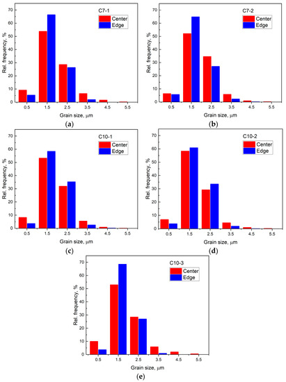
Figure 8.
Grain-size distribution histograms in the central and edge areas of samples: (a) C7-1 (near the C7 wire fracture region), (b) C7-2 (far from the fracture region), (c) C10-1 (from the region of the C10 wire near the 1st clamp), (d) C10-2 (from the center of the C10 wire), and (e) C10-3 (from the region of the C10 wire near the 2nd clamp). For better visualization, the histograms are shifted along the abscissa axis by the width of the base of the histogram columns to the left and right relative to the true position.
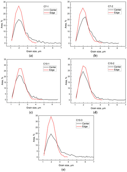
Figure 9.
Dependences of the relative area occupied by grains on their size in the central and edge regions of samples (a) C7-1 (near the region of destruction of the wire C7), (b) C7-2 (far from the region of destruction), (c) C10-1 (from the area of the C10 wire near the 1st clamp), (d) C10-2 (from the center of the C10 wire), and (e) C10-3 (from the area of the C10 wire near the 2nd clamp).
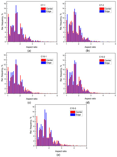
Figure 10.
Histograms of the distribution of the aspect ratios of grains in the region of the center and edge of samples (a) C7-1 (near the region of destruction of the wire C7), (b) C7-2 (far from the region of destruction), (c) C10-1 (from the region of the C10 wire near the 1st clamp), (d) C10-2 (from the region of the center of the C10 wire), and (e) C10-3 (from the region of the C10 wire near the 2nd clamp). For better visualization, the histograms are shifted along the abscissa axis by the width of the base of the histogram columns to the left and right relative to the true position.
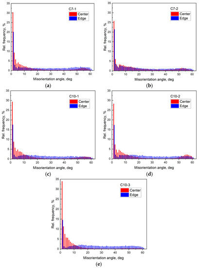
Figure 11.
Histograms of grain-boundary misorientation-angle distribution in the region of the center and edge of samples (a) C7-1 (near the C7 wire fracture region), (b) C7-2 (far from the fracture region), (c) C10-1 (from the region of the C10 wire near the 1st clamp), (d) C10-2 (from the region of the center of the C10 wire), and (e) C10-3 (from the region of the C10 wire near the 2nd clamp). For better visualization, the histograms are shifted along the abscissa axis by the width of the base of the histogram columns to the left and right relative to the true position.
One can see from the comparison of the plotted grain-size-distribution histograms (Figure 8 and Supplementary Materials Figure S11) with those for the unused sample before cyclic fatigue testing [21,22] that in all parts of all (C7, C8, and C10) wires, a slight increase is observed (from ~1% to ~5%) in the number of grains with a small size of ~1.5 μm and less and of a corresponding decrease in the number of grains of a larger size. Compared to wires after operation for 10 years or more, in wires after fatigue testing under different loads, there is a noticeable growth of grains with sizes less than ~3 μm, by ~1–15% for different grain sizes and samples, accompanied by a corresponding decrease in the number of large grains. As a rule, for wires after fatigue tests, the number of grains with sizes ~1.5 μm is noticeably larger at the edges compared with the centers of the cross-sections. The largest difference of ~18% between the edge and the center is observed for the C10-3 sample cut from the area near the 2nd (fixed) clamp of the wire not failed during testing. On the contrary, in the wires after operation [22], the edges and centers of the cross-sections differ little in grain size. Moreover, unlike the case of wires from cables after operation, grains larger than ~3.5 μm generally disappear at the edges of all samples after cyclic testing, although remaining in smaller quantities in the centers of their cross-sections. As a result, after fatigue testing, the grains have sizes of ~0.5–5.5 μm in the center and ~0.5–3.5 μm in the region of the edge of the wire cross-section.
In terms of average grain sizes Dgrain, the following changes are observed as illustrated in Supplementary Materials Figure S15. Yet, it should be noted in advance that the difference in Dgrain values between the new sample and the samples after fatigue tests is not impressive, since fatigue tests lead to a small change (1–15%) in the number of grains with small (< 3 microns) and large sizes, and averaging occurs over all grains with sizes from 0.5 microns to 5.5 microns. Nevertheless, some systematic changes in the average grain sizes are seen. After fatigue tests for wires fractured during testing, samples C7-1, C8-1 and C7-2, C8-2 cut from places both near and far from the break show the larger values of Dgrain (1.88–2.00 μm) in the centers of the wire cross sections and smaller Dgrain at the edges (1.72–1.76 μm). It is similar to the new sample 5-2 (1.92 μm and 1.78 μm, respectively) but with a slightly larger spread between the Dgrain values in the centers and at the edges, which is larger for the samples C8-1 and C8-2 tested with a larger maximum load σmax = 150.7 MPa. On the contrary, in the wires after operation, the Dgrain values in the centers and at the edges are practically the same as estimations show (1.98 μm both in the center and at the edge for wire from A50 type cable after 10 years of exploitation in OPLs (sample N8 in [21,22,23]) and 1.75 μm in the center and 1.76 μm at the edge for the wire after 20 years operation in an OPL cable of AC50 type (sample N6 from [22]). For wires not brought to fracture during fatigue testing, sample C10-3, cut from a position near a fixed clamp, shows markedly different values of Dgrain in the center of the cross section and at the edge (1.88 μm and 1.75 μm, correspondingly), similar to the samples cut from fractured wires. At the same time, samples C10-1 (cut from the area near the moving clamp) and C10-2 (from the middle of the wire far from the clamps) showed close Dgrain values in the centers of the cross-sections and at the edges (respectively, 1.89 μm and 1.87 μm for C10-1 and 1.85 μm and 1.84 μm for C10-2), similar to how it was observed for wires after operation.
The relative area Srel occupied by grains for samples after cyclic fatigue testing with different loads (Figure 9 and Figure S12 (Supplementary Materials)) shows a maximum at grain sizes of ~2.0–2.5 μm, reaching ~18–27.5% and ~27.5–34% for edges and centers of cross-sections, respectively. The difference in the maximum value of Srel at the edges and in the center ranges from ~5% (sample C10-2 from the middle of unbroken wire) to ~18% (for sample C10-3 from the area near the 2nd clamp of unbroken wire). An unused sample and wires from A50-type cables after operation without a short circuit for 10–62 years also show a maximum Srel at grain sizes of ~2.0–2.5 μm with a value of ~26% and ~18–20% for the centers of the cross-sections of the samples [21,23], i.e., ~1.3–1.9 times less than for wires after fatigue tests.
The aspect ratio for all samples has a value from 1 to 5. Its general appearance for an unused sample and wires after operation in OPLs [23], as well as after cyclic tests at different loads, changes slightly in the center and at the edges of the cross-section (Figure 10 and Figure S13 (Supplementary Materials)). There are some exceptions, e.g., scattered deviations of ~1–2% of the relative-frequency value in the center and at the edge of the samples after operation and after fatigue tests for some aspect ratios less than the value equal to 2. The greatest difference is once again shown by samples C10-3 from the region near the 2nd clamp of unfractured wire, in which the relative frequency of grains with the aspect ratio of 1.6 and 1.7 is ~4% higher at the edge than at the center. Nevertheless, the similarity of the shapes of aspect-ratio histograms in the center and at the edges of the cross-sections of the samples before and after fatigue tests and after operation in power transmission lines indicates the invariability of the grain shape, at least in the first approximation.
In the distributions of misorientation angles φmis of grain boundaries in the center of samples after fatigue testing (Figure 11 and Figure S14 (Supplementary Materials)), low-angle (φmis ≤ 15°) boundaries dominate, characterized by a bell-shaped distribution function of φmis with a maximum at φmis = 2°, and a local bell-shaped maximum is observed in the region of φmis = 50–60°. The same form of distribution of the misorientation angle of grain boundaries in the region of the center and edge of the cross-sections of the wires, although with different numerical characteristics, is typical for the sample before testing and for the wires after use in cables of power transmission lines [22,23]. The relative frequency of repeatability of low-angle (value at maximum at φmis = 2°) and high-angle boundaries at φmis = 50–60° in samples after fatigue testing is ~26–34% and ~0.5–2.0%, respectively, in comparison with ~22% and ~2.5% for the sample before testing [22,23]. A similar increase in the number of low-angle boundaries up to ~28–31%, accompanied by a decrease in the number of high-angle boundaries down to ~0.4–1.2% at the centers of wire cross-sections after operation in A50 cables during 10–62 years, was associated in [21,22,23] with a tendency for the orientation of crystal lattices of grains to align along a common direction. Such a tendency to equalize the grain orientations along a common direction also takes place in wires after fatigue tests.
In Al wires from used A50-type cables, the tendency to align the grain orientations is the same throughout the wire but is more pronounced at the edges of the wire cross-sections than at the centers. However, in contrast, in the region of the edge of the samples after fatigue testing, the distribution has a uniform character in the form of an almost horizontal line at all misorientation angles φmis, with a relative frequency of about 3–4% without pronounced maxima, except for a delta-shaped peak with a relative frequency of ~15–25% at φmis = 2°. Probably, such a distribution of misorientation angle φmis of grain boundaries is the result of a specific grain distribution, when about 15–25% of neighboring grains at the edge of the wires after fatigue tests lined up rather well along a direction, forming clusters of grains of similar colors on EBSD maps (Figure 7 and Figures S9 and S10 of Supplementary Materials), while the rest of the grains are randomly and uniformly misoriented relative to the grains in these clusters.
Thus, the EBSD study of Al wires from A50 (AAAC)-type cables after cyclic fatigue tests shows that the microstructure of these wires differs from the microstructure of Al wires from A50 cables that served without a short circuit in OPLs under natural conditions.
3.4. Results of Fractographic Analysis of the Samples C7 and C8 Ruptured during Cyclic Fatigue Tests
Finishing the characterization of the microstructure of the samples, in order to obtain information about the type of fracture surface and the mode of fracture of aluminum wires during fatigue tests, let us consider the results of fractographic analysis of samples C7 and C8 that were ruptured as a result of fatigue tests.
Fractographic analysis performed using SEM images (Figure 12a,b) shows that the fracture surface of sample C7 has a V-shaped type, whereas for sample C8, it is quasi-planar. Both types of the fracture surface have been recently observed [2,4,5,7,10] for Al wires from AAAC and ACSR cables after the fatigue tests.
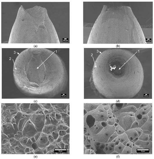
Figure 12.
SEM images of the Al-wire samples (a,c,e) C7 and (b,d,f) C8 in the place of their rupture after the fatigue tests, taken laterally and frontally. Fractographic analysis of SEM images reveals different zones indicated in (c,d) by numbers, corresponding to, respectively, fibrous (1), radial (2), and cut (3) zones of the fracture surface. White spots on (d) are contamination on the surface.
Another feature revealed during the fractographic examination is the formation of three different zones on the fracture surface, indicated in Figure 12c,d and Figure S16a,b (Supplementary Materials) by numbers. The cut zone 3 near the edge of the rupture is rather smooth and small. At the same time, the radial zone 2 contains radial scar formations corresponding to propagation of fatigue cracks. It is difficult to determine where zone 3 ends and zone 2 begins as there is no distinct border. However, the scar traces characteristic of the radial zone found upon careful examination of the SEM images seem to indicate that zone 2 is larger than zone 3 in both samples. Probably due to the significantly greater number of tensile-relaxation cycles for the C7 sample during fatigue testing (Table 1), this sample is characterized by a significantly (~10 times) larger area of fibrous zone 1 compared to the C8 sample (cf. Figure 12c,d). The radial zone 2 of the fracture surface in the wire C7 is correspondingly smaller than in C8.
SEM images in Figure 12e,f show the fibrous zone 1 on a larger scale (slightly larger scales are shown in Supplementary Materials Figure S16c–f). The fibrous zone 1 contains fibrous formations (fatigue striation marks), as well as dimples (with pores) characteristic of a quasi-viscous fracture regime, as indicated in [38], where a similar microstructure (dimples with pores) of the fracture surface was found for a microcrystalline aluminum alloy.
3.5. Elastic and Microplastic Properties
The elastic and microplastic properties of aluminum wires were determined by the resonance method of a composite piezoelectric vibrator. Figure 13 shows the amplitude dependences of Young’s modulus E(ε) and decrement δ(ε) for samples after fatigue testing. Here, ε is the amplitude of the vibrational deformation of the sample, which is a measurable quantity alike the decrement δ. Young’s modulus (modulus of elasticity) was obtained according to [39] (see Supplementary Materials Section S2). The dependences E(ε) and δ(ε) were measured with an increase and subsequent decrease in the amplitude ε.
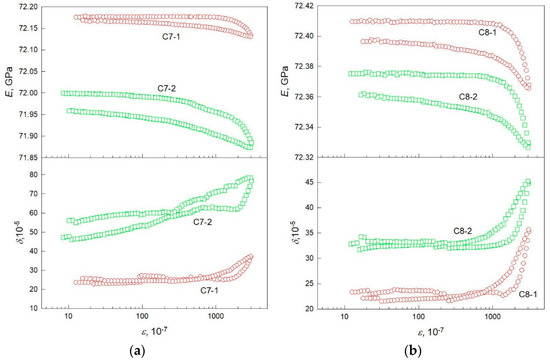
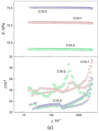
Figure 13.
Amplitude dependences of Young’s modulus E, and decrement δ of aluminum wires after fatigue tests for samples (a) C7-1 and C7-2, (b) C8-1 and C8-2, and (c) C10-1, C10-2, and C10-3. The measurements were made at the room temperature.
Figure 14 shows acoustic-strain diagrams σ(εd) for specimens after fatigue testing, plotted using the dependences E(ε) and δ(ε) of Figure 13, taken with the increase in amplitude ε, which was carried out first. Along the ordinate axis in Figure 14, the vibrational-stress amplitude σ (obtained from Hooke’s law, see Supplementary Materials Section S2) is plotted, and along the abscissa axis, the non-linear inelastic deformation εd is given. The values of E (= Ei), δi, and conditional micro-flow strain σs for sample 5-2 before testing [21] are given in Table 2, which also contains these quantitative parameters for all specimens after fatigue testing.
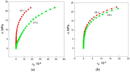
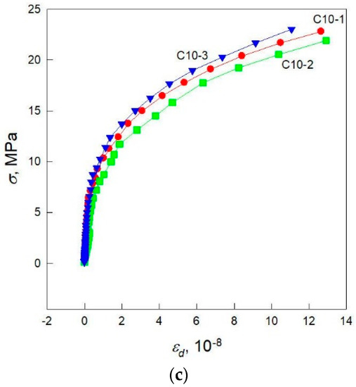
Figure 14.
Diagrams of microplastic deformation of aluminum wires after fatigue testing for samples (a) C7-1 and C7-2, (b) C8-1 and C8-2, and (c) C10-1, C10-2, and C10-3. The measurements were made at the room temperature.
Table 2.
Young’s modulus E, amplitude-independent decrement δi, and conditional micro-flow strain σs at inelastic deformation εd = 1.0 × 10⁻⁷.
The change in elastic and microplastic properties after fatigue tests relative to the initial sample (sample 5-2) seems natural. Obviously, during cyclic loading, the dislocation density in the wires increases; according to the theory of internal friction, this leads to a decrease in the Young’s modulus E and an increase in the decrement δi. In addition, the densitometry measurement of the integral density ρ of wire samples showed that after fatigue tests, a negative density defect Δρ/ρ (decrease in density, see Figure 2) is formed in the samples relative to the initial sample 5-2, and it also leads to a decrease in the modulus. Thus, in sum, the decrease in the modulus for samples C7 and C8 is natural. For the specimen C10 not brought to failure during fatigue testing, the elastic modulus E increases or decreases relative to the initial state (depending on the specific part of the specimen), as can be seen from Figure 13c. Its smallest value E = 71.83 GPa corresponds to the central part of the C10 wire (C10-2 sample), far from both clamps. Note that in the initial state (before testing), Young’s modulus E was 72.78 GPa (Table 2).
One can see from Figure 13a,b that the patterns of the dependences E(ε) and δ(ε) for both samples of C7 and C8 wires failed during cyclic loading are identical. There are only differences in the absolute values of the elastic-plastic characteristics of the samples (cf. Table 2) and they are most likely due to the different deformation prehistory of these samples. For the Young’s modulus E(ε) and the decrement δ(ε) in the samples of C7 and C8 wires brought to failure, amplitude hysteresis is observed, i.e., the E(ε) and δ(ε) curves taken with an increase and subsequent decrease in the amplitude do not coincide. Furthermore, for samples C7-1 and C8-1 located closer to the area of destruction, which occurred at a distance of ~15–20 mm from the movable clamp 1 (Figure 1), the values of Young’s modulus E are higher, and the decrement δ is lower than for samples C7-2 and C8-2 cut from a remote undamaged area near another clamp. For sample C7-1, the value of the modulus E is higher although the integral mass density ρ is noticeably lower according to the densitometric measurements of this part of the wire (by 0.13% relative to C7-2, see Figure 2 and Supplementary Materials Table S1), which should lead to a lower value of the modulus E. When analyzing the data, it is important to take into account that the value of the elastic modulus E is also affected by long-range fields of high internal strains. Thus, the density of dislocations obviously increases in the process of plastic deformation under cyclic loading. The local accumulation of dislocations becomes possible, which in turn can lead to the formation of long-range internal-strain fields and, as a result, to a higher Young’s modulus E. It is also obvious that such local formations (their higher concentration as sources of internal strain) are the most probable just in the region near the future fracture; that is why the Young’s modulus E of sample C7-1 cut from the region near fracture is somewhat higher than in the case of sample C7-2 from a part of the wire remote from the destruction region. A similar behavior is also observed for samples C8-1 and C8-2; that is, parts of the C8 wire near and far from the fracture region, respectively. The assumption about high internal-strain fields is consistent with a rather high value of microstrains εs detected by the WHP and SSP methods when analyzing the broadening of XRD reflections for samples of C7 and C8 wires brought to failure (Supplementary Materials Table S2, Figure 6).
The amplitude-independent decrement δi is proportional to the density of dislocations (the higher the dislocation density, the higher the total decrement δ). According to the obtained data (Table 2 and Figure 13a,b), the decrement in the areas near the fracture sites (samples C7-1 and C8-1) is lower than in the other parts of the wires, C7-2 and C8-2. To understand the reason for this, let us turn to the EBSD microstructural data on grain size distributions for the initial, unused sample 5-2 [21,22] and samples C7-1 and C8-1 from areas near the wire fracture after fatigue testing (Figure 8a and Figure S11a). Since the qualitative data for both samples after cyclic fatigue tests with different maximum loads are the same, let us take for certainty the data for the sample C7-1 with maximum cyclic load σmax = 149.4 MPa. It follows from the obtained distributions that after fatigue testing, the number of grains with sizes up to 1 μm increases from ~5% in the original sample to ~10% in the center of sample C7-1, whereas the proportion of grains with sizes 1–2 μm decreases from ~58% to ~54%. Smaller grains (subgrains) can indeed be formed during plastic deformation in the course of cyclic tests in the area located near the fracture. They contain quite a few dislocations inside, and it causes a decrease in the average dislocation density. Sample C8-1, which is also cut from an area near the fracture site, shows similar changes in grain sizes after cyclic fatigue testing with a higher load σmax = 150.7 MPa, though with somewhat different quantitative values, namely the number of grains in the center of the sample with sizes up to 1 μm is ~7% and the proportion of grains with sizes 1–2 μm is ~51%. Apparently, it is exactly such structural changes in grain sizes that lead to a decrease in the decrement δi in C7-1 and C8-1 in this case.
For wire C10, which was not brought to a fracture during cyclic fatigue testing at the even higher load σmax = 155.9 MPa, the values of the amplitude-independent decrement δi differ insignificantly depending on the place of sample cutting (Table 2), even coinciding for samples C10-1 and C10-2, which may indicate approximately the same structural state (dislocation density, grain size, etc.). In addition, for these C10-1 and C10-2 samples, one can note the presence of small maxima of the total decrement δ with an increase in the amplitude of vibrational deformation ε and their absence with a successive decrease in this deformation (Figure 13c). Such a behavior of the decrement may be due to the presence of any stoppers (defects, dispersed particles, etc.). At the same time, Young’s modulus E shows (see Figure 13c, Table 2) the greatest difference among the samples cut from different locations of the C10 wire. This modulus E is maximum for sample C10-3 from the region near the fixed clamp 2 (Figure 1), somewhat less for sample C10-1 from the region near the other clamp (clamp 1, movable during fatigue test), and minimum for sample C10-2 from the area of the middle of the wire far from both clamps (respectively, E = 73.00 MPa, 72.59 MPa, and 71.83 MPa compared to 72.80 MPa for the initial sample 5-2 before fatigue testing).
Let us next analyze the diagrams of plastic deformation σ(εd) shown in Figure 14. The strongest difference can be noted between samples C7-1 and C7-2, the values of the conditional micro-flow strain σs differing almost twice (Table 2). In addition, an analysis of the σ(εd) dependences for C7-1 and C8-1 shown in Figure 14a,b, respectively, reveals that the micro-flow strain increases as the fracture area is approached. As noted above, a certain decrease in the average grain size is observed in the fracture area due to the formation of subgrains inside the grains, which causes the higher value of σs. Another hardening factor is a significant increase in the dislocation density during long-term tests in the fatigue loading mode. Note that the highest value of the conditional micro-flow strain among all the studied samples is observed in the C10-3 sample from the area of the fixed clamp 2, namely σs = 23 MPa compared to 21 MPa for the C10-1 sample near the movable clamp 1 and 20 MPa for the sample cut from the middle of the wire away from both clamps.
4. Discussion
Our studies of single wires of AAAC cables (A50 type) after laboratory cyclic fatigue tests, which were carried out by densitometry, XRD, EBSD, and with acoustic measurements, have revealed not only the parameters of their structure, microstructure, and elastic-plastic properties, which change in a way similar to that after the operation of these wires in cables of OPLs in natural conditions, but also the parameters with different a response.
4.1. Mass Density of Al Wires after Fatigue Testing According to Densitometry and XRD Investigations
Densitometric measurements (Section 3.1) and XRD studies (Section 3.2) have shown that after fatigue tests, as well as after the use of wires in the OPL cables [21,22,23], there is a decrease in both the integral mass density of the wires ρ and in the XRD mass density ρX of their NSL with a thickness of ~36 μm (Figure 2 and Figure 5b), probably due to the formation of defects of a void nature in the wires, first and foremost in their NSL. Moreover, this decrease in ρ and ρX is different for different parts of the wires, namely the drop of both densities is stronger for the wire parts close to destruction positions near the grips holding the wires during cyclic fatigue testing. The drop in the XRD mass density, ρX, is caused by the lattice expansion (increase in the parameter a of the cubic unit cell (Figure 5a)) of the Al material of wires, apparently due to the stretching of the wires during cyclic fatigue tests by loading-relaxation according to a sinusoidal law and, as suggested above, owing to the formation of defects of the void nature in NSL. Probably, the same reasons lead to a decrease in the integral density ρ of the tested wires, though to a lesser extent, that is why the values of ρ are close to the values of the XRD density ρX, although slightly smaller. In addition, aluminum oxides are not formed in NSL of wires after fatigue tests, whereas these oxides with a higher mass density than that of pure Al were detected in [21,23] by means of XRD studies of NSL of wires from OPL cables with different service lives in natural conditions. As a result, there is no increase in the value of the integral density ρ of the entire wire due to the absence of more dense Al oxides in NSL of tested wires.
4.2. Effective Service Life of Al Wires after Fatigue Testing
Upon studying the wires from A50-type cables of OPLs with a service life of up to 20 years, it has been found out by [23] that the parameter a of the cubic unit cell of the Al material of the NSL of wires with a thickness of ~36 μm linearly increases at a rate of vcor = 1.26(4) Å/year, and its X-ray mass density ρX, correspondingly, linearly decreases at a rate of vcor = 2.52(8) g/cm3/year (vcor is called “corrosion rate” in [23]). Table S2 in the Supplementary Materials presents the values of the effective service life teff of the samples, estimated from their XRD density ρX as , where ρX0 is XRD mass density of unused sample 5-2 (the analogous estimates of teff from the parameter a do not differ up to values after the decimal separator). For ease of comparison, the values of the effective life teff of the samples are also shown graphically in Figure 15 as a function of ρX. The exactly linear decline of teff(ρX) is simply the result of using a model of linear X-ray-density drop as service life increases, as described above.
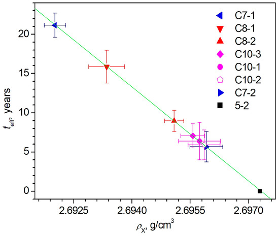
Figure 15.
Effective service life teff of wire samples C7, C8, and C10 after fatigue testing and that of a new sample 5-2 before testing as a function of the density ρX of the samples, estimated from XRD.
It should be noted that the “effective life” teff of the wires is not the real service life, but one to which the state of the wire corresponds (according to the previous calibration) as a result of operation. The value of teff can obviously differ for different parts of the same wire, with “older“ parts of the wire being the candidates for earlier destruction.
The C7-1 and C8-1 samples, cut from regions near the positions where the wires failed (regions near non-fixed grip 1), show large values of teff ≈21 years and ≈16 years, respectively, in comparison with teff ≈5.5 years and ≈9 years for samples C7-2 and C8-2 from regions far from the sites of destruction; that is to say, the difference between the effective service lives of the parts of wires broken during testing decreases from ~15.5 years to ~5 years with an increase in the maximum load σmax of cyclic fatigue tests from 149.4 MPa to 150.7 MPa (see Table 1). In other words, for wires that failed during testing at a lower load of cyclic tests, parts of the wires near and far from the fracture region are farther in terms of effective service life (in terms of “age”) than under higher loads. to put this in simpler terms, the effective service lives (“ages”) of different parts of the failed wire far and near the fracture area converge with an increase in the load of cyclic tests.
The sample C7-1 from the region near the wire break after cyclic testing with the lowest applied load σmax = 149.4 MPa shows the maximum estimated value of teff, which is equivalent to ~21 years of service. This effective lifetime is less than half the expected lifetime of the A50-type cable, which is 45 years according to its datasheet [1]. The decrease in effective service life is obviously due to the fact that individual outer wires from the cable were subjected to fatigue tests but not the entire cable. For the C10 wire, which did not fail during cyclic fatigue testing, samples C10-1 and C10-3 from the regions near the grips and sample C10-2 from the middle of the wire far from the grips are characterized by only a small difference in teff (6.2(2.2), 6.9(1.5), and 5.7(1.8) years, respectively), nevertheless, the C10-2 sample from a location on the wire far from the grips does show the smallest value of teff.
4.3. Preferential Orientation of Crystallites (from XRD) and Grain Orientation Alignment (from EBSD) in Al Wires after Fatigue Testing
In addition to lattice expansion and the corresponding decrease in XRD density in NSL of wires, there is also an increase in the preferential orientation along the [011] crystallographic direction of the Al crystal lattice (Figure 4) in wires after fatigue tests (more correctly, in their NSL with a thickness of ~36 μm, which is tested by means of XRD), alike that in wires from OPL cables with different service lives [21,22,23]. The increase in the preferential orientation of the crystal structure of the wires correlates with the increase in the tendency to equalize the orientation of the crystal structures of the grains along a common direction, which was observed in the study of EBSD maps from the cross sections of the samples after the operation of the wires in OPL cables in natural conditions [21,22,23] and after fatigue tests (Section 3.3). Moreover, after operation in OPLs, this tendency of grain-orientation alignment along one direction is observed not only in the center but also at the edges of the cross-section of the samples, even though it is stronger at the edges, “the edge”, meaning the position of ~150 μm from the wire surface. It is important to recall that as a result of this observed trend in grain alignment, misorientation-angle histograms showed a gradual nonlinear increase in the number of low-angle grain boundaries with φmis < 15° and with a maximum at φmis = 2°, as well as a decrease in the number of high-angle boundaries in the region φmis = 50–60°, where there was a local wide maximum on the histogram.
Meanwhile, a similar picture as described above from the wires exploited in OPLs observed after fatigue testing in the center of the cross-sections of all samples (Figure 11 and Figure S14 (Supplementary Materials)), whereas at the edge of the cross-section of all wires after fatigue tests, the alignment of the grain orientation was almost complete. In the edges of all samples after fatigue tests, about 20–25% of grains had a very small misorientation of ~2°, while the rest were uniformly and randomly misoriented in all possible angles. As a result, the histograms of misorientation angles at the edge of the samples show a delta-shaped peak at φmis = 2° and a low number of grains uniformly distributed over all other φmis. Such a difference between the samples after operation in natural conditions and after laboratory cyclic fatigue tests is perhaps due to the fact that the load under natural conditions does not vary uniformly over time; there are different types and directions of wires’ oscillations and vibrations depending on the wind strength, and, in addition, there is the influence of the changing temperature and humidity of the surrounding atmosphere, as well as that of electric current. Because of these influences, the grain alignment is not as ideal as in the case of laboratory tests with a constant sinusoidal law of loading and relaxation of the wires.
4.4. Size of Crystallites and Microstrains in Them (from XRD) and Size of Grains (from EBSD) in Al Wires after Fatigue Testing
An important difference between wires after natural service and after fatigue testing in the laboratory is the size of their crystallites (obtained from XRD studies) and grains (from EBSD). Crystallites (regions of coherent X-ray scattering) are regions of parallel atomic planes without misorientation. Their sizes are determined from the analysis of XRD reflection profiles (for example, by WHP or SSP methods, as in Section 3.2) and usually range from 2–5 nm to 200–300 nm, i.e., XRD characterizes microstructures with sizes under ~0.3 μm. EBSD, on the contrary, characterizes the sizes of large microstructure objects, namely from ~0.5 μm to tens–hundreds of microns, which are called grains. The crystal structure of these grains is not as ideal as that of crystallites. Grains can contain many crystallites, the crystal lattices of which are slightly misoriented relative to each other. In the present study, for example, regions were considered as grains when their crystal structure was misoriented by less than 2°.
Previously [21,22], it has been found for wires made of A50 cables of AAAC type with different service lives that, after operation in OPLs for 10 years or more, the crystallite sizes D increase from ~110 nm in unused Al wire to ~250–300 nm in a wire after operation, with microstrains in them simultaneously appearing, εs ≈ 0.030–0.034%. At the same time, the analysis of EBSD maps shows that in the center and at the edges of the wire cross-sections, the number of small grains with sizes of less 3 µm decreases while the number of large grains with sizes 3.5–5.5 µm increases. As a result, the average grain size Dgrain in the centers and at the edges become almost the same (for example, ~1.98 µm in the wire from the A50 cable after 10 years of operation in OPL (sample N8 in [21,22,23])), unlike the new unused sample (Supplementary Materials Figure S15).
On the contrary, for wires after cyclic fatigue tests, the pattern of changes in the microstructure is different on both scales. Microstrains in crystallites after fatigue testing are at approximately the same level (εs ≈ 0.022–0.034%) as for wires after operation in OPLs and are formed in all parts of the wires broken during fatigue testing as well as in parts of the intact C10 wire close to grips, or at least to fixed grip 2 (Figure 1). The crystallite sizes show an increase to lesser values D ~145–180 nm and only for parts of the failed C7 wire (Supplementary Materials Table S2) subjected to cyclic fatigue testing with the lowest maximum load σmax = 149.4 MPa. At higher loads, the crystallite sizes, on the contrary, sequentially decrease to D ~90–100 nm and ~60–106 nm at σmax = 150.7 MPa (samples C8-1 and C8-2) and σmax = 155.9 MPa (samples C10-1, C10-2, and C10-3), respectively. In the center and at the edges of samples after fatigue testing, in contrast to samples after operation, the number of small grains (< 3 μm; and, in particular, the number of smaller grains with sizes of <1.5 μm) increases and the number of large grains with sizes of >3.5 μm decreases in centers of the cross sections of the samples and completely disappears at the edges. As a result, for the samples after fatigue tests, the average grain size Dgrain in the centers changes in the limits of about −2–4% (1.88–2.00 μm), and at the edges decreased by ~1–2% down to 1.72–1.76 μm compared to the corresponding values of 1.92 μm and 1.78 μm in the new sample (Supplementary Materials Figure S15).
Thus, for samples that served under natural environmental conditions, there is the size enlargement of microstructure objects, both on size scales less than 0.3 μm (crystallites, according to XRD results) and on large scales (grains). In contrast to natural conditions, a reduction in size of the crystallites and grains was observed in laboratory fatigue tests. The difference is again probably due to the difference in conditions in nature and in laboratory tests. The formation of subgrains (an increase in the number of grains of small size) was observed during plastic deformation of wires as a consequence of laboratory cyclic fatigue tests by loading–relaxation of the wires according to a sinusoidal law, remaining invariable during the tests. In natural operating conditions, it is necessary to take into account the temperature (current flow through the conductor, atmospheric conditions). For aluminum wire (for the manufacture of which A7E grade aluminum is used of technical purity 99.70 wt.% Al [35]), this temperature is sufficient for the process of grain increase of Al wires to occur during a typical exploitation time (decades) of OPLs’ cables.
In OPLs, the main mechanical load on the wires in exploiting OPLs is due to fretting and bending of cables under the influence of wind. In this case, the friction energy of the wires against each other or the friction of microstructural elements inside the wire (grains, subgrains, i.e., crystallites as well) is converted into internal energy, which leads to energy dissipation and local heating. Crystallites fuse together thus increasing in size, D ~110 nm to D ~250–300 nm. The same thing happens with grains. The number of small grains with sizes of less 3 µm decreases while the number of large grains with sizes 3.5–5.5 µm increases. The misorientation of the grains naturally decreases in this case.
Another possible reason for the growth of crystallites and grains in the Al wires after operation in OPLs is recrystallization due to influence of an electrical current in the conductor cables of OPLs under high voltage. The thickness of the NSL through which the current mainly flows is from ~ 0.057 mm to 0.18 mm [22]. Because of this, EBSD shows both an increase in the number of large grains with sizes 3.5–5.5 µm mainly in the edge region (i.e., in NSL) of the cross-sections of the wires after operation in OPLs [22,23] and the absence of large grains in NSL wires after fatigue tests that were not operated in high-voltage OPLs.
In fatigue tests, loading-relaxation is again converted into heat due to the scattering of collective vibrations of atoms on structural inhomogeneities. The test load σmax ~150 MPa at Young’s modulus of aluminum E ~ 70 GPa = 70,000 MPa gives the maximum strain in crystallites εs max = 150/70,000 ≈ 0.002 = 0.2% (residual microstrain εs determined from XRD data is an order of magnitude less). This quite high, and the heated microstructural elements (grains) begin to “melt” and become pulled apart by the applied force, crushed into smaller sizes such as drops, i.e., the size of the grains here, on the contrary, decreases. Thus, due to the absence of fretting and the effect of the electric current, large grains (and crystallites) are not formed after fatigue tests but small grains appear, caused by the effects of tensile loading-relaxation cycles.
4.5. Elastic-Plastic Properties of Al Wires after Fatigue Testing
The elastic-plastic properties of Al wires of A50 cables after operation in OPLs [21,22,23] and Al wires of A50 cables that failed after cyclic fatigue tests (Section 3.5) show a qualitatively identical change for Young’s modulus E and amplitude-independent decrement δi, namely there is a decrease in the values E and increase in the δi in comparison with the unused wire (see Table 2).
As stated in Section 3.5, higher values of Young’s modulus E of the C7-1 and C8-1 samples from close-to-fracture regions of the relevant wires compared to samples taken far from the fracture region (C7-2 and C8-2) can be explained by the occurrence of fields of high internal strains, which arise due to the accumulation of dislocations formed during plastic deformation of the wires under cyclic loading, mostly in the regions near the fracture of the wires. This assumption is consistent with the formation of microstrains in crystallites, which was detected by the WHP and SSP methods from the analysis of the broadening of the XRD reflections. The decrease in the decrement δi in samples C7-1 and C8-1 compared, respectively, to C7-2 and C8-2 can be explained by a lower dislocation concentration due to the fact that, according to EBSD studies, smaller grains with sizes less than 1 μm, in which there are fewer dislocations, are formed predominantly in regions near the fracture positions (Figure 8a,b and Figure S11 in Supplementary Material).
A decrease in the average size of grains (and of crystallites) and an increase in the dislocation density also lead to an increase in the conditional micro-flow strain σs of the wire material for most samples compared to the unused sample (from 18 MPa in the unused 5-2 sample to 19–22 MPa in other samples, see Table 2), i.e., to the opposite effect compared to the influence of the operation of wires in natural conditions, where a decrease in σs is observed (down to 2.3–13.1 MPa for Al wires from A50 cables with a service life of 10 to 62 years [21]). It is possible that the C10 wire, which did not fail after fatigue test with the highest maximum load σmax = 155.9 MPa, remained intact because this wire is characterized by an increased number of grains with small grain size < 1 μm and smaller crystallite size compared to other wires tested with lower loads (Figure 8 and Supplementary Materials Table S2). For the same reason, the value σs = 20–22 MPa is higher for its parts than that for other samples. Sample C7-2 (the C7-wire part far from the fracture site) is an exception in terms of change in the conditional micro-flow strain σs. The σs value in this sample drops down to 10 MPa, which is explained by the fact that in this sample, the number of small grains with sizes < 1 μm practically does not change in comparison with the unused sample (compare Figure 8b and Ref. [21]). In the C8-2 sample (the C8-wire part far from the fracture region), the number of small grains with sizes < 1 μm is approximately the same as in C7-2 (~5–6% in the center and at the edges of the cross-section); however, in comparison with C7-2, the number of grains of likewise small though slightly larger, with a size of ~2.5 μm, increases (from ~37% in C8-2 compared to ~34% in C7-2 for the centers of cross-sections). As a result, for sample C8-2, the value of σs increases to 19 MPa.
4.6. Prediction of the Location of a Break in an Al Wire That has Not been Brought to a Rupture during a Fatigue Testing
Let us now compare the characteristics of different parts of the C10 wire not brought to failure during fatigue testing and parts of the C7 and C8 wires that failed (broke) during testing.
Samples C7-2 (after fatigue testing with a maximum load σmax = 149.4 MPa) and C8-2 (σmax = 150.7 MPa) from regions of the wires remote from the rupture positions show some common characteristics that distinguish them from the samples from the rupture regions, C7-1 and C8-1, respectively. For example, samples C7-2 and C8-2 are characterized by larger integral and XRD densities (cf. mass densities ρ and ρX in Supplementary Materials Tables S1 and S2 and Figure 2 and Figure 5b), a smaller Al cubic-unit-cell parameter a (Supplementary Materials Table S2 and Figure 5a), larger crystallite size D for sample C7-2 and comparable though slightly smaller (within e.s.d.) size D for C8-2, and almost the same (C7-2 vs. C7-1) or smaller (C8-2 vs. C8-1) microstrain value εs (Supplementary Materials Table S2 and Figure 6a,b). The effective service life teff of these samples, C7-2 and C8-2, is noticeably less than that of samples from regions close to the fracture positions (Supplementary Materials Table S2 and Figure 15). In addition, the C7-2 and C8-2 samples (from regions of the wire far from the rupture) compared to C7-1 and C8-1 (from regions near the rupture) show a greater influence of the effects of preferential orientation along the Al [011] direction (Supplementary Materials Table S2 and Figure 4). Samples C7-2 and C8-2 at the cross-section center show fewer small grains with sizes < 1 μm compared to samples C7-1 and C8-1 (Figure 8a,b and Figure S11) and a smaller difference between the values of Srel (relative areas occupied by ~2 μm grains) at the center of the wire cross-section and at its edge (Figure 9a,b and Figure S12 (Supplementary Materials)). In terms of elastic-plastic characteristics, samples C7-2 and C8-2 compared to samples C7-1 and C8-1 are characterized by a lower Young’s modulus E and a larger value of the amplitude-independent decrement δi (Table 2). As for the value of the conditional micro-flow strain σs, it is, as noted above, a characteristic that depends on the parameters of the microstructure, and, depending on them, can take on both larger and smaller values.
The C10-2 sample from the center of the intact C10 wire compared to the C10-1 and C10-3 samples from the regions near the clamps is characterized by slightly lower mass densities ρ and ρX and, accordingly, by a somewhat larger parameter a of the Al cubic unit cell (Supplementary Materials Tables S1 and S2 and Figure 2 and Figure 5a). The effective service life teff of sample C10-2 is less than that of samples C10-1 and C10-3 (Supplementary Materials Table S2 and Figure 15). Although the difference between these characteristics is quite small (within one–two e.s.d.s), it can be considered as an indication of the trend of decreasing ρ and ρX, smaller teff, and increasing parameter a in the case of C10-2 compared to C10-1 and C10-3. As for the average crystallite size D, sample C10-2 shows its greater (within e.s.d.) value compared to C10-1 but noticeably smaller than in C10-3 (Supplementary Materials Table S2 and Figure 6a,b). Unlike C10-1 and C10-3, there are no microstrains in C10-2 (εs = 0) as in the initial unused sample 5-2. The effect of preferential orientation of Al crystallites along [011] is greater in C10-2 than in C10-1 but less than in C10-3 (Supplementary Materials Table S2 and Figure 4). The C10-2 sample in the center of the cross-section, just as samples C7-2 and C8-2 from regions far from the fracture site, compared to C7-1 and C8-1 from regions near the fracture, is characterized by a smaller number of small grains with sizes < 1 μm in comparison with samples C10-1 and C10-3 from the areas near the clamps (Figure 8c–e) and by the smallest difference between Srel, the relative areas occupied by ~2-μm grains, in the center of the wire cross section and at its edge (Figure 9c–e). As for the elastic-plastic characteristics (Table 2), the amplitude-independent decrement δi of sample C10-2 appeared to be the same as δi of sample C10-1 but less than that of C10-3.
For most of the above parameters, sample C10-2 from the middle of the unbroken C10 wire, compared to samples from C10-1 and C10-3 from areas near the clamps, shows trends which are similar to those in samples C7-2 and C8-2 from areas far from the ruptures of corresponding wires. Perhaps, in the middle of the wire between the clamps, wherefrom sample C10-2 was cut, a break is less probable compared to the areas near the clamps.
Sample C10-3 from the region near clamp 2 fixed during fatigue testing, shows the longest effective service life teff = 6.9(1.5) years (Supplementary Materials Table S2 and Figure 15), the highest crystallite size D = 106.4(9) μm and microstrain εs = 0.034(3)% (according to SSP, Supplementary Materials Table S2 and Figure 6a,b) compared to teff = 6.2(2.2) years, D = 57(3) μm, and εs = 0.007(64)% in C10-1. The effect of preferential orientation of Al crystallites along [011] in sample C10-3 is also the largest (Supplementary Materials Table S2 and Figure 4). Furthermore, for C10-3, the maximum among all C10 samples numbers of small grains with sizes < 1 μm in the center of the cross-section and with sizes ~2.5 μm at the edge of the cross-section are observed; the maximum number of large grains with sizes > 4.5 μm is also detected in the center of the cross-section of C10-3 (Figure 8c–e). Unlike samples C10-1 and C10-2, the average grain sizes Dgrain in the center and at the edge of the cross section of the sample C10-3 show, respectively, values 1.88 μm and 1.75 μm close to the observed Dgrain values in samples cut from wires that were fractured during fatigue tests (Supplementary Materials Figure S15). Additionally, the largest difference between the relative areas Srel occupied by grains with a size of ~2 μm in the center of the wire cross-section and at its edge (Figure 9c–e) was found for sample C10-3. Sample C10-3 is characterized by the largest Young’s modulus E = 73.00 MPa and the smallest decrement δi = 23 compared to E = 72.59 MPa and δi = 26 for C10-1.
The most likely location for sample C10 failure is located in the C10-3 part of the wire, near the rigidly fixed clamp 2. This is suggested, in general, by the analysis of the change in Young’s modulus E, decrement δi, and conditional micro-flow strain σs (from acoustic measurements), combined with densitometric data on a decrease in the total mass density ρ of wire samples, structural data (from XRD), an increase in the preferential orientation, an increase in the parameter a of the cubic unit cell, and an accompanying decrease in the X-ray mass density ρX of the near-surface layer of the Al material of the wire with a thickness of ~36 μm. Furthermore, it is also revealed by microstructural data on the change in the grain size in wires (from EBSD), on change in crystallite sizes D, and in the formation of local microstrains εs in crystallites (from XRD) after cyclic fatigue testing.
However, wires C7 and C8 failed in the area of the non-fixed clamp 1. Furthermore, in favor of a more likely wire break near the movable clamp, to which the load is applied, the propagation of phonons (collective displacements of atoms) along the wire is not instantaneous. As a result, the average displacements of the atoms are greater at a non-fixed clamp where a tensile load is applied, and it can lead to a break in the wire near this clamp. So, since the C10 wire was not brought to failure during fatigue testing, and its parameters might change as a result of further cyclic loading, a fracture is not excluded in the C10-1 position near the movable clamp 1 where the load was applied. Similarly, in [2,5,7,9], fatigue tests of cables have led to the conclusion that at the fatigue mark caused by small relative movement between the adjacent wires in the cable or between the cable and the clamp, cracks often occur, the formation of which can be reinforced by abrasive particles present in the clamps [5].
So, as a practical application of the results of the current experiments, the consideration of the structural, microstructural, and elastic-plastic properties of aluminum wires after fatigue tests leads us to the conclusion that in the wires of OPLs, the areas near the clamps are crucial for fracture. This cruciality of the areas near the clamps seems to be enhanced by the phenomenon of fretting when the cable oscillates, sways, or vibrates due to wind. Fretting was absent during fatigue tests in the current investigation, since they were carried out on single wires, rather than the whole cable.
5. Conclusions
Thus, according to the results of fractographic analysis, aluminum wires broken during single-wire tensile fatigue testing are fractured in a quasi-viscous mode.
Summing up, a comparison of the structural, microstructural, and elastic-plastic characteristics of Al wires from A50 AAAC-type cables shows that laboratory cyclic fatigue tests of single Al wires lead to qualitatively the same trends in parameter changes compared to the natural operation in OPL cables in the case of integral (ρ) and XRD (ρX) mass densities determined by densitometry and XRD methods, respectively. A decrease in ρ and ρX is observed due to both the stretching of the wires during either operation or testing and the formation of void defects, primarily in the NSL (near-surface layer) of wires with a thickness of about 36 μm. In accordance with the decrease in ρX, an increase in the parameter a of the cubic lattice of the Al material of wires was observed (XRD data). In addition, in laboratory tests just as during natural use, the preferential orientation of aluminum crystallites along the crystallographic direction [011] of the cubic Al lattice was enhanced (XRD), with microstrain εs appearing in the crystallites (XRD). Aspect ratios of grains, i.e., their shapes, practically do not change (EBSD data), with the relative area Srel occupied by grains (EBSD) also qualitatively remaining the same. In addition, after operation and after fatigue tests, qualitatively the same general trends of a decrease in Young’s modulus E and an increase in the amplitude-independent decrement δi were observed (in acoustic measurements), the magnitude of which, however, is significantly affected by the parameters of the microstructure of the samples.
The effective service life teff of the wire parts near the positions of rupture after fatigue tests, estimated from the XRD value of the mass density ρX of the wire NSL, was larger than for the wire parts away from the rupture regions. With an increase in the value of the maximum load σmax, the difference between the effective service life of different parts of a wire is reduced.
The operation of Al wires from A50 AAAC-type cables under natural conditions in OPLs and laboratory fatigue tests lead to significantly different wire microstructures, both at the scale of ~0.05–0.3 μm and at the scale of ~0.5–6 μm. After operation, enlargement of crystallites in Al wires occurs on a small scale, and an increase in the average grain size happens on a large scale [21,22,23]. After fatigue testing, the crystallite sizes either increase less or even decrease. On a large scale, this is accompanied by a decrease in the average grain size, caused by a noticeable increase in the number of small grains, probably as a result of plastic deformation of the wire during fatigue testing.
The microstructure at the center of the wire cross-sections and at their edges (at a distance of ~150 μm from the outer surface of the wires) differs after operation in OPLs and after fatigue tests. In wires after fatigue testing, the tendency of grain-orientation alignment in the centers of cross-sections is the same as either in the centers or at edges of cross-sections of the wires after operation in OPLs (by means of forming the grain clusters with a gradual non-linear increase in the number of grains as the misorientation angle φmis decreases from 15° to 2°), whereas at the edges, most grains (~25–35%) form clusters with a very small misorientation angle φmis = 2°, while grains with all other misorientation angles φmis are evenly and randomly distributed within these clusters. It is possible that such a type of microstructure is formed in wires during fatigue testing with a fixed cyclic sinusoidal law of wire loading and in the absence of random changes in the ambient atmosphere and temperature, as well as the absence of the influence of an electrical current.
Furthermore, the formation of aluminum oxides is not observed in the wires after laboratory cyclic fatigue tests, as happens after operation in OPL cables in natural conditions.
A comparison of the characteristics of parts of the wires after fatigue tests, which originated from areas near the fracture positions and far from it, with those of parts of the wire that did not fail during testing (near the clamps and far from them), has led us to the assumption that the properties of the wire parts near either of the wire clamps are crucial with respect to possible failure during fatigue testing.
Supplementary Materials
The following supporting information can be downloaded at: https://www.mdpi.com/article/10.3390/met13020298/s1, Section S1. Fatigue tests of samples: Figure S1. OM images of Al wire surface (sample 5-2), new condition (before testing); Table S1. Sizes (diameter d and length l) of cylindrical wire samples, which were cut from wires after cyclic fatigue tests for the XRD and acoustic studies, and their mass density ρ according to densitometric measurements; Figure S2. Photographs of a sample (a) in fatigue-test holders, (b) in the grips of the test equipment during the test, and (c) destroyed in the fatigue test; Section S2. Experimental details; Section S3. XRD results: Figure S3. XRD patterns from samples 5-2, C7-2, C8-1, C8-2, C10-1, C10-2, and C10-3; Table S2. Results of XRD analysis of wires from unused A50-type cables after cyclic loading; Figure S4. Comparison of XRD from samples in the 2θ-angle region near the Al 133 reflection after different stages of fatigue testing; Figure S5. Average sizes D0 of crystallites of the Al material of wires in the model of the absence of microstrains; Figure S6. WHP and (SSP plots for samples C7-1 and C7-2; Figure S7. WHP and SSP plots for samples C8-1 and C8-2; Figure S8. WHP and SSP plots for samples C10-1, C10-2, and C10-3 Section S4.EBSD: Figure S9. Maps of distribution of the Euler angles φ1, Φ, and φ2 for samples C8-1 (near the fracture region of the C8 wire) and C8-2 (far from the fracture region) in the center and near the edge (of their cross-sections.; Figure S10. Distribution maps of the Euler angles φ1, Φ, and φ2 of samples C10-1 (from the area of wire C10 near the 1st clamp), C10-2 (from the center of wire C10), and C10-3 (from the region of the C10 wire near the 2nd clamp) at the center and near the edge of the cross-section; Figure S11. Grain-size distribution-histograms in the region of the centers and edges of cross-sections of the samples C8-1 (near the region of destruction of wire C8), and C8-2 (far from the region of destruction); Figure S12. Dependences of the relative area occupied by grains on their size in the region of the center and edge of samples C8-1 (near the region of destruction of the wire C8) and C8-2 (far from the region of destruction); Figure S13. Distribution histograms of aspect ratios of grains in the region of the center and edge of samples C8-1 (near the region of destruction of wire C8), and C8-2 (far from the region of destruction); Figure S14. Histograms of grain-boundary misorientation-angle distribution in the region of the center and edge of samples C8-1 (near the wire fracture region C8) and C8-2 (far from the fracture region); Figure S15. Average grain sizes Dgrain in the centers and at the edges of the cross sections of the samples in dependence of maximum load σmax of cyclic tensile fatigue tests; Section S5. SEM images of the fracture surface of the C7 and C8 wires broken during the fatigue testing: Figure S16. SEM images of the Al-wire samples C7 and C8 in the place of their rupture after the fatigue tests, taken frontally; Abbreviations. References [21,22,23,27,25,30,26,24,33] are cited in the supplementary materials.
Author Contributions
A.A.L., Conceptualization, Investigation (XRD), Methodology, Validation, Project administration, Software, Data curation, Formal analysis, Visualization, Writing—original draft, Writing—review and editing; M.V.N., Conceptualization, Investigation (densitometry, acoustic), Methodology, Validation, Software, Visualization, Writing—original draft; A.I.L., Investigation (SEM, EDX, EBSD), Methodology, Software, Visualization, Writing—original draft; B.K.K., Investigation (acoustic), Methodology, Software, Visualization; A.G.K., Conceptualization, Investigation (acoustic), Methodology, Software; A.G.P., Writing—original draft, Writing—review and editing, Conceptualization; N.D.P., Data curation; Validation, Project administration; R.V.S., Conceptualization, Methodology, Project administration; P.N.B., Supervision, Conceptualization, Methodology, Funding acquisition; M.M.S., Conceptualization, Methodology; Resources; Funding acquisition; A.V.S., Conceptualization, Methodology; Resources; I.A.B., Conceptualization, Methodology; Resources; All authors have read and agreed to the published version of the manuscript.
Funding
This research was funded by the state assignment of Russian Federation FSWF-2020-0025 “Development of methods and analysis of ways to achieve a high level of safety and competitiveness of objects of energy systems based on digital technologies”.
Institutional Review Board Statement
Not applicable.
Informed Consent Statement
Not applicable.
Data Availability Statement
The data presented in this study are available on request from the corresponding author.
Acknowledgments
The work was carried out using the equipment and software of the Center of Joint Use “Materials Science and Diagnostics in Advanced Technologies” (Ioffe Institute, St. Petersburg, Russia).
Conflicts of Interest
The authors declare no conflict of interest.
Abbreviations
The list of abbreviations and symbols is given in Supporting Materials.
References
- Nakhimova, L.I. (Ed.) GOST 839-2019. Non-Insulated Conductors for Overhead Power Lines. Specifications; Strojizdat: Moscow, Russia, 2019. (In Russian) [Google Scholar]
- Fadel, A.A.; Rosa, D.; Murça, L.B.; Fereira, J.L.A.; Araújo, J.A. Effect of high mean tensile stress on the fretting fatigue life of an Ibis steel reinforced aluminium conductor. Int. J. Fatigue 2012, 42, 24–34. [Google Scholar] [CrossRef]
- Badibanga, R.; Miranda, T.; Rocha, P.; Ferreira, J.; da Silva, C.; Araújo, J. The effect of mean stress on the fatigue behaviour of overhead conductor function of the H/w parameter. MATEC Web Conf. 2018, 165, 11001. [Google Scholar] [CrossRef]
- Matos, I.M.; Rocha, P.H.C.; Kalombo, R.B.; Veloso, L.A.C.M.; Araújo, J.A.; Castro, F.C. Fretting fatigue of 6201 aluminum alloy wires of overhead conductors. Int. J. Fatigue 2020, 141, 105884. [Google Scholar] [CrossRef]
- Azevedo, C.R.F.; Henriques, A.M.D.; Pulino Filho, A.R.; Ferreira, J.L.A.; Araújo, A. Fretting fatigue in overhead conductors: Rig design and failure analysis of a Grosbeak aluminium cable steel reinforced conductor. Eng. Fail. Anal. 2009, 16, 136–151. [Google Scholar] [CrossRef]
- Rocha, P.H.C.; Langlois, S.; Lalonde, S.; Castro, F. A general life estimation method for overhead conductors based on fretting fatigue behavior of wires. Theor. Appl. Fract. Mech. 2022, 121, 103443. [Google Scholar] [CrossRef]
- Miranda, T.; Badibanga, R.; Araújo, J.A.; Silva, C.; Ferreira, J. Fatigue Evaluation of All Aluminium Alloy Conductors Fitted With Elastomeric and Metallic Suspension Clamps. IEEE Trans. Pow. Deliv. 2022, 37, 539–546. [Google Scholar] [CrossRef]
- Kalombo, R.B.; Martínez, J.M.G.; Ferreira, J.L.A.; da Silva, C.R.M.; Araújo, J.A. Comparative fatigue resistance of overhead conductors made of aluminium and aluminium alloy: Test and analysis. Procedia Eng. 2015, 133, 223–232. [Google Scholar] [CrossRef]
- Kalombo, R.B.; Reinke, G.; Miranda, T.B.; Ferreira, J.L.A.; da Silva, C.R.M.; Araújo, J.A. Experimental Study of the Fatigue Performance of Overhead Pure Aluminium Cables. Procedia Struct. Integr. 2019, 19, 688–697. [Google Scholar] [CrossRef]
- Rocha, P.H.C.; Díaz, J.I.M.; Silva, C.R.M.; Araújo, J.A.; Castro, F.C. Fatigue of two contacting wires of the ACSR Ibis 397.5 MCM conductor: Experiments and life prediction. Int. J. Fatigue 2019, 127, 25–35. [Google Scholar] [CrossRef]
- Levesque, F.; Goudreau, S.; Cardou, A.; Cloutier, L. Strain measurements on ACSR conductors during fatigue tests I—Experimental method and data. IEEE Trans. Power Deliv. 2010, 25, 2825–2834. [Google Scholar] [CrossRef]
- Said, J.; Garcin, S.; Fouvry, S.; Cailletaud, G.; Yang, C.; Hafid, F. A multi-scale strategy to predict fretting-fatigue endurance of overhead conductors. Tribol. Int. 2020, 143, 106053. [Google Scholar] [CrossRef]
- Zhou, Z.R.; Goudreau, S.; Fiset, M.; Cardou, A. Single wire fretting fatigue tests for electrical conductor bending fatigue evaluation. Wear 1995, 181–183, 537–543. [Google Scholar] [CrossRef]
- Zhou, Z.R.; Cardou, A.; Goudreau, S.; Fiset, M. Fundamental investigations of electrical conductor fretting fatigue. Tribol. Int. 1996, 29, 221–232. [Google Scholar] [CrossRef]
- Kul’kov, V.G.; Tyshkevich, V.N.; Kuryanov, V.N.; Sultanov, M.M.; Norov, D.S.; Narykova, M.V.; Kadomtsev, A.G.; Prasolov, N.D.; Brunkov, P.N.; Likhachev, A.I.; et al. Experimental studies of fatigue strength and surface electrical resistance of aluminum wire of overhead power transmission lines. Saf. Reliab. Power Ind. 2021, 14, 189–195. (In Russian) [Google Scholar] [CrossRef]
- Karabay, S.; Feyzullahoğlu, E. Determination of early failure sources and mechanisms for Al99.7% and Al–Mg–Si alloy bare conductors used in aerial transmission lines. Eng. Fail. Anal. 2014, 38, 1–15. [Google Scholar] [CrossRef]
- Ma, X.; Gao, L.; Zhang, J.; Zhang, L.-C. Fretting Wear Behaviors of Aluminum Cable Steel Reinforced (ACSR) Conductors in High-Voltage Transmission Line. Metals 2017, 7, 373. [Google Scholar] [CrossRef]
- Martínez, J.; Adriano, V.; Araújo, J.; Ferreira, J.; Silva, C. Numerical fatigue life estimation of aluminium 6201-T81 wires containing geometric discontinuities. MATEC Web Conf. 2018, 165, 11005. [Google Scholar] [CrossRef]
- Pestana, M.S.; Kalombo, R.B.; Freire Júnior, R.C.S.; Ferreira, J.L.A.; da Silva, C.R.M.; Araújo, J.A. Use of artificial neural network to assess the effect of mean stress on fatigue of overhead conductors. Fatigue Fract. Eng. Mater. Struct. 2018, 41, 2577–2586. [Google Scholar] [CrossRef]
- Vázquez, J.; Carpinteri, A.; Bohórquez, L.; Vantadori, S. Fretting fatigue investigation on Al 7075-T651 alloy: Experimental, analytical and numerical analysis. Tribol. Int. 2019, 135, 478–487. [Google Scholar] [CrossRef]
- Levin, A.A.; Narykova, M.V.; Lihachev, A.I.; Kardashev, B.K.; Kadomtsev, A.G.; Brunkov, P.N.; Panfilov, A.G.; Prasolov, N.D.; Sultanov, M.M.; Kuryanov, V.N.; et al. Modification of the structural, microstructural, and elastoplastic properties of aluminum wires after operation. Metals 2021, 11, 1955. [Google Scholar] [CrossRef]
- Narykova, M.V.; Levin, A.A.; Prasolov, N.D.; Lihachev, A.I.; Kardashev, B.K.; Kadomtsev, A.G.; Panfilov, A.G.; Sokolov, R.V.; Brunkov, P.N.; Sultanov, M.M.; et al. The structure of the near-surface layer of the AAAC overhead power line wires after operation and its effect on their elastic, microplastic, and electroresistance properties. Crystals 2022, 12, 166. [Google Scholar] [CrossRef]
- Levin, A.A.; Narykova, M.V.; Lihachev, A.I.; Kardashev, B.K.; Kadomtsev, A.G.; Prasolov, N.D.; Panfilov, A.G.; Sokolov, R.V.; Brunkov, P.N.; Sultanov, M.M.; et al. Comparison of structural, microstructural, elastic, and microplastic properties of the AAAC (A50) and ACSR (AC50/8) cables after various operation periods in power transmission lines. Crystals 2022, 12, 1267. [Google Scholar] [CrossRef]
- Miller Jr, P.H.; DuMond, J.W.M. Tests for the Validity of the X-Ray Crystal Method for Determining N and e with Aluminum, Silver and Quartz. Phys. Rev. 1940, 57, 198–206. [Google Scholar] [CrossRef]
- International Centre for Diffraction Data (ICDD). Powder Diffraction File-2 Release 2014; ICDD: Newton Square, PA, USA, 2014. [Google Scholar]
- Otte, H.M.; Montague, W.G.; Welch, D.O. X-ray diffractometer determination of the thermal expansion coefficient of aluminum near room temperature. J. Appl. Phys. 1963, 34, 3149–3150. [Google Scholar] [CrossRef]
- Bruker, A.X.S. Karlsruhe, Diffrac. Suite Eva Version 5.1.0.5; DIFFRAC.SUITE User Manual; Bruker AXS GmbH: Karlsruhe, Germany, 2019. [Google Scholar]
- Kreislova, K.; Jaglova, M.; Turek, L.; Koukalova, A. Evaluation of corrosion of long-term exposed aluminium conductor. Koroze Ochr. Mater. 2013, 57, 25–34. [Google Scholar] [CrossRef]
- Maunders, C.; Etheridge, J.; Wright, N.; Whitfield, H.J. Structure and microstructure of hexagonal Ba3Ti2RuO9 by electron diffraction and microscopy. Acta Crystallogr. B 2005, 61, 154–159. [Google Scholar] [CrossRef]
- The NIST Reference on Constants, Units, and Uncertainty. Available online: https://physics.nist.gov/cgi-bin/cuu/Value?u (accessed on 6 July 2022).
- Terlan, B.; Levin, A.A.; Börrnert, F.; Simon, F.; Oschatz, M.; Schmidt, M.; Cardoso-Gil, R.; Lorenz, T.; Baburin, I.A.; Joswig, J.-O.; et al. Effect of Surface Properties on the Microstructure, Thermal, and Colloidal Stability of VB2 Nanoparticles. Chem. Mater. 2015, 27, 5106–5115. [Google Scholar] [CrossRef]
- Terlan, B.; Levin, A.A.; Börrnert, F.; Zeisner, J.; Kataev, V.; Schmidt, M.; Eychmüller, A. A Size-Dependent Analysis of the Structural, Surface, Colloidal, and Thermal Properties of Ti1–xB2 (x = 0.03–0.08) Nanoparticles. Eur. J. Inorg. Chem. 2016, 2016, 3460–3468. [Google Scholar] [CrossRef]
- Levin, A.A. Program SizeCr for Calculation of the Microstructure Parameters from X-ray Diffraction Data. Preprint. 2022. Available online: https://www.researchgate.net/profile/Alexander-Levin-6/research (accessed on 5 June 2022). [CrossRef]
- Langford, J.I.; Cernik, R.J.; Louer, D. The Breadth and Shape of Instrumental Line Profiles in High-Resolution Powder Diffraction. J. Appl. Phys. 1991, 24, 913–919. [Google Scholar] [CrossRef]
- Stokes, A.R.; Wilson, A.J.C. The diffraction of X-rays by distorted crystal aggregates, Proc. Phys. Soc. Lond. 1944, 56, 174–181. [Google Scholar] [CrossRef]
- Nakhimova, L.I. (Ed.) GOST 11069-2001. Primary Aluminium. Grades; IPK Izdatel. Standartov: Moscow, Russia, 2004. (In Russian) [Google Scholar]
- Mason, J.K.; Schuh, C.A. Representation of Texture. In Electron Backscatter Diffraction in Material Science, 2nd ed.; Schwartz, A.I., Kumar, M., Adams, B.L., Field, D.P., Eds.; Springer: Boston, MA, USA, 2009; pp. 45–46. [Google Scholar] [CrossRef]
- Manohin, S.S.; Betekhtin, V.I.; Kadomtsev, A.G.; Narykova, M.V.; Amosova, O.V.; Kolobov, Y.P.; Lazarev, D.V. Investigation of the structural features of microcrystalline aluminum after long-term strength tests. Fiz. Tverd. Tela 2023, 65, 131–137. (In Russian) [Google Scholar] [CrossRef]
- Nikanorov, S.P.; Kardashev, B.K. Elasticity and Dislocation Inelasticity of Crystals; Moscow Izdatel Nauka: Moscow, Russia, 1985. (In Russian) [Google Scholar]


Disclaimer/Publisher’s Note: The statements, opinions and data contained in all publications are solely those of the individual author(s) and contributor(s) and not of MDPI and/or the editor(s). MDPI and/or the editor(s) disclaim responsibility for any injury to people or property resulting from any ideas, methods, instructions or products referred to in the content. |
© 2023 by the authors. Licensee MDPI, Basel, Switzerland. This article is an open access article distributed under the terms and conditions of the Creative Commons Attribution (CC BY) license (https://creativecommons.org/licenses/by/4.0/).