Abstract
This study aims to find the optimized parameters for surveying the milling process of S50C steel in a minimum quantity lubrication (MQL) environment using a support vector machine-genetic algorithm (SVM-GA). Based on the experimental matrix designed by the Taguchi method, surface roughness and cutting force data were collected corresponding to each experiment with changes in input parameters such as cutting speed, tooth feed rate, and axial depth of cut, along with changes in two parameters of the minimum lubrication system: flow rates and injection pressure. Through analysis by the SVR-NSGAII method, the study obtained the optimal parameters of cutting and lubricating conditions when prioritizing either surface roughness or focusing on the cutting force; however, the most comprehensive result is believed to be achieved by balancing these two factors. So, when striving for the neutral value of both output parameters, which are surface roughness (µm) and cutting force (N), the optimum parameters including injection pressure (MPa), flow rates (mL/h), cutting speed (m/min), feed rate (mm/tooth), and axial depth of cut (mm) are proposed.
1. Introduction
The S50C carbon steel, especially after the heat treatment process, can reach up to 52 HRC, which is qualified to be classified as hardened steel [1]. This material is extensively used in mechanical processing and many other industries. It is used to produce machine components, automobile parts, molds, etc. This is why various studies have addressed S50C steel from multiple different perspectives. Duong et al. [2] used a regression optimizer to create a regression model for the surface roughness of the S50C steel component throughout the grinding process. Abdullah et al. [3] surveyed the cutting ratio, material removal rate and surface roughness of S50C steel during wire electrical discharge machining (WEDM). Meanwhile, Masmiati et al. [4] optimized the cutting conditions for minimal residual stress, shear force and surface roughness when milling S50C steel. It is clear that studies into optimizing the cutting conditions while processing hardened steel are critical for improving product quality and efficiency.
Despite its reputation as a material of high hardness and its wide usage in social life, hardened steel faces various difficulties during shaping by machining methods that use tools with defined cutting edges. Tool life is severely reduced and surface quality is not guaranteed, and various other problems lead to instability in mass production. To improve this situation, technologists have approached the problem in many different aspects, through which the innovation of cooling lubrication systems has received copious attention [5,6,7]. Minimum quantity lubrication emerges as a possible alternative to the traditional flood method when machining hardened steels. It is scientifically concluded that MQL is beneficial for tool life and the feasibility of applying this technology in milling hardened steels in high-speed machining has been demonstrated [8]. By optimizing the flow of the MQL system, Mia et al. [9] seek to minimize the cutting force and surface roughness when milling hardened steel. However, finding the most effective cutting and MQL setup conditions to optimize for one or more output factors remains open.
The genetic algorithm (GA) was one of the first population-based stochastic algorithms proposed in history. The three primary operators of GA are selection, crossover, and mutation [10]. This algorithm is also widely applied in the analysis of machining processes such as milling [11,12,13,14], turning [15,16], drilling [17], and electrical discharge machining [18,19]. The GA method might optimize more than one parameter or objective function simultaneously. This property is critical in machining performance because it optimizes various machining parameters to accomplish one or more target functions. The results obtained from the GA will be completed within the domain of the search area. By doing this, researchers can specify the scope of their search area more precisely, thereby minimizing the need to process large amounts of data [20]. One of the classical machine learning techniques that can still aid in solving big data classification problems is the support vector machine (SVM). It is handy for multidomain applications in a large data environment. In the study of the machining processes, in order to improve reliability, it is necessary to carry out a considerable amount of experimental work, producing a large amount of data that needs to be processed. As a result, several researchers have utilized SVM to assist this process. Cho et al. [21] studied the possibility of detecting tool breakage during milling using SVM. Furthermore, Kadirgama et al. [22] employed this approach to investigate surface quality optimization while milling with an end mill.
In the case of complex, multiple-criteria problems, Taguchi-based methods, such as TOPSIS, MOORA, and VIKOR, could be applied in order to solve them. However, these techniques were only helpful for ranking and choosing the best parameters for the experiments implemented. Additionally, statistical regression methods, such as response surface methodology (RSM), are commonly overly affected by noise, leading to inaccurate prediction results.
The combination of GA and SVM in many studies has given satisfactory results. In reality, researchers have to examine a wide range of variables when solving machining problems. GA could handle this because it allows for analyzing a variety of functions concomitantly, thus optimizing more than one parameter. Aside from that, the support vector machine (SVM) is a powerful mathematical tool for classification, regression, and function estimation. It is also widespread in the modeling of machining operations [23]. A significant challenge with this methodology is determining the best kernel to use and optimizing its parameters throughout the SVM learning process. SVM-GA is a reasonable and useful strategy for handling these issues [24,25].
This work is a continuous study from the authors’ previous research on applying the MQL method in machining [26,27]. Besides using the response surface method (RSM) [26] to find the optimal results, in this work, SVM-GA was used to tackle the problem of optimizing the product surface roughness and cutting force while investigating the cutting parameters and the MQL conditions in the milling process, obtaining satisfactory results with expected reliability. This study also highlights the accuracy of combining machine learning algorithms with optimization methods to find the optimal set of parameters in the machining field. In general, researchers in the field of mechanical engineering have paid considerable attention to this approach, especially in recent years [28,29].
2. Materials and Methods
2.1. Workpiece and Cutting Tool
This work surveyed S50C steel after heat treatment to reach a hardness of up to 52 HRC. Samples were prepared with the corresponding dimensions: 70 mm in length, 30 mm in width, and 15 mm in thickness. Table 1 shows the specifications of S50C carbon steel and Table 2 shows the chemical composition of S50C steel.

Table 1.
Mechanical Properties of S50C Steel.
Table 2.
Chemical composition of S50C Steel.
Traditional cutting processes, such as milling, encounter significant challenges in machining materials with high hardness and properties like those of S50C heat-treated steel. Therefore, the studies, which find the optimal cutting parameters for these materials, are completely suitable for the actual expectations of workshops and factories.
The study used EGO® Indexable End Mills and APMT1135PDR-SPTIEH cutting inserts from WIDIA, India. The cutting diameter (dc) of the indexable end mill is 16 mm, the body diameter (db) is 17 mm, and the length is 150 mm. It includes two slots for the cutting insert, and the 0.8 mm tip radius of the TiAlN-coated cutting piece is used. The cutting tools and test samples are depicted in Figure 1.
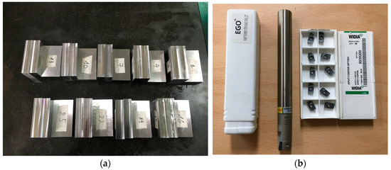
Figure 1.
(a) Test samples; (b) Tool holder and cutting inserts.
2.2. MQL, Machine Tool and Measuring Devices
The energy released in the main cutting region is inevitable. It is the result of molecular bonds being broken on the workpiece. Some heat is transferred to the workpiece and the rest to the chip. Friction generating heat between the chip and the tool in the secondary cutting zone causes the tool and the chip to heat up. In this area, heat significantly accelerates tool wear and considerably affects cutting force and surface roughness. The properly implemented MQL will greatly reduce this heat by lubricating the chip–cutting tool contact area. The lubrication system in this research is the minimum quantity lubrication system of TOPSET, Beijing, China. The system could install up to 2 nozzles, each 6 mm in diameter. In this investigation, peanut oil served as the lubricant.
This research was carried out on the 5-axis machining center DMG DMU 50. This machine tool is a small-sized machine suitable for research and training needs. The machine’s maximum spindle speed is 14,000 RPM, thus extending the input variable boundary condition to various experiments. The general structure of the experimental system is represented in Figure 2.
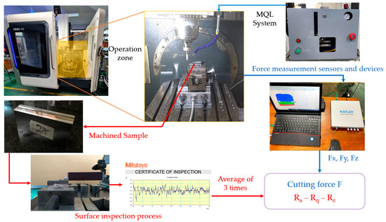
Figure 2.
Experimental system diagram.
The study team used force sensors from Kistler, Switzerland to build a force measurement system for the experiment. A Kistler 9139AA sensor with a possible measuring area from −30,000 N to 30,000 N, through the company’s self-developed specialized data collection software named DynoWare, gave assistance to store and inspect force data from 3 directions, corresponding to Fx, Fy, and Fz. Based on these results, the combined cutting force was calculated and examined.
The Portable Surface Tester SJ-210 from Mitutoyo is used to measure the surface roughness Ra. Meanwhile, the Surftest SJ-series USB Communication Version 5.007A application displays and records measurement parameters in various standards, but this work only considers the data in ISO 4287:1997. Three measurements were taken for each experiment. The empirical values were analyzed and evaluated using the average value of these.
2.3. Experimental Design
Five input parameters, including cutting velocity (Vc), tooth feed rate (fz), axial depth of cut (ap), MQL nozzle pressure (P), and MQL flow rate (Q) are surveyed to build the experiment matrix for this study. An experimental analysis and prediction of milling force and surface roughness were performed using three input levels in the Taguchi orthogonal model. As recommended by the cutting tool manufacturer, and the limit specifications of the machining center and lubrication system, the investigation parameters for hardened S50C steel should consider the ranges listed in Table 3.
Table 3.
Input parameters.
The parameters are selected and sorted according to the input parameter levels to implement Taguchi’s orthogonal experimental planning theory. These data are shown in Table 3. By surveying five input parameters at three different values, 27 experiments were designed based on the L27-35 experimental matrix in the Taguchi orthogonal array designs theory.
2.4. Research Methodology
2.4.1. Support Vector Regression
Machine learning classification problems are frequently and extensively solved using support vector machines (SVM). An SVM’s objective is to choose the best hyperplane (which can be either a plane or a curve) for dividing the data into two distinct areas, with the closest point to the hyperplane being as far away from it as possible. This is also known as the margin. The hyperplane and margin are depicted in Figure 3.
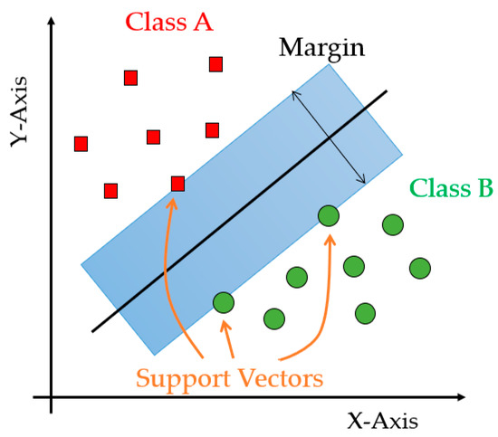
Figure 3.
Illustration of the hyperplane and the margin.
Take as the hyperplane’s equation. Finding and maximizing the margin is the objective of the SVM algorithm. The support vector machine (SVM) algorithm can also solve regression problems, commonly known as support vector regression (SVR). Contrary to the classification task, where the margin must be free of all data points, the margin now needs to cover all data points. In this instance, the regression model used to estimate the y values for given x values is represented by a geometrical boundary in the middle of the margin; on this premise, the boundary symbolizes the model function. Similar to classification, soft margins could also be used for the regression model, which allows a few investigated data points to be outside the margin.
The Vapnik loss function [30,31], describes how the SVR algorithm is error-tolerant for points within a small epsilon of the true value. This indicates that this function yields zero error for every training set point within the epsilon range. Figure 4a,b exhibit linear and non-linear regression in the epsilon range [31], respectively.
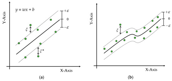
Figure 4.
(a) Linear regression with the epsilon range; (b) Non-linear regression with the epsilon range.
Support vector regression and simple linear regression seem similar; both have a linear assumption in mind. With hard margins, SVR is sensitive to outliers because the margin includes even the outliers; it is different than linear regression. To avoid that, soft margins are used to make SVR more similar to linear regression. In contrast to linear regression, SVR takes only the outermost data points into account but does not affect only outliers. Observing a group of data within the margin, SVR is less sensitive to this group than simple linear regression. Simple linear regression uses a cost function like mean squared error, which takes all data points into account, and a group of data points gives much more weight to the cost function, which attracts the model line. Generally, linear regression takes all data points into account, contrary to SVR. Nevertheless, support vector regression is an immensely efficient algorithm because it is determined by the support vectors covering the margin boundaries.
SVR has a very efficient option to incorporate non-linearity. The dual formulation of the cost function gives an appropriate way to solve variable transformations via the kernel trick and could also be transferred to SVR. With SVR and the kernel trick in the dual formulation, the problems with non-linear data distributions would be tackled.
2.4.2. Non-Dominated Sorting Genetic Algorithm II (NSGA-II)
Numerous new multi-objective optimization techniques have been introduced over the years to replace single-objective optimization GA. They include MOGA, NSGA-II, SPEA, Micro-GA, PAES, etc. [32,33,34,35]. Furthermore, NSGA-II has been proven highly effective for optimizing the machining process parameters of all MOGA techniques. One of the most well-known multi-objective optimization algorithms, NSGA-II, includes three distinctive features: a quick strategy for non-dominated sorting, a speedy approach for crowded distance estimation, and a swift mechanism for crowded comparison [35]. Mitra [36] optimized several test issues from earlier studies using the NSGA-II optimization method, which led to the conclusion that this was superior to PAES and SPEA when used to identify optimal solutions.
The general method of machining process parameter optimization using NSGA-II is shown in Figure 5. An analysis of experimental data is used to develop a model that correlates the input and output data in machining. Relationships between the machining performances and process parameters are typically generated using regression analysis, artificial neural networks (ANN), or fuzzy logic. The NSGA-II is designed as an optimization problem with the process parameters acting as decision variables in order to find the fitness values, which are minimized or maximized depending on the process parameters.
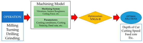
Figure 5.
The strategy for deploying the optimization problem in machining.
The NSGA-II can be broadly described as a series of steps:
- Step 1: Population initialization: Set up the population in accordance with the scope of the issue.
- Step 2: Non-dominated sort: Sorting is performed in accordance with the population’s non-domination principles.
- Step 3: Crowding distance: The front-wise crowding distance is computed following sorting. Individuals are chosen based on rankings and crowding distances.
- Step 4: Selection: The crowded-comparison approach is used to identify individuals in binary tournaments.
- Step 5: Genetic operators: Binary crossover and polynomial mutation are used in real-coded GA.
- Step 6: Recombination and selection: The chosen members of the following generation are identified once the current generation population and offspring population have been combined. As each front succeeds in filling the new generation, the population size increases until it surpasses the existing population.
This study delves into finding the optimization parameter set by using NSGA-II with the input parameter set obtained through processing by the regression application of the SVM algorithm. Figure 6 explains the implementation of the proposed multi-objective optimization of surface roughness and cutting force in the machining process.
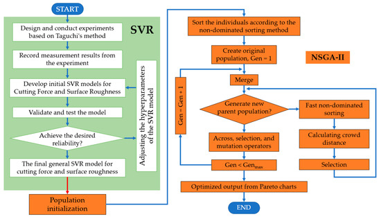
Figure 6.
Multi-objective optimization flow chart for surface roughness and cutting force in the milling process using SVR–NSGA-II combination.
3. Results and Discussion
3.1. Regression and Experimental Results
In our case, firstly, we used SVR to build a model for the surface roughness (Ra), the root mean square deviation of the profile (Rq), the average height difference between the highest peak and the lowest valley over five sampling lengths (Rz), and combined cutting force (F). Assuming that , , , and .
In order to build the linear model for SVR, which was based on the dimension feature space by Equation (1), the input x was first mapped into the m dimension feature space by a non-linear mapping function.
where with is a series of non-linear mapping functions.
The loss function L(y, f(x,w)) evaluates the estimate’s accuracy. Epsilon, an insensitive loss function proposed by Vapnik, is the loss function used by SVR [30,31]:
Therefore, SVM employs the function L to conduct linear regression in multi-dimension feature space and lowers model complexity by minimizing . By adding the slug variables, and , and setting i = 1, 2, … n to assess the deviation of the training samples that are outside the epsilon range, this issue can be resolved. As a result, SVR is minimized using the function:
with constrains:
The function f(x) is finally obtained by using the duality theorem for minimizing issues:
where n is the number of support vectors, and denotes the kernel function, which is defined as
Using the application of SVR, we developed models to forecast surface roughness (Ra) and cutting force (F) with C = 10 × 105 and ε = 0.01. The performance of the model is presented in Table 4.
Table 4.
Experimental result and performance of SVR models.
We proceeded to build the predictive regression line of the model using both the experimental matrix and experimental results. The regression line that best fits the desired data is obtained after repeated attempts at adjusting the hyperparameters of the SVR model. Figure 7a,b illustrate the SVR predictions for Ra, Rq, Rz, and F compared to the expected output.
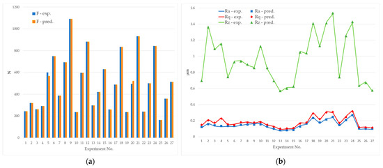
Figure 7.
SVR prediction output and experimental results: (a) Cutting Force; (b) Ra–Rq–Rz.
As depicted in Figure 7, the predicted values derived from the SVR and the measured values obtained from the experiment are remarkably comparable, including the overall pattern. Observing the shear force results reveals that Experiment 5 and Experiment 20 have the greatest variance, at 5.59 and 5.40 percent, respectively. The deviation values generally fall within the acceptable range, and the predicted results are reasonable. Regression results obtained from the SVR method have the model’s goodness of fit (R-score) calculated as in Equation (7). The R-score for the surface evaluation criteria such as Ra, Rq, Rz, and cutting force regression models were calculated with highly positive outcomes, at 97.3%, 98.82%, 99.9%, and 99.9%, respectively.
The R-score ranges from 0 to 1, with a higher value indicating a better fit between the SVR model and the experimental data. A value of 0 indicates that the model explains no variance in the target variable, whereas a value of 1 indicates that the model perfectly explains all variance in the target variable.
3.2. Multi-Objective Optimization
Multi-objective optimization optimizes various objective functions subject to inequality and equality constraints [37]. It is desirable to find solutions that violate no constraints and are as good as possible concerning all objectives. Therefore, a set of trade-off solutions between many objectives results from such a multi-objective optimization problem. These trade-off points are known as Pareto optimum solutions because they can only be improved in the case of at least one other objective, thereby making matters worse as they are not dominated by any other solution. The Pareto optimal solution set and all of these possible non-dominated alternatives are collectively referred to as the Pareto front [38]. Following the termination of the optimization process, the final population will contain non-dominated solutions that are Pareto-optimal with a reasonable degree of variety.
The similarity in the tendency of Ra, Rq, and Rz during the experiment was obviously shown in Figure 7. Therefore, to reduce the complication of the model, the authors implement optimization only with the surface roughness parameter Ra and the cutting force F.
From the obtained regression results, we use a non-dominated sorting genetic algorithm (NSGA-II) to perform multi-object optimization. In this case, we need to minimize and . Python Sklearn and Pymoo frameworks are used to implement SVR and multi-object optimization. The optimal results of the NSGA-II for a population size of 50 and 1000 generations are shown in Table 5.
Table 5.
The calculated optimal set.
In Figure 8, the Pareto for the optimization of two objectives of and is graphically represented. Both and are approximated by the SVR model. This graph illustrates a set of trade-off solutions between Ra and F objective functions. These optimal solutions at trade-off points are non-dominated and cannot be improved with regard to at least one objective without causing a decline in performance. The study obtained the optimal parameters of roughness and cutting force as Ra = 0.050 µm, F = 226.691 N with P = 3.945 MPa, Q = 123.247 mL/h, Vc = 195.193 m/min, fz = 0.020 mm/tooth, and ap = 0.100 mm when giving priority to surface roughness Ra. When the focus is on the cutting force, the optimal set of parameters is P = 5.997 MPa, Q = 59.461 mL/h, Vc = 185.782 m/min, fz = 0.020 mm/tooth, and ap = 0.100 mm, resulting in the surface roughness Ra = 0.094 µm and the cutting force F = 126.611 N. When both output parameters Ra and F are held at their neutral values, Ra = 0.066 µm and F = 167.126 N, the optimum parameters are P = 5.503 MPa, Q = 115.504 mL/h, Vc = 188.186 m/min, fz = 0.020 mm/tooth, and ap = 0.100 mm.
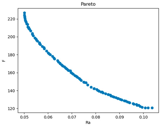
Figure 8.
The Pareto for the optimization of two objectives of Ra and F.
3.3. Discussion
This study presented a regression method with SVR combined with multi-objective optimization with the NSGA-II algorithm. With this approach, it obviously shows that reliability is superior to other conventional methods, especially in regression results. The response surface method (RSM), one of the statistical analysis methods, was applied to analyze the experimental data set which was presented in this paper [26]. The regression results obtained from the RSM method are fairly favorable if the study only focused on the fitness of the model compared with the experimental data, but when more concerned about the predictability, this model was not comprehensive. According to the previous calculation, the predicted root mean square (R-sq (pred)) for surface roughness and cutting force regression results of RSM were 59.06% and 85.35%, respectively [26]. This suggests that model overfitting or underfitting occurs when adding terms for effects that are not important in the population. Therefore, prediction based on the whole population may not be useful when the model is fit to a sample data set. This problem has been completely solved when using the model proposed in this study, with the advantage of SVR to avoid the issues of underfitting and overfitting, along with the reliability of up to 97.30% for the surface roughness model and 99.90% for the cutting force model.
Validation experiments were carried out to verify the proposed optimal set of parameters. Due to the restriction in controlling the flow rate of the minimum lubrication system, the two control levels that fitted to the proposed parameter set were selected. Figure 9 depicts the surface machined with the suggested set of optimal conditions. The results of the verification experiments, as shown in Table 6, express that the deviation from the optimal results obtained from NSGA-II is within a permissible range, with 8.94% for surface roughness and 3.21% for cutting forces results.
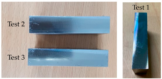
Figure 9.
Machined surfaces of the validation experiment.
Table 6.
Validation experiment for neutral priority optimization.
4. Conclusions
An approach combining NSGA-II and SVR to investigate the milling process of S50C carbon steel has been proposed in an effort to optimize surface roughness and cutting force. To predict and optimize the surface quality and cutting force, variables from the cutting parameters Vc, fz, and ap, as well as factors from the MQL system, P and Q, were considered. The parameters are optimized through the NSGA-II algorithm, with the model’s input data being processed through the SVR technique. As a result, we derive the following conclusions:
- The study has succeeded in proposing a plan to improve the reliability in building the regression model compared to previous studies by applying the SVR technique to obtain regression results for the model. The reliability of the regression model using the SVR algorithm is remarkably high, reaching 97.30% and 99.80% for the surface roughness and cutting force regression models, respectively.
- A hybrid method based on SVR and NSGA-II has proven reliable and could be applied in manufacturing to determine the optimal parameters. As a result of combining the SVR and NSGA-II methods in this study, an optimal set of parameters, which included Ra = 0.066 µm and F = 126.611 N, along with P = 5.503 MPa, Q = 115.504 mL/h, Vc = 188.186 m/min, fz = 0.020 mm/tooth, and ap = 0.100 mm, was suggested.
- The insignificant disparity between the results of the validation experiments and the suggested parameters demonstrates the viability and accuracy of the research. Nonetheless, it was evident that some parameters of the optimal set will inevitably fall outside the system’s control levels, making it challenging to apply the optimized cutting conditions in machining.
- The study made notable contributions to the reference data of S50C steel after heat treatment, which was known as a high-hardness material.
Author Contributions
T.-C.N. designed and conducted experiments, synthesized data, and wrote the original manuscript; Q.-C.H. supervised, reviewed, and edited the content; D.H.T., instructed, and edited the manuscript; B.-N.N. analyzed the results and reviewed the manuscript. All authors have read and agreed to the published version of the manuscript.
Funding
This research received no external funding.
Acknowledgments
The authors would like to thank the Faculty of Mechanical Engineering, Hanoi University of Industry, Hanoi, Vietnam for creating favorable conditions to use the equipment and workshops as well as for valuable help and discussion in this research process.
Conflicts of Interest
The authors declare no conflict of interest.
References
- Richt, C. Hard turn toward efficiency. Gear Solutions, 1 April 2009, pp. 22–30. Available online: https://gearsolutions.com/features/a-hard-turn-toward-efficiency/ (accessed on 16 April 2023).
- Nguyen, T.; Hoang, T.D.; Dao, N.H.; Do Minh, H. The prediction and optimization of surface roughness in grinding of S50C carbon steel using minimum quantity lubrication of vietnamese peanut oil. J. Appl. Eng. Sci. 2021, 19, 814–821. [Google Scholar]
- Abdullah, B.; Nordin, M.F.M.; Basir, M.H.M. Investigation on CR, MRR and SR of wire electrical discharge machining (WEDM) on high carbon steel S50C. J. Teknol. 2015, 76, 109–113. [Google Scholar] [CrossRef]
- Masmiati, N.; Sarhan, A.A.; Hassan, M.A.N.; Hamdi, M. Optimization of cutting conditions for minimum residual stress, cutting force and surface roughness in end milling of S50C medium carbon steel. Measurement 2016, 86, 253–265. [Google Scholar] [CrossRef]
- Dubey, V.; Sharma, A.K.; Vats, P.; Pimenov, D.Y.; Giasin, K.; Chuchala, D. Study of a multicriterion decision-making approach to the MQL turning of AISI 304 steel using hybrid nanocutting fluid. Materials 2021, 14, 7207. [Google Scholar] [CrossRef]
- Qazi, M.I.; Abas, M.; Khan, R.; Saleem, W.; Pruncu, C.I.; Omair, M. Experimental investigation and multi-response optimization of machinability of AA5005H34 using composite desirability coupled with PCA. Metals 2021, 11, 235. [Google Scholar] [CrossRef]
- Salur, E.; Kuntoğlu, M.; Aslan, A.; Pimenov, D.Y. The effects of MQL and dry environments on tool wear, cutting temperature, and power consumption during end milling of AISI 1040 steel. Metals 2021, 11, 1674. [Google Scholar] [CrossRef]
- Kang, M.; Kim, K.; Shin, S.; Jang, S.; Park, J.; Kim, C. Effect of the minimum quantity lubrication in high-speed end-milling of AISI D2 cold-worked die steel (62 HRC) by coated carbide tools. Surf. Coat. Technol. 2008, 202, 5621–5624. [Google Scholar] [CrossRef]
- Mia, M.; Al Bashir, M.; Khan, M.A.; Dhar, N.R. Optimization of MQL flow rate for minimum cutting force and surface roughness in end milling of hardened steel (HRC 40). Int. J. Adv. Manuf. Technol. 2017, 89, 675–690. [Google Scholar] [CrossRef]
- Mirjalili, S. Genetic algorithm. In Evolutionary Algorithms and Neural Networks; Springer: Cham, Switzerland, 2019; pp. 43–55. [Google Scholar]
- Mahesh, G.; Muthu, S.; Devadasan, S. Prediction of surface roughness of end milling operation using genetic algorithm. Int. J. Adv. Manuf. Technol. 2015, 77, 369–381. [Google Scholar] [CrossRef]
- Li, J.; Yang, X.; Ren, C.; Chen, G.; Wang, Y. Multiobjective optimization of cutting parameters in Ti-6Al-4V milling process using nondominated sorting genetic algorithm-II. Int. J. Adv. Manuf. Technol. 2015, 76, 941–953. [Google Scholar] [CrossRef]
- Selvam, M.D.; Dawood, D.; Karuppusami, D.G. Optimization of machining parameters for face milling operation in a vertical CNC milling machine using genetic algorithm. IRACST-Eng. Sci. Technol. Int. J. 2012, 2, 544–548. [Google Scholar]
- Abu-Mahfouz, I.; Banerjee, A.; Rahman, E. Evolutionary optimization of machining parameters based on surface roughness in end milling of hot rolled steel. Materials 2021, 14, 5494. [Google Scholar] [CrossRef]
- Sangwan, K.S.; Kant, G. Optimization of machining parameters for improving energy efficiency using integrated response surface methodology and genetic algorithm approach. Procedia CIRP 2017, 61, 517–522. [Google Scholar] [CrossRef]
- Sangwan, K.S.; Saxena, S.; Kant, G. Optimization of machining parameters to minimize surface roughness using integrated ANN-GA approach. Procedia CIRP 2015, 29, 305–310. [Google Scholar] [CrossRef]
- Kilickap, E.; Huseyinoglu, M.; Yardimeden, A. Optimization of drilling parameters on surface roughness in drilling of AISI 1045 using response surface methodology and genetic algorithm. Int. J. Adv. Manuf. Technol. 2011, 52, 79–88. [Google Scholar] [CrossRef]
- Kuruvila, N. Parametric influence and optimization of wire EDM of hot die steel. Mach. Sci. Technol. 2011, 15, 47–75. [Google Scholar] [CrossRef]
- Pasam, V.K.; Battula, S.B.; Madar Valli, P.; Swapna, M. Optimizing surface finish in WEDM using the Taguchi parameter design method. J. Braz. Soc. Mech. Sci. Eng. 2010, 32, 107–113. [Google Scholar] [CrossRef]
- Zolpakar, N.A.; Lodhi, S.S.; Pathak, S.; Sharma, M.A. Application of multi-objective genetic algorithm (MOGA) optimization in machining processes. In Optimization of Manufacturing Processes; Springer: Cham, Switzerland, 2020; pp. 185–199. [Google Scholar]
- Cho, S.; Asfour, S.; Onar, A.; Kaundinya, N. Tool breakage detection using support vector machine learning in a milling process. Int. J. Mach. Tools Manuf. 2005, 45, 241–249. [Google Scholar] [CrossRef]
- Kadirgama, K.; Noor, M.; Rahman, M. Optimization of surface roughness in end milling using potential support vector machine. Arab. J. Sci. Eng. 2012, 37, 2269–2275. [Google Scholar] [CrossRef]
- Deris, A.M.; Zain, A.M.; Sallehuddin, R. Overview of support vector machine in modeling machining performances. Procedia Eng. 2011, 24, 308–312. [Google Scholar] [CrossRef]
- Samadzadegan, F.; Soleymani, A.; Abbaspour, R.A. Evaluation of genetic algorithms for tuning SVM parameters in multi-class problems. In Proceedings of the 2010 11th International Symposium on Computational Intelligence and Informatics (CINTI), Budapest, Hungary, 18–20 November 2010; pp. 323–328. [Google Scholar]
- Chunhong, Z.; Licheng, J. Automatic parameters selection for SVM based on GA. In Proceedings of the Fifth World Congress on Intelligent Control and Automation (IEEE Cat. No. 04EX788), Hangzhou, China, 15–19 June 2004; pp. 1869–1872. [Google Scholar]
- Nguyen, T.C.; Pham, T.T.T.; Dung, H.T. Research of multi-response optimization of milling process of hardened S50C steel using minimum quantity lubrication of Vietnamese peanut oil. EUREKA Phys. Eng. 2021, 6, 74–88. [Google Scholar]
- Do, T.-V.; Hsu, Q.-C. Optimization of minimum quantity lubricant conditions and cutting parameters in hard milling of AISI H13 steel. Appl. Sci. 2016, 6, 83. [Google Scholar] [CrossRef]
- Alsoruji, G.S.; Sadoun, A.; Abd Elaziz, M.; Al-Betar, M.A.; Abdallah, A.; Fathy, A. On the prediction of the mechanical properties of ultrafine grain Al-TiO2 nanocomposites using a modified long-short term memory model with beluga whale optimizer. J. Mater. Res. Technol. 2023, 23, 4075–4088. [Google Scholar] [CrossRef]
- Najjar, I.R.; Sadoun, A.M.; Fathy, A.; Abdallah, A.W.; Elaziz, M.A.; Elmahdy, M. Prediction of Tribological Properties of Alumina-Coated, Silver-Reinforced Copper Nanocomposites Using Long Short-Term Model Combined with Golden Jackal Optimization. Lubricants 2022, 10, 277. [Google Scholar] [CrossRef]
- Vapnik, V. The Nature of Statistical Learning Theory; Springer Science & Business Media: New York, NY, USA, 1999. [Google Scholar]
- Vapnik, V.N. Statistical Learning Theory; Adaptive and Learning Systems for Signal Processing, Communications and Control; Wiley: Hoboken, NJ, USA, 1998; Volume 2, pp. 1–740. [Google Scholar]
- Datta, R.; Deb, K. A classical-cum-evolutionary multi-objective optimization for optimal machining parameters. In Proceedings of the 2009 World Congress on Nature & Biologically Inspired Computing (NaBIC), Coimbatore, India, 9–11 December 2009; pp. 607–612. [Google Scholar]
- Chen, J. Multi-objective optimization of cutting parameters with improved NSGA-II. In Proceedings of the 2009 International Conference on Management and Service Science, Beijing, China, 20–22 September 2009; pp. 1–4. [Google Scholar]
- Kodali, S.P.; Kudikala, R.; Kalyanmoy, D. Multi-objective optimization of surface grinding process using NSGA II. In Proceedings of the 2008 First International Conference on Emerging Trends in Engineering and Technology, Nagpur, India, 16–18 July 2008; pp. 763–767. [Google Scholar]
- Deb, K.; Pratap, A.; Agarwal, S.; Meyarivan, T. A fast and elitist multiobjective genetic algorithm: NSGA-II. IEEE Trans. Evol. Comput. 2002, 6, 182–197. [Google Scholar] [CrossRef]
- Mitra, K. Multiobjective optimization of an industrial grinding operation under uncertainty. Chem. Eng. Sci. 2009, 64, 5043–5056. [Google Scholar] [CrossRef]
- Deb, K. Multi-Objective Optimisation Using Evolutionary Algorithms: An Introduction; Springer: London, UK, 2011. [Google Scholar]
- Konak, A.; Coit, D.W.; Smith, A.E. Multi-objective optimization using genetic algorithms: A tutorial. Reliab. Eng. Syst. Saf. 2006, 91, 992–1007. [Google Scholar] [CrossRef]


Disclaimer/Publisher’s Note: The statements, opinions and data contained in all publications are solely those of the individual author(s) and contributor(s) and not of MDPI and/or the editor(s). MDPI and/or the editor(s) disclaim responsibility for any injury to people or property resulting from any ideas, methods, instructions or products referred to in the content. |
© 2023 by the authors. Licensee MDPI, Basel, Switzerland. This article is an open access article distributed under the terms and conditions of the Creative Commons Attribution (CC BY) license (https://creativecommons.org/licenses/by/4.0/).