Abstract
In this work, the dry turning of Inconel 601 alloy in a dry environment with PVD-coated cutting inserts was studied. Turning was performed at various cutting speeds, feeds, insert shapes, corner radii, rake angles, and approach angles. After machining, arithmetic mean surface roughness (Ra) and flank wear (VB) were measured, and the material removal rate was also calculated (MRR). An analysis of variance (ANOVA) was performed to determine the effects of the turning input parameters. For the measured values, the turning process was modeled using an artificial neural network (ANN). Based on the obtained model, the process parameters were optimized using a genetic algorithm (GA). The objective function was to simultaneously minimize Ra and VB and maximize MRR. The accuracy of the model and the optimal values were further validated by confirmation experiments. The maximum percentage errors, which are less than 2%, indicate the possibility of practical implementation of the hybrid approach for modeling and optimization of dry turning of Inconel 601 alloy.
1. Introduction
Inconel alloys are a difficult-to-cut material and are therefore characterized by poor machinability. For this reason, Inconel is usually machined wet or near-dry. However, dry turning is the least harmful to the environment, and the shavings are the easiest to recycle. In addition, costs are lower with dry turning because there are no costs for lubricants, additional equipment, collection, treatment, etc. The main problem with dry turning is the occurrence of higher temperatures and more intensive tool wear. This can result in poor surface quality, out-of-tolerance manufacturing, poor geometric product specification, etc. In order to achieve acceptable surface roughness, longer tool life, and required productivity in dry turning, a large number of parameters, such as tool material, tool coating, tool geometry, cutting speed, feed, depth of cut, etc., must be controlled and optimized. [1,2,3].
The dry turning of Inconel alloys has been investigated in numerous theoretical, simulation, and experimental studies from various aspects. Li et al. [4] experimented with different inserts. The results show that PVD-coated inserts are more suitable for turning than CVD-coated cutting inserts. Ceramic cutting inserts with a negative rake angle and round shape gave the best results. Devillez et al. [5] evaluated the performance of multilayer and nanostructured TiAlN and AlTiN coatings on cemented carbide tools. The dominant wear modes observed during dry cutting were welding and adhesion of workpiece material to the rake and flank surfaces. Nalbant et al. [6] investigated the effects of cutting tool material and cutting speed on cutting forces and tool wear. Plastic deformation, flank wear, and notch wear and build-up at high cutting speeds were determined. Outeiro et al. [7] studied the residual stresses induced by dry turning with coated and uncoated cemented carbide tools. Machining with the uncoated tool produced higher surface residual stresses than with the coated tool. The higher residual stress values were obtained on the transient surface rather than the machined surface. Attia et al. [8] established the optimum conditions for laser-assisted dry turning with ceramic tools. The surface roughness and the MRR were improved while cutting forces were reduced. Akhyar Ibrahim et al. [9] investigated the wear mechanisms of TiAIN carbide cutting inserts at different cutting speeds, depths of cut, and feeds using the Taguchi method. The wear mechanism types were abrasive wear on the flank and rake surface and cracks and fractures on the cutting edge. The most significant factor affecting wear was the depth of cut, followed by feed and cutting speed. Umbrello [10] investigated the effects of cutting conditions on surface roughness and hardness. Higher cutting speeds and feeds allow the material to have a higher surface hardness and a deeper hardness variation. Ramanujam et al. [11] used the Taguchi method to optimize dry turning parameters to evaluate the performance parameters such as cutting force, surface roughness, and tool wear. The results showed that feed and depth of cut had the greatest influence on the responses. Ramanujam et al. [12] used the fuzzy method with the Taguchi method to optimize machining parameters for minimum surface roughness and power consumption and maximum MRR. It was found that feed is the most important factor contributing to most of the variations. Satyanarayana et al. [13] used GA to predict the optimum values for cutting speed, depth of cut, and feed considering MRR and surface roughness. Thakur et al. [14] investigated the effects of cutting speed on chip morphology, chip thickness ratio, tool wear, and surface integrity for uncoated and coated tools. The positive effect of coated tools over uncoated was most evident when machining at high cutting speeds. Thakur and Gangopadhyay [15] evaluated cutting force, cutting temperature, tool wear, and surface integrity. The results obtained in both roughing and finishing operations support the use of PVD-coated tools in dry, dry environments. Vetri Velmurgan and Venkatesan [16] investigated the effect of cutting speed, feed, and depth of cut on cutting force and surface roughness based on the Taguchi method. The most significant factor in the cutting force and roughness was the depth of the cut. Liu et al. [17] investigated the cutting performance and wear mechanism after the deposition of the TiCN coating on the surface of Sialon ceramic cutting inserts. The tool life of the TiCN-coated cutting inserts was significantly longer than that of the uncoated ones. Zeilmann et al. [18] evaluated the performance of various conditions during turning with ceramic tools. The predominant wears were notch wear and flank wear. Thakur and Gangopadhyay [19] studied the effect of cutting speed and tool coating on chip morphology, shear band thickness, equivalent chip thickness, and different features of segmented chips. The results showed that the coated tool restricted a sharp increase in shear band thickness with cutting speed and resulted in a reduction in tooth distance, tooth angle, equivalent chip thickness, chip hardness, and deformation on grains while exhibiting an increase in chip segmentation frequency in comparison with the uncoated tool. Cantero et al. [20] compared several PCBN tools with a reference carbide insert in wet and dry environments. PCBN inserts showed reasonable MRR and surface quality. Additionally, the results showed that the high-speed turning of Inconel was not suitable in a dry environment. Hua and Liu [21] investigated the effects of cutting speed, feed, and corner radius on surface roughness and degree of work hardening. The results indicate that the feed and corner radius has a dominant effect on the surface roughness. The results also show that the degree of work hardening increased with increasing cutting speed and feed. Qiu et al. [22] investigated the influence of J-C constitutive model parameters and friction coefficient on residual stress, chip morphology, cutting force, and temperature. The results demonstrated that the simulation accuracy was more susceptible to strain hardening and thermal softening in the J-C constitutive model. The friction coefficient had significant effects on the cutting forces. Hemakumar and Kuppan [23] investigated the effect of cutting speed and feed on cutting force, surface roughness, and flank wear. Empirical models were developed using response surface methodology (RSM). Feed was the most influencing parameter for cutting force and surface roughness while cutting speed was the most influencing parameter for flank wear. Shalaby Veldhuis [24] investigated tool wear and chip formation with different ceramic tools. The results showed that alumina with added ZrO2 had the best resistance to abrasive wear. It was found that the chipping and notching of the tool decreased with increasing cutting speed. Qadria et al. [25] assessed the effect of workpiece hardness at different cutting speeds on tool tip temperature and tool life with different ceramic tools. The Al-oxide cutting insert had better cutting performance and lower crater wear. Zhao and Liu [26] investigated PVD TiAlN tools with different coating thicknesses. The results showed that tools with lower coating thickness had better friction effects and lower cutting temperatures. Peng et al. [27] presented a semi-empirical approach to predict the residual stress. The distributions of the predicted residual stress and the experimental data showed the hook shape. Vukelic et al. [28] presented a methodology to evaluate the dry-turning process along with optimum machining parameters. Acceptable flank wear and required surface quality, while reducing cutting time and energy consumption, were achieved with larger corner radii and cutting speeds and smaller feeds and depths of cut. Ren et al. [29] analyzed the effect of turning process parameters on surface integrity and fatigue life. The results indicated that the degree of work hardening, residual stress in the cutting speed direction, fatigue stress concentration factor, degree of grain refinement, and residual stress in the feed direction are the most important influencing parameters. Veerappan et al. [30] investigated surface roughness and tool wear. The greatest influence on surface roughness and tool wear had cutting speed, followed by feed and depth of cut. Yashwant Bhise and Jogi [31] studied the influence of cutting speed and feed on surface roughness. The feed had a greater impact on surface roughness. Zhao et al. [32] analyzed the effects of Al content on TiAlN coating properties. Anti-friction, thermal barrier, and tool life improve with increasing Al content. Xue et al. [33] investigated the wear mechanisms of SiC whisker-reinforced alumina and Sialon. The results showed that the wear process of SiC whisker-reinforced alumina was dominated by notch wear, while flank wear, characterized by ridges and grooves, was the main wear mode for Sialon. Szablewski et al. [34] proposed a new cutting insert that produced similar surface roughness to wiper inserts. The lowest surface roughness values were obtained at the lowest feed. Sticking was dependent on feed and cutting-edge effective length. Grigoriev et al. [35] studied the tribological properties of coatings and wear resistance. A coating with active oxidation exhibits better wear resistance than a slightly oxidized coating. Dhananchezian [36] investigated the effect of cutting speed on surface roughness. With increasing cutting speed, the surface roughness decreases.
All previous approaches to the study of dry turning of Inconel alloys have their advantages and disadvantages. Most of these studies have examined the effects of machining parameters, i.e., cutting speed, feed, and depth of cut, on the performance characteristics of the turning process. The most commonly studied process performance was machined surface roughness, tool life, machining time, etc. The disadvantage of experimental research, especially under the conditions of a large number of experiments, is that it is expensive and time-consuming. In order to overcome these disadvantages, suitable models are developed in the research. Modeling the relationship between input–output parameters involves cause–effect relationships. Theoretical modeling is based on process physics and physical phenomena. The main difficulty in developing these methods is that a thorough knowledge of the process is required, which is not always possible given the limited availability of information. An alternative modeling approach is empirical modeling. Empirical modeling methods are based on experimental data, i.e., finding a functional dependence between the input and output parameters of the process. Empirical modeling techniques such as the Taguchi method, ANN, fuzzy logic, RSM, and SVM are most commonly used for modeling the turning process. The basic problems to be solved are economical and efficient data collection, filtering noisy data (outliers), and defining the statistical characteristics of the data. It is critical that the errors between the predicted and experimental values be within acceptable limits so that the predictive model can be used in practice. As accuracy increases, the established relationships should converge. When the process is modeled correctly, the subjective influence of the operator on the results obtained is also reduced. Additionally, the universality and, thus, the possibility of practical application are greater since the models can be applied in the range of input parameters and not only for experimental data. The main problem is the question of which method to use and when since each method has its own advantages and disadvantages. Notwithstanding some existing guidelines, it is still impossible to define an algorithm for selecting an appropriate method. Additionally, the development of predictive models is the basis for process optimization on various grounds. Global evolutionary optimization techniques, such as GA, PSO, etc., are most commonly used to optimize the turning process. Each of the mentioned optimization methods has its advantages and disadvantages. Therefore, the crucial question is how to select an appropriate method, i.e., how to formulate a sufficiently accurate optimization model that represents a sufficiently accurate approximation of the process. Optimal combinations of input parameters depend on many factors since the turning process is characterized by many dynamic parameters. The individual input parameters can have both positive and negative effects on the various process outputs. At the same time, the magnitude of the positive or negative effect varies. Given the different and often conflicting requirements, it is necessary to perform multi-criteria optimization to find a compromise solution for the given production conditions.
The application of modeling and optimization methods is essential to minimize costs and maximize quality and productivity. Therefore, it is important to choose an appropriate method for modeling and optimization and to formulate a sufficiently accurate model. In contrast to the previous studies, the objective of this research is to evaluate, model, and optimize the influence of cutting insert geometry and turning process parameters of the Inconel 601 alloy, which have not been extensively studied in the literature so far. In this study, the influence of six input parameters (cutting speed, feed, insert shape, corner radius, rake angle, and approach angle) on three output parameters (surface roughness, flank wear, and material removal rate) was studied. The idea is to generate optimal combinations of input process parameters for different requirements of output process parameters. This means that for different levels of importance of quality, tool life, and productivity, different optimal combinations of input parameters of the process are obtained. Respecting the principles of environmental protection and occupational safety, the research was carried out as dry turning. With the development of a sufficiently accurate empirical model, the difficulties of production planning, selection of machining parameters, and cutting tools will be significantly reduced. In addition to modeling and optimization, a predictive model should also ensure the selection of adequate input parameters, i.e., their combination, based on which a compromise solution will be obtained after turning from the point of view of the roughness of the machined surface, tool life, and productivity.
2. Materials and Methods
The methodology by which the study was conducted is shown in Figure 1.
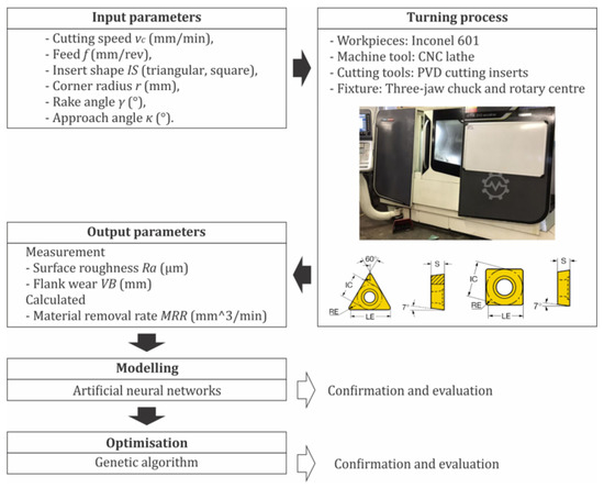
Figure 1.
The research methodology.
The research was conducted on workpieces made of Inconel 601 alloy, the chemical composition of which is as follows: (58–63)% nickel, (21–25)% chromium, (1–1.70)% aluminum, ≤1% copper, ≤1% manganese, ≤0.50% silicon, ≤0.10% carbon, ≤0.015% sulfur, and balanced % iron. The properties of Inconel 601 alloy are: density = 8.11 g/cm3, melting point = 1349 °C, tensile strength = 760 MPa, yield strength = 450 MPa, hardness = 160 HB, thermal expansion coefficient = 13.75 μm/m °C, and thermal conductivity = 11.2 W/mK. The dimensions of the workpieces are Ø 40 × 400 mm.
Dry turning is performed on the Mori Seiki CTX 310 Ecoline CNC lathe. Locating and clamping of the workpiece is carried out using a three-jaw chuck and rotary center. The characteristics of the cutting inserts are listed in Table 1.

Table 1.
The cutting inserts characteristics.
The experimental research was conducted according to the full factorial experiment. Six parameters were varied during the experimental study, namely: cutting speed, feed, insert shape, corner radius, rake angle, and approach angle. Following the manufacturer of the cutting inserts, the following input parameters were selected:
- Two levels for the cutting speed vc = 40/60 (mm/min);
- Two levels for the feed f = 0.15/0.25 (mm/rev);
- Two levels for the insert shape IS = triangular (T)/square (S);
- Three levels for the corner radius r = 0.4/0.8/1.2 (mm);
- Three levels for the rake angle γ = 3/6/9 (°);
- Three levels for the approach angle κ = 60/75/90 (°).
The arithmetic mean surface roughness and flank wear were measured after the experimental research, while the material removal rate (MRR) was calculated as MRR = vc·f·ap. The depth of cut (ap) was constant during the experimental investigation and was 1.5 mm.
Arithmetic mean surface roughness was measured using a Talysurf device (Figure 2a) with a stylus tip of 2 μm. Measurement of flank wear was performed using an optical microscope—LEITZ Orthoplan (Figure 2b)—with a 50× magnification and the ImageJ software package (version number 1.52 P).
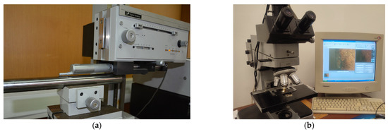
Figure 2.
Measurement process (a) arithmetic mean surface roughness; (b) flank wear.
After the measurements and calculations, the turning process is modeled and optimized. The process modeling was performed with an artificial neural network, while the optimization was performed with a genetic algorithm. Modeling and optimization performances were evaluated by calculating the percentage errors and by additional confirmation experiments.
3. Results
Since the experimental investigation was conducted in the form of a full factorial experiment, a total of 216 experiments were performed. The results of the measurements and calculations are shown in Table 2.
Table 2.
Results.
The experimental results were analyzed using Design Expert software. The classical sum of squares ANOVA was used to analyze the effects. Feed and cutting speed were treated as continuous factors, and insert shape, corner radius, rake angle, and approach angle as categorical factors. The graphical representation of the obtained results can be seen in Figure 3 and Figure 4.
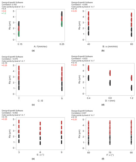
Figure 3.
Dependence of arithmetic mean surface roughness on input parameters (a) feed, (b) cutting speed, (c) insert shape, (d) corner radius, (e) rake angle, and (f) approach angle.
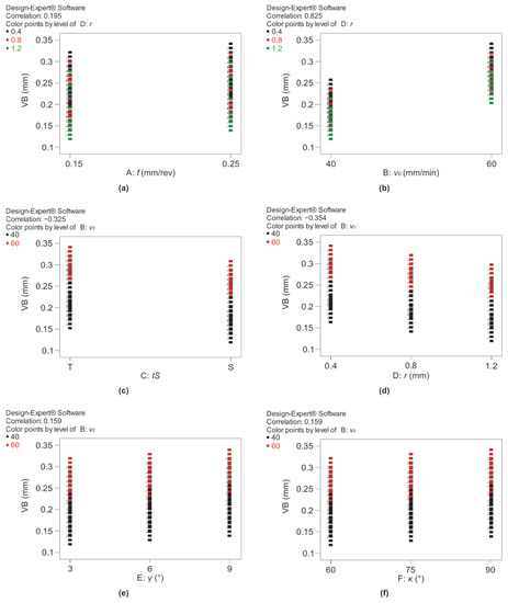
Figure 4.
Dependence of flank wear on input parameters (a) feed, (b) cutting speed, (c) insert shape, (d) corner radius, (e) rake angle, and (f) approach angle.
Figure 3 shows the dependence of arithmetic mean surface roughness on input parameters. The most influential parameters on the arithmetic mean surface roughness are feed (correlation coefficient 0.762) and corner radius (correlation coefficient −0.622), followed by cutting speed (correlation coefficient −0.095), insert shape (correlation coefficient 0.076), rake angle (correlation coefficient −0.062), and approach angle (correlation coefficient 0.047).
Table 3 shows the analysis of variance for the selected reduced regression model. The F value of the model 372.0577 means that the model is significant. The p-values less than 0.0500 indicate that the model factors of the model are significant, and in this case, A (feed), D (corner radius), and F (approach angle) are significant model factors.
Table 3.
ANOVA for arithmetic mean surface roughness.
Table 4 shows the summary indicators of the selected arithmetic mean surface roughness model. The coefficients of determination (original, adjusted, and for prediction) are 0.9696, 0.967, and 0.9639, respectively, and are not significantly different. The R2 value of 0.9696 means that approximately 97% of the variability in roughness is explained by feed, corner radius, and approach angle.
Table 4.
Summary indicators of the arithmetic mean surface roughness model.
The prediction equation for coded factors is:
Ra = 2.73437 + 0.85937·A + 0.859324·D [1] + 4.63 × 10⁻⁵·D[2] − 0.06444·F[1] + 1.85 × 10⁻⁵·F[2] + 1.85 × 10⁻⁵·A·D[1] + 4.63 × 10⁻⁵·A·D[2] − 2.3 × 10⁻⁵·A·F[1] + 1.85 × 10⁻⁵·A·F[2] − 8.8 × 10⁻⁵ · D[1]·F[1] + 2.31 × 10⁻⁵·D[2]·F[1] + 0.000162·D[1]·F[2] − 0.00014·D[2]·F[2] − 3.2 × 10⁻⁵·A·D[1]·F[1] + 0.000106·A·D[2]·F[1] − 3.24 × 10⁻⁵·A·D[1]·F[2] − 0.00014·A·D[2]·F[2]
Figure 4 shows the dependence of flank wear on input parameters. The most influential parameters on flank wear are cutting speed (correlation coefficient 0.825), corner radius (correlation coefficient −0.354), and insert shape (correlation coefficient 0.325), followed by feed (correlation coefficient 0.195), rake angle (coefficient correlation 0.159), and approach angle (correlation coefficient 0.159).
Flank wear decreases with decreasing feed (f), approach angle (κ), rake angle (γ), and cutting speed (v), and with increasing corner radius (r). Additionally, flank wear is lower for the S insert shape (IS).
Table 5 shows the analysis of variance for the selected reduced regression model. The F value of the model 305.88 means that the model is significant. The p-values less than 0.0500 indicate that the model factors are significant, and in this case, B (cutting speed), C (insert shape), and D (corner radius) are significant model factors.
Table 5.
ANOVA for flank wear.
Table 6 shows the summary indicators of the selected flank wear model. The adjusted coefficient of determination of 0.9085 is in agreement with the coefficient of determination for prediction of 0.9045.
Table 6.
Summary indicators of the flank wear model.
The prediction equation for coded factors is:
VB = 0.23 + 0.042·B − 0.017·C + 0.022·D[1] + 9.26 × 10⁻³·D[2] + 4.63 × 10⁻³·B·C − 7.87 × 10⁻²·B·D[1] + 1.57 × 10⁻¹·B·D[2]
A check of the adequacy of the model was also carried out, that is, a check of certain assumptions that must be met. The assumption that the errors (residuals—the difference between the experimental value and the values obtained by the model) are normally and independently distributed around the zero value and have a constant, but unknown variance, must be demonstrated. For the standard residuals, i.e., the internally studentized residuals (residual divided by the standard deviation of the error), it should be valid that they are normally distributed around the zero value and have unit variance, i.e., to all be in the interval of ±3. Figure 5 shows diagrams of the analysis of the residuals that prove the previous assumptions. From the diagram in Figure 5, it can be seen that the residuals follow the direction, which means that the residuals are normally distributed. Figure 6 and Figure 7 prove the assumption that all standard residuals are within ±3, which means that they have unit variance. In this way, it was shown that there are no outliers, i.e., values that are significantly different. Moreover, there are negative and positive residuals, which proves their independence.
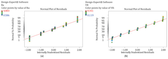
Figure 5.
Normal probability plot (a) arithmetic mean surface roughness, (b) flank wear.
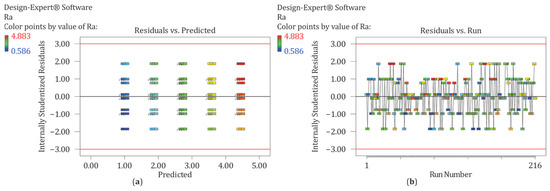
Figure 6.
Arithmetic mean surface roughness internally studentized residuals versus (a) predicted values, (b) run number.
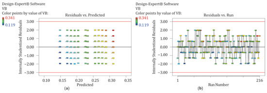
Figure 7.
Flank wear internally studentized residuals versus (a) predicted values, (b) run number.
3.1. Modeling
After conducting experiments and collecting data sets, the development of the ANN model is approached. ANN prediction model based on a feed-forward artificial neural network with a backpropagation training algorithm was developed. The proposed three-layer ANN architecture (Figure 8) has six input parameters and two target parameters. The input data are in the format of 6 × 216, and the target data are in the format of 2 × 216.
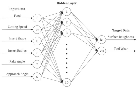
Figure 8.
Architecture of ANN model.
In practice, the optimal number of hidden neurons can be determined using various rules such as rules of thumb [37]: the number of hidden neurons should be between the size of the input layer and the size of the output layer, the number of hidden neurons should be 2/3 the size of the input layer, plus the size of the output layer, the number of hidden neurons should be less than twice the size of the input layer, and rule of pyramid states proposed by Masters [38]. Generally speaking, there is no universal procedure to find an optimal ANN architecture, and the mentioned rules can serve only as good guidelines. For the purposes of this paper, the optimal ANN architecture has been found based on the trial and error method, obeying all the above-mentioned rules.
The model ANN is developed in Matlab within the Deep Learning Toolbox, using the input–output and curve-fitting options. The data set for training consists of 216 samples randomly divided into three parts in a 70:15:15 ratio. The first part with 152 samples was used as an ANN training dataset, the second part with 32 samples was used as a validation dataset, and the third part with 32 samples was used as a test dataset. Mean squared error (MSE) was calculated as a performance measure for all three datasets. We used the Levenberg—Marquardt (LM) algorithm as the training algorithm. Two other available algorithms were also tested (Bayesian Regularization and Scaled Conjugate Gradient Backpropagation), and LM proved to be the best solution in this particular case. This algorithm is also the fastest algorithm and is used for training moderate-sized feed-forward neural networks (up to several hundredweights). More details about this algorithm can be found in [39]. In this study, different architectures and algorithms were tested, and the architecture with four neurons in the hidden layer was chosen as the optimal solution. The regression, performance, and error histogram can be seen in Figure 9.
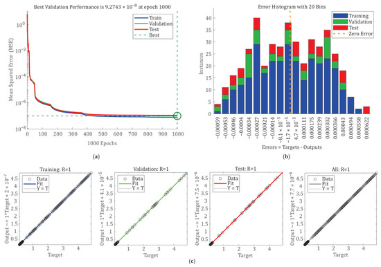
Figure 9.
ANN characteristics (a) performance of optimal architecture, (b) error histogram of optimal architecture, (c) regression of optimal architecture.
The correlation coefficient, which is a measure of how well the variation in output is explained by the targets, is, in this case, R = 1, which confirms that the developed ANN model is well-constructed and trained. Considering that our total correlation factor is 1, we can say that we have an appropriate correlation between the targets and the output data.
The validation of the obtained model was performed by eighteen additional confirmation experiments. The confirmation experiments were performed with combinations of input parameters with which training, testing, and validation of the neural network were not performed. The results obtained and percentage errors are shown in Table 7.
Table 7.
Results of confirmation experiments.
3.2. Optimization
Multi-criteria optimization was performed using a genetic algorithm. The individual objective functions are: minimizing Ra, minimizing VB, and maximizing MRR, so the objective function is accordingly:
where wRa, wVB, wMRR—weight coefficients, an xRa, xVB, xMRR—normalized values of process output parameters. The normalized values of the output process parameters are calculated using the following equations:
The optimization of the presented criteria was implemented in the Matlab program package in the Optimization Toolbox, and the chosen parameters of the genetic algorithm are listed in Table 8.
Table 8.
Optimization parameters.
The following constraints were defined:
- Feed, fopt (mm/rev); fmin ≤ fiopt ≤ fmax; 0.15 ≤ fiopt ≤ 0.25 ∀i∈[1,…,n]; continuous input parameter;
- Cutting speed, vcopt (mm/min); vcmin ≤ vciopt ≤ vcmax; 40 ≤ vciopt ≤ 60 ∀i∈[1,…,n]; continuous input parameter;
- Insert shape, ISopt; ISimin ≤ ISiopt ≤ ISimax; ISiopt = T ∨ S; categorical input parameter;
- Corner radius, riopt (mm); rimin ≤ riopt ≤ rimax; riopt = 0.4 ∨ 0.8 ∨ 1.2; categorical input parameter;
- Rake angle, γiopt (°); γimin ≤ γiopt ≤ γimax; γiopt = 3 ∨ 6 ∨ 9; categorical input parameter;
- Approach angle, κiopt (°); κimin ≤ κiopt ≤ κimax; κiopt = 60 ∨ 75 ∨ 90; categorical input parameter;
- Roughness Raopt (μm); Ramin ≤ Raiopt ≤ Ramax; 0.586 ≤ Raiopt ≤ 4.883 ∀i∈[1,…,n]; continuous output parameter;
- Wear VBopt (mm); VBmin ≤ VBiopt ≤ VBmax; 0.119 ≤ VBiopt ≤ 0.341 ∀i∈[1,…,n]; continuous output parameter;
- Material removal rate, MRRopt (mm3/min rev); MRRmin ≤ MRRiopt ≤ MRRmax; 9 ≤ MRRiopt ≤ 22.5 ∀i∈[1,…,n]; continuous output parameter.
- Four cases were considered in the multi-criteria optimization:
- The output parameters are given equal importance (wRa = 0.33, wVB = 0.33, wMRR = 0.33)—the Ra, VB, and MRR are equally important;
- The output parameters for Ra and VB are given equal importance, and MRR is neglected (wRa = 0.5, wVB = 0.5, wMRR = 0)—the case when the Ra and VB are significant, and MRR is not significant (small production series);
- The output parameters for Ra and MRR are given equal importance, and VB is neglected (wRa = 0.5, wVB = 0, wMRR = 0.5)—the case when the Ra and MRR are significant, and VB is not significant (larger production series and short terms);
- The output parameters of VB and MRR are given equal significance, and Ra is neglected (wRa = 0, wVB = 0.5, wMRR = 0.5)—the case when the VB and MRR are significant, and Ra is not significant (larger production series and short terms).
The obtained results for different values of the weighting factors are presented in Table 9, and the convergence of GA is in Figure 10.
Table 9.
Comparison of optimal and measured parameters.
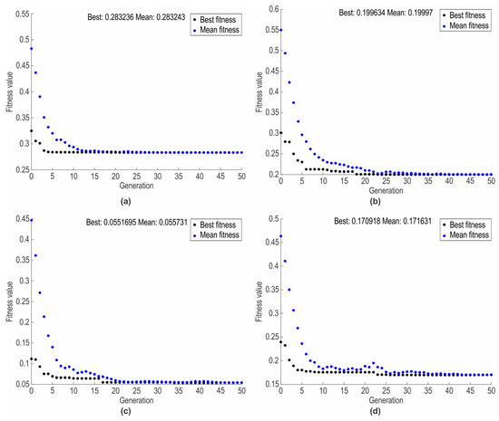
Figure 10.
Convergence of GA (a) wRa = 0.33, wVB = 0.33, wMRR = 0.33; (b) wRa = 0.5, wVB = 0.5, wMRR = 0, (c) wRa = 0.5, wVB = 0, wMRR = 0.5; (d) wRa = 0, wVB = 0.5, wMRR = 0.5.
It is necessary to give some information about the computational time needed for the ANN training and optimization process. The training of the presented ANN model took 0.2 s for 1000 epochs of the training process. As for the optimization process, the computation time depends directly on the number of generations and the population size. Several variations of these parameters were considered, and the parameter values presented in Table 8 were assumed to be optimal. The calculation time for these parameters was 58 s. All calculations were performed using a computer configuration with a 2.4 GHz processor and 8 GB RAM. Finally, we must emphasize that all calculations must be performed only once, and the obtained ANN model and optimal parameter values can be used for all further work, so the system does not work in real-time, and the speed of calculation is not crucial for the performance of the presented solutions.
Additional confirmation experiments were performed for the optimal input parameters. The measured values of the output parameters are close to the values computed using the optimal input parameters. The percentage errors obtained are below 2%, which demonstrates the possibility of optimizing the input parameters in the context of a practical application under real production conditions.
4. Discussion
When feed increases, roughness and wear increase, and vice versa. When the feed is increased, wider and higher peaks and valleys appear on the surface of the workpiece, which affects the increase in surface roughness. Increasing the feed has the effect of increasing the cutting forces, which directly affects the increase in flank wear. As cutting speed increases, surface roughness decreases and flank wear increases, and vice versa. As the cutting speed increases, the cutting forces decrease, and the cutting temperature increases. The result of the temperature increase is higher flank wear. At the same time, the flank wear does not reach a critical level, so it does not have a negative effect on the surface roughness, i.e., it increases the surface roughness. The “S” insert shape produces less surface roughness and less flank wear. This insert shape distributes the heat better over the cutting edge and thus causes a reduction in flank wear and surface roughness. As the corner radius increases, surface roughness and wear decrease, and vice versa. When the corner radius increases on the surface of the workpiece, lower valleys and peaks result, which affects the reduction of surface roughness. With larger corner radii, the length of contact between the cutting insert and the workpiece increases. This distributes heat over a larger surface area and reduces flank wear. With an increase in rake angle, flank wear increases, while surface roughness initially decreases and then increases. An increase in the rake angle causes a weakening of the cutting edge, i.e., a reduction in the strength of the cutting insert resulting in increased flank wear. With an increase in the rake angle, cutting forces decrease due to a larger shear angle, allowing the cutting insert to penetrate the workpiece more easily, which helps to reduce flank wear until a certain temperature is reached in the cutting zone. However, with a further increase in rake angle due to a higher temperature in the cutting zone and a decrease in cutting insert strength, the flank wear worsens. As the approach angle increases, the surface roughness decreases, and the flank wear of the cutting insert increases. When the approach angle increases, the width of the chip increases as the overall length of the cutting edge increases. This contributes to better heat dissipation from the cutting zone, which leads to a reduction in flank wear and, thus, in surface roughness.
The high temperatures encountered during the dry turning of Inconel alloys can increase cutting insert wear. The TiAlN coating has a good anti-friction effect and thermal barrier effect, thus improving the cutting performance [40]. The titanium aluminum nitride multilayer coatings used in the study have high hardness combined with oxidation resistance, which improves the overall wear resistance. This contributes to acceptable flank wear values even at higher cutting speeds.
The obtained optimization results show that regardless of the importance of certain output parameters, three input parameters are always identical, namely: the insert shape (square), the corner radius (maximum level), and the approach angle (minimum level). This is due to the fact that square-cutting inserts with a larger corner radius flank wear more slowly and, at the same time, produce a surface with lower roughness without affecting the amount of material removed per unit of time. Other input parameters vary from case to case.
In the first case (wRa = 0.33, wVB = 0.33, wMMR = 0.33), the feed is at the maximum level (0.25 mm/rev), the cutting speed is close to the maximum level (56 mm/min), and the rake angle is at the middle level (γ = 6°). This is due to the fact that cutting speed and feed have a directly proportional effect on the increase in material removal rate. The cutting speed had a small effect on the surface roughness and a significant one on the flank wear, but its influence was compensated by a compromise with other input parameters (IS, r, γ, κ) that have a positive influence on the flank wear of the cutting insert. The feed has a small effect on the flank wear and a significant effect on the surface roughness, but its influence is compensated by a compromise with other input parameters (IS, r, κ) that have a positive influence on the surface roughness. The middle level of the rake angle (γ = 6°) produces the lowest surface roughness.
In the second case (wRa = 0.5, wVB = 0.5, wMMR = 0), the cutting speed (40 mm/min) and the feed (0.25 mm/rev) are the lowest, and the rake angle is at the middle level (γ = 6°). This is a consequence of the fact that, in this case, Ra and VB are the smallest.
In the third case (wRa = 0.5, wVB = 0, wMMR = 0.5), the feed (0.25 mm/rev) and the cutting speed (60 mm/rev) are at the maximum level, and the rake angle is at the middle level (γ = 6°). This is due to the fact that cutting speed and feed have a directly proportional effect on the increase in material removal rate. The cutting speed has only a minor influence on the surface roughness. The feed has a significant influence on the surface roughness, but its influence is compensated by compromise with other input parameters (IS, r, γ, κ) that have a positive influence on the surface roughness. The middle level of the rake angle (γ = 6°) produces the lowest surface roughness.
In the fourth case (wRa = 0, wVB = 0.5, wMMR = 0.5), the feed is at the maximum level (0.25 mm/rev), the cutting speed (55 mm/min) is close to the maximum level, and the rake angle is at the minimum level (γ = 3°). This is due to the fact that cutting speed and feed have a directly proportional effect on the increase in material removal rate. The feed has had a minor influence on the flank wear. The cutting speed has a significant influence on the flank wear, but its influence is compensated by compromise with other input parameters (IS, r, γ, κ) that have a positive influence on the flank wear. A smaller rake angle (γ = 3°) reduces the flank wear.
5. Conclusions
In this paper, the modeling and optimization of the machining parameters and the geometry of the cutting insert were performed from the point of view of the quality of the machined surface, tool life, and productivity.
With an appropriate choice of input parameters, the output parameters can be obtained in a wide range, namely: Ra = 0.586–4.883 µm, VB = 0.119–0.341 mm, and MRR = 9–22.5 mm3/min. This is very important from the point of view of practical application when it comes to obtaining the required output parameters.
Based on the results obtained, some general conclusions can be drawn: increasing the feed has a positive effect on MRR and a negative effect on Ra and VB; increasing the cutting speed has a positive effect on MRR and RA and a negative effect on VB; the square shape of the cutting insert has a positive effect on Ra and VB; increasing the radius of the cutting insert has a positive effect on Ra and VB; increasing the approach angle has a negative effect on Ra and VB; increasing the rake angle has a negative effect on VB, and it first has a positive effect on Ra and then a negative effect on Ra.
The optimal combinations of input process parameters vary with the requirements of the defined importance of the output process parameters. Different optimal combinations of optimal input parameters are obtained for different ratios of the importance of machined surface quality, tool life, and productivity. The obtained results show that it is favorable to perform machining with a larger corner radius and a square shape of the cutting inserts, as well as with a smaller approach angle, regardless of other production requirements.
The percentage optimization errors are in the range of 0.260–1.112% for Ra and in the range of 1.527–1.807% for VB. These percentage errors correspond to absolute errors in the range of 0.006–0.027 µm for Ra and in the range of 0.002–0.004 mm for VB. The obtained errors show the possibility of practical implementation of the proposed methodology in a real production environment.
It should be noted that the research has certain limitations, based on which future research can be defined. The obtained results can be applied to the conditions in which the experiments were conducted. In order to achieve greater universality of the developed model, experimental studies are planned on workpieces with different mechanical, physical, and thermal properties, as well as on tools with different geometrical and technological characteristics. Future research directions will also focus on modeling and optimizing a larger number of parameters, i.e., incorporating a larger number of input parameters (depth of cut, clearance angle, inclination angle, properties of the coating, etc.) and output parameters of the process (hardness, residual stresses, etc.) with other modeling and optimization methods. Finally, future research is planned to investigate wear mechanisms, wear patterns, wear morphology, structural changes, and mechanical properties of the workpiece.
Author Contributions
Conceptualization, G.J., Z.K. and D.V.; methodology, G.J., A.M., B.S. and D.V.; software, G.J., Z.K. and G.S.; validation, G.J., A.M. and M.S.; formal analysis, Z.K., G.S. and D.V.; investigation, A.M., M.S. and B.S.; resources, A.M., M.S. and B.S.; visualization, G.S.; writing—original draft, G.J., A.M., Z.K., M.S., G.S. and B.S.; writing—review and editing, D.V.; supervision, D.V. All authors have read and agreed to the published version of the manuscript.
Funding
This research was funded by the Ministry of Science, Technological Development and Innovation of the Republic of Serbia, grant number 451-03-47/2023-01/200156, and by the University of Slavonski Brod, Mechanical Engineering Faculty in Slavonski Brod, Republic of Croatia, grant number SV001.
Data Availability Statement
Not applicable.
Conflicts of Interest
The authors declare no conflict of interest.
References
- Dudzinski, D.; Devillez, A.; Moufki, A.; Larrouquere, D.; Zerrouki, V.; Vigneau, J. A review of developments towards dry and high speed machining of Inconel 718 alloy. Int. J. Mach. Tools Manuf. 2004, 44, 439–456. [Google Scholar] [CrossRef]
- Ezugwu, E.O.; Wang, Z.M.; Machado, A.R. The machinability of nickel-based alloys: A review. J. Mater. Process. Technol. 1999, 86, 1–16. [Google Scholar] [CrossRef]
- Danish, M.; Gupta, M.K.; Rubaiee, S.; Ahmed, A.; Sarıkaya, M.; Krolczyk, G.M. Environmental, technological and economical aspects of cryogenic assisted hard machining operation of inconel 718: A step towards green manufacturing. J. Clean. Prod. 2022, 337, 130483. [Google Scholar] [CrossRef]
- Li, L.; He, N.; Wang, M.; Wang, Z.G. High speed cutting of Inconel 718 with coated carbide and ceramic inserts. J. Mater. Process. Technol. 2002, 129, 127–130. [Google Scholar] [CrossRef]
- Devillez, A.; Schneider, F.; Dominiak, S.; Dudzinski, D.; Larrouquere, D. Cutting forces and wear in dry machining of Inconel 718 with coated carbide tools. Wear 2007, 262, 931–942. [Google Scholar] [CrossRef]
- Nalbant, M.; Altin, A.; Gokkay, A.H. The effect of cutting speed and cutting tool geometry on machinability properties of nickel-base Inconel 718 super alloys. Mater. Des. 2007, 28, 1334–1338. [Google Scholar] [CrossRef]
- Outeiro, J.C.; Pina, J.C.; M’Saoubi, R.; Pusavec, F.; Jawahir, I.S. Analysis of residual stresses induced by dry turning of difficult-to-machine materials. CIRP Ann. 2008, 57, 77–80. [Google Scholar] [CrossRef]
- Attia, H.; Tavakoli, S.; Vargas, R.; Thomson, V. Laser-assisted high-speed finish turning of superalloy Inconel 718 under dry conditions. CIRP Ann.-Manuf. Technol. 2010, 59, 83–88. [Google Scholar] [CrossRef]
- Akhyar Ibrahim, G.; Che Haron, C.H.; Abdul Ghani, J.; Said, A.Y.M.; Abu Yazid, M.Z. Performance of PVD-coated carbide tools when turning Inconel 718 in dry machining. Adv. Mech. Eng. 2011, 790975. [Google Scholar] [CrossRef]
- Umbrello, D. Investigation of surface integrity in dry machining of Inconel 718. Int. J. Adv. Manuf. Tech. 2013, 69, 2183–2190. [Google Scholar] [CrossRef]
- Ramanujam, R.; Venkatesan, K.; Saxena, V.; Joseph, P. Modeling and Optimization of Cutting Parameters in Dry Turning of Inconel 718 using Coated Carbide Inserts. Procedia Mater. Sci. 2014, 5, 2550–2559. [Google Scholar] [CrossRef]
- Ramanujam, R.; Venkatesan, K.; Saxena, V.; Pandey, R.; Harsha, T.; Kumar, G. Optimization of machining parameters using fuzzy based principal component analysis during dry turning operation of inconel 625—A hybrid approach. Procedia Eng. 2014, 97, 668–676. [Google Scholar] [CrossRef]
- Satyanarayana, B.; Yadav, G.S.G.; Nitin, P.R.; Reddy, M.D. Simultaneous Optimization of Multi Performance Characteristics in Dry Turning of Inconel 718 Using NSGA-II. Mater. Today 2015, 2, 2423–2432. [Google Scholar] [CrossRef]
- Thakur, A.; Gangopadhyay, S.; Mohanty, A. Investigation on some machinability aspects of inconel 825 during dry turning. Mater. Manuf. Process. 2015, 30, 1026–1034. [Google Scholar] [CrossRef]
- Thakur, A.; Gangopadhyay, S. Dry machining of nickel-based super alloy as a sustainable alternative using TiN/TiAlN coated tool. J. Clean. Prod. 2016, 129, 256–268. [Google Scholar] [CrossRef]
- Vetri Velmurgan, K.; Venkatesan, K. An investigation of the parametric effects of cutting parameters on quality characteristics during the dry turning of inconel 718 alloy. Indian J. Sci. Technol. 2016, 9, 103314. [Google Scholar] [CrossRef]
- Liu, J.; Ma, C.; Tu, G.; Long, Y. Cutting performance and wear mechanism of Sialon ceramic cutting inserts with TiCN coating. Surf. Coat. Technol. 2016, 307, 146–150. [Google Scholar] [CrossRef]
- Zeilmann, R.P.; Fontanive, F.; Soares, R.M. Wear mechanisms during dry and wet turning of Inconel 718 with ceramic tools. Int. J. Adv. Manuf. Technol. 2017, 92, 2705–2714. [Google Scholar] [CrossRef]
- Thakur, A.; Gangopadhyay, S. Evaluation of micro-features of chips of Inconel 825 during dry turning with uncoated and chemical vapour deposition multilayer coated tools. Proc. Inst. Mech. Eng. Part B J. Eng. Manufact. 2018, 232, 979–994. [Google Scholar] [CrossRef]
- Cantero, J.L.; Díaz-Álvarez, J.; Infante-García, D.; Rodríguez, M.; Criado, V. High Speed Finish Turning of Inconel 718 Using PCBN Tools under Dry Conditions. Metals 2018, 8, 192. [Google Scholar] [CrossRef]
- Hua, Y.; Liu, Z. Effects of cutting parameters and tool nose radius on surface roughness and work hardening during dry turning Inconel 718. Int. J. Adv. Manuf. Technol. 2018, 96, 2421–2430. [Google Scholar] [CrossRef]
- Qiu, X.; Cheng, X.; Dong, P.; Peng, H.; Xing, Y.; Zhou, X. Sensitivity Analysis of Johnson-Cook Material Constants and Friction Coefficient Influence on Finite Element Simulation of Turning Inconel 718. Materials 2019, 12, 3121. [Google Scholar] [CrossRef] [PubMed]
- Hemakumar, S.; Kuppan, P. Experimental investigations and optimisation of process parameters in dry finish turning of Inconel 625 super alloy. Int. J. Mater. Prod. Technol. 2019, 59, 303–320. [Google Scholar] [CrossRef]
- Shalaby, M.A.; Veldhuis, S.C. Tool wear and chip formation during dry high speed turning of direct aged Inconel 718 aerospace superalloy using different ceramic tools. Proc. Inst. Mech. Eng. Part J J. Eng. Tribol. 2019, 233, 1127–1136. [Google Scholar] [CrossRef]
- Qadria, S.I.A.; Harmain, G.A.; Wani, M.F. Influence of Tool Tip Temperature on Crater Wear of Ceramic Inserts During Turning Process of Inconel-718 at Varying Hardness. Tribol. Ind. 2020, 42, 310–326. [Google Scholar] [CrossRef]
- Zhao, J.; Liu, Z. Influences of coating thickness on cutting temperature for dry hard turning Inconel 718 with PVD TiAlN coated carbide tools in initial tool wear stage. J. Manuf. Process 2020, 56, 1155–1165. [Google Scholar] [CrossRef]
- Peng, H.; Dong, P.; Cheng, X.; Zhang, C.; Tang, W.; Xing, Y.; Zhou, X. Semi-Empirical Prediction of Residual Stress Distributions Introduced by Turning Inconel 718 Alloy Based on Lorentz Function. Materials 2020, 13, 4341. [Google Scholar] [CrossRef]
- Vukelic, D.; Simunovic, K.; Simunovic, G.; Saric, T.; Kanovic, Z.; Budak, I.; Agarski, B. Evaluation of an environment-friendly turning process of Inconel 601 in dry conditions. J. Clean. Prod. 2020, 266, 121919. [Google Scholar] [CrossRef]
- Ren, X.; Liu, Z.; Liang, X.; Cui, P. Effects of Machined Surface Integrity on High-Temperature Low-Cycle Fatigue Life and Process Parameters Optimization of Turning Superalloy Inconel 718. Materials 2021, 14, 2428. [Google Scholar] [CrossRef]
- Veerappan, G.; Pritima, D.; Parthsarathy, N.R.; Ramesh, B.; Jayasathyakawin, S. Experimental investigation on machining behavior in dry turning of nickel based super alloy-Inconel 600 and analysis of surface integrity and tool wear in dry machining. Mater. Today 2022, 59, 1566–1570. [Google Scholar] [CrossRef]
- Yashwant Bhise, V.; Jogi, B.F. Effect of cutting speed and feed on surface roughness in dry turning of Inconel X-750. Mater. Today 2022, 61, 587–592. [Google Scholar] [CrossRef]
- Zhao, J.; Liu, Z.; Wang, B.; Qinhuq, S.; Xiaoping, R.; Wan, Y. Effects of Al content in TiAlN coatings on tool wear and cutting temperature during dry machining IN718. Tribol. Int. 2022, 171, 107540. [Google Scholar] [CrossRef]
- Xue, C.; Wang, D.; Zhang, J. Wear Mechanisms and Notch Formation of Whisker-Reinforced Alumina and Sialon Ceramic Tools during High-Speed Turning of Inconel 718. Materials 2022, 15, 3860. [Google Scholar] [CrossRef]
- Szablewski, P.; Legutko, S.; Mróz, A.; Garbiec, D.; Czajka, R.; Smak, K.; Krawczyk, B. Surface Topography Description after Turning Inconel 718 with a Conventional, Wiper and Special Insert Made by the SPS Technique. Materials 2023, 16, 949. [Google Scholar] [CrossRef] [PubMed]
- Grigoriev, S.; Vereschaka, A.; Uglov, V.; Milovich, F.; Cherenda, N.; Andreev, N.; Migranov, M.; Seleznev, A. Influence of tribological properties of Zr-ZrN-(Zr,Cr,Al)N and Zr-ZrN-(Zr,Mo,Al)N multilayer nanostructured coatings on the cutting properties of coated tools during dry turning of Inconel 718 alloy. Wear 2023, 512–513, 204521. [Google Scholar] [CrossRef]
- Dhananchezian, M. Surface roughness and insert wear in turning Ti-6Al-4 V and Inconel 600 alloys with tungsten carbide inserts under dry conditions. Mater. Today 2023, 72, 2118–2124. [Google Scholar] [CrossRef]
- Panchal, F.S.; Panchal, M. Review of selecting Number of Hidden Nodes in Artificial Neural Networks. Int. J. Comput. Sci. Mob. Computing 2014, 3, 455–464. [Google Scholar]
- Masters, T. Practical Neural Network Recipies in C++; Academica Press: San Diego, CA, USA, 1993. [Google Scholar]
- Marquardt, W.D. An Algorithm for Least-Squares Estimation of Nonlinear Parameters. SIAM J. Appl. Math. 1963, 11, 431–441. [Google Scholar] [CrossRef]
- Zhao, J.; Liu, Z.; Wang, B.; Hu, J.; Wan, Y. Tool coating effects on cutting temperature during metal cutting processes: Comprehensive review and future research directions. Mech. Syst. Signal Process. 2021, 150, 107302. [Google Scholar] [CrossRef]


Disclaimer/Publisher’s Note: The statements, opinions and data contained in all publications are solely those of the individual author(s) and contributor(s) and not of MDPI and/or the editor(s). MDPI and/or the editor(s) disclaim responsibility for any injury to people or property resulting from any ideas, methods, instructions or products referred to in the content. |
© 2023 by the authors. Licensee MDPI, Basel, Switzerland. This article is an open access article distributed under the terms and conditions of the Creative Commons Attribution (CC BY) license (https://creativecommons.org/licenses/by/4.0/).