Abstract
This paper used the smoothed particle hydrodynamics (SPH) method to construct a three-dimensional mathematical model of the selective laser melting (SLM) process of 304 L austenitic stainless steel. Important driving force models for the melt pool in the SLM process were developed, including a surface tension model, a boundary normal-modified wetting effect model, a Marangoni shear force model, and a recoil pressure model. Meanwhile, the virtual particle boundary method prevented particles from flying over the solid boundary. Artificial viscosity, artificial stress, and artificial heat were added to correct the SPH equation, which provided a guarantee for the accuracy and speed of the numerical simulation of the SLM process. Finally, the temperature field and velocity field in the SLM process were explored according to the constructed mathematical model. The evolution mechanism in the melting process was analyzed, and the influence of different laser powers on the shape of the molten pool was mainly analyzed, which provided a reference for optimizing the laser parameters to reduce the surface roughness of the formed specimen.
1. Introduction
During the SLM process, various complex physical phenomena are involved between powder layers, within the molten pool, and during the solidification phase. In the SLM process, parameters such as the laser power, powder layer thickness, and scanning speed will affect the shape of the melt pool, crystal defects, and microstructure, affecting the final performance of the printed part [1,2]. Therefore, a clear understanding of the relationship between parameters, structure, and performance is essential for producing high-quality products. In instances where the scanning velocity is elevated, and the laser potency is inadequate, the energy absorbed by the powder proves insufficient to achieve complete liquefaction, thereby yielding a diminished density in the fabricated component. Conversely, when both the scanning velocity and laser potency are relatively elevated, the augmented depth of the laser penetration facilitates the ingress of the shielding gas into the molten state, consequently leading to keyhole imperfections [3,4,5].
In 2015, Lee and Zhang [6] devised a three-dimensional dynamic numerical framework for LPBF additive manufacturing, considering the impact of Marangoni shearing forces. Biegler et al. [7] investigated the phenomenon of component deformation during directional energy deposition (DED) additive manufacturing (AM) due to repeated local heating. Quantitative studies were conducted on laser power, scan speed, and powder particle size distribution affecting the final quality of the prints. Moreover, the fluid volume method and discrete element method were used to analyze and calculate the placement of individual metal powders, respectively, considering the arrangement of powder particles, including particle size distribution and bulk density. The findings [8,9] demonstrate that an asymmetrically skewed distribution of particle sizes, characterized by a substantial abundance of smaller particles, will render the contour of the molten pool more uniform; augmenting the scanning velocity while diminishing the laser intensity will heighten the likelihood of generating spheroidization flaws; nevertheless, the path traversed by the laser remains relatively unexplored. In 2015, M.A. Russell and A. Souto-Iglesias [10] pioneered the employment of the SPH technique to precisely resolve the thermal and mechanical properties and the material fields in the context of laser-based three-dimensional printing. This work validated a novel formula based on the smoothed particle hydrodynamics (SPH) technique, employing an isothermal and incompressible fluid model. This formula enables precise simulation of the expansion and contraction phenomena experienced by liquid-phase metals under the influence of thermal forces. However, the model neglects the impact of thermal expansion, vaporization, and regular surface tension on the deposition process.
The properties of the SPH method make it easy to solve problems related to complex models, free-surface flows, and multiphase flows, which exactly suit the case when the melt interacts with the shielding gas in the SLM process [11,12,13,14]. Considering the advantages of the SPH method, some foreign scholars tried to use the SPH method to simulate the SLM process. M.A. Russell et al. [10] spearheaded the development of a relatively comprehensive mathematical framework for the selective laser melting (SLM) procedure, investigating the impact of laser energy on the configuration of the molten pool. Nonetheless, their inquiry was confined to a two-dimensional realm. Scant domestic researchers have embraced the smoothed particle hydrodynamics (SPH) approach to resolve the complexities of the SLM process. In a similar vein, Qiu Yunji et al. [15,16] devised a mathematical model grounded in the SPH methodology to corroborate SPH’s applicability in simulating SLM. However, the employed powder bed model assumes an idealized arrangement of a single row of powder, deviating from real-world scenarios. Consequently, this study leverages the SPH method and employs a randomized powder bed model to undertake a numerical simulation investigation of the SLM process for 304 L.
2. Basic Theory and Model of SPH Method
2.1. Construction of the SPH Equation
The construction of the SPH equation is generally divided into two steps: first, approximate the continuous field function as an integral expression related to the kernel function, and then use the particle approximation method to discretize the integral expression obtained in the previous step as the superposition and summation of adjacent particles form [17,18].
2.1.1. Integral Notation
Integral representation focuses on the stepwise integration of arbitrary and smooth functions using the kernel approximation of integral representation functions. If the field function f(r) of a point in the solution domain satisfies the defined and continuous conditions, it can be written in the following form:
where r is the space position vector, is the space position vector, and is the Dirac function.
Using a smooth function with similar properties to replace the Dirac function, the function can be approximated as
where represents the smooth function, and h represent the distance between two points and the smooth length, respectively.
The transformation from Formula (2) can be obtained:
In Formula (3), the kernel function has a non-zero calculation result in the support domain. In the process of solving the divided problem domain, there may be the following situations: the kernel function is wholly located in its support domain, the calculation result of the kernel function is not zero at this time, and the integral of the first area integral term on the right side of Equation (3) is zero, and Formula (3) can be represented by Formula (4).
2.1.2. Particle Approximation
In the simulation calculation program developed based on the SPH method, the limited number of particles divided by the problem domain at the initial moment have independent masses and occupy independent spaces, which are obtained by the particle approximation method and transform the integral expression of continuous field function approximation into the sum of all particles in the solution domain. Then, the mass of the particle can be expressed as
where represents the volume and represents the density, j = (1, 2, …, N), N is the sum of the number of SPH particles in the problem domain.
The particle approximation result of Equation (2) is listed as follows:
Finally, the particle approximation at particle i can be expressed as
The final particle approximation of the field function can be expressed as
2.2. Fluid Control Equations
Laser-selective melting (SLM) uses a high-energy laser to melt a metal powder laid on a predetermined path to form a liquid melt pool and then solidify it into shape. In the SPH method, the motion of this weakly compressible fluid used to describe this SLM process is controlled by the Navier–Stokes equations.
The Navier–Stokes equations for the motion of incompressible fluid are
Using the SPH method described in Section 2.1, the above equations can be discretized into the following form:
where and represent the hydrostatic pressure and kinematic viscosity coefficients, respectively. P represents the pressure, and u represents the scale factor. is the surface tension. N represents the total number of particles contained in the support domain of particle i, is the mass of particle j, and is the smooth function at particle j, which is approximated by a weighted average of the function values corresponding to all particles in the support domain.
2.3. Modified SPH Equation
2.3.1. Artificial Viscosity
The simulation calculation in this paper adopts the most widely used Monaghan artificial viscosity model [19], and its expression is as follows:
where
is used to ensure that the calculated value does not diverge, and are standard constants, represents the speed of particles, and c represents the speed of sound. The momentum equation considering artificial viscosity is
2.3.2. Artificial Stress
When the classical SPH method is used to solve the second derivative of SPH, it is very easy to produce low accuracy and tensile instability. For more accurate and stable calculation results, the artificial stress method was proposed by Monaghan [19] and Gray [20]. The core of this method is that when the particles approach each other and exceed a certain limit distance, a small reverse repulsive force is artificially imparted to the particles close to each other to prevent the particles from getting too close and agglomerating. The expression is
In the formula, , represents the distance between the i particle and the j particle, represents the distance between the initial particles. , where and are not conventional physical quantities but are artificial parameters that depend on density and pressure.
where and are both taken as 0.2.
2.3.3. Artificial Heat
In this paper, artificial heat is introduced to modify the energy conservation equation, and its expression is as Formula (24):
where
In the above formula, the value of the standard constants and are the same as the artificial viscosity, so the energy conservation equation of the SPH method with artificial heat added can be expressed as
2.4. SPH Solid Wall Boundary Conditions
In the process of simulating SLM, the laser gives energy to the powder bed to form a molten pool, and the melted powder driven by surface tension will generate a tangential viscous flow with the substrate, so the setting of virtual particles can effectively solve the viscous force between the two [21]. The boundary governing equations used in this paper are as follows:
In the above formula, is the pressure of the boundary particles, is the pressure of the internal fluid particles, represents the smooth kernel function. is the acceleration of the boundary particle, and is the space vector of the distance between the boundary particle and the fluid particle.
When applying boundary conditions, it is possible to apply free-slip conditions while ignoring the viscous interactions of fluid particles with adjacent virtual particles. In the simulation of the SLM process, a non-slip boundary condition is applied, and the fluid phase is first transferred to the virtual particle position by extrapolating the smoothed velocity field by the Equation (21):
Therefore, the velocity of the boundary particle is listed as Formula (29):
where is the velocity of the motion boundary.
In this process, we do not need the boundary particles to evolve the density, and the density value of the boundary particles themselves can be solved in the process of simulating according to the following formula:
2.5. Surface Tension and Wetting Effect
2.5.1. Surface Tension Model
During the numerical simulation of the SLM process, the continuous surface force (CSF) model [22] is employed, incorporating the utilization of the color function to facilitate the conversion from surface force to body force:
wherein n corresponds to the normalized unit vector of the interface while denotes the coefficient of surface tension. signifies the curvature of the interface, and is a function that relates to the tangential orientation of the surface [23].
The final expression for the surface tension is obtained after deformation as follows:
2.5.2. Wetting Effect
The force of the droplet on the solid wall can be expressed by Young’s equation:
where is the solid–liquid surface tension and is the solid–gas surface tension. The deformation of Formula (33) can be obtained as
where represents the contact angle, represents the equilibrium contact angle, and when the two are equal, the droplet reaches dynamic equilibrium.
2.6. Marangoni Shear Force
While formulating the mathematical framework for the selective laser melting process in this study, the acknowledgment is made that the interaction between the liquid molten pool and the shielding gas gives rise to the manifestation of surface tension and Marangoni shear force. The Marangoni shear force model in SPH format is introduced [10]: If you want to simulate the Marangoni shear force, you need to calculate the thermal gradient first:
The Marangoni shear force is calculated using the expression for the thermal gradient:
where represents the renormalization factor, is the surface tension coefficient, and n is the interface unit normal.
2.7. Backlash Pressure
The vapor recoil pressure imparts supplementary force onto the liquid surface, resulting in a depression within the molten pool beneath the laser. As the heating employed in the L-PBF process does not induce extensive vaporization (ablation), the current model does not incorporate considerations for the abruptness and expansion of the vapor flow as it transitions from the liquid phase to the surrounding gas [24], nor does it encompass the loss of mass due to evaporation. The recoil pressure can be effectively elucidated by adopting the simplified model proposed by Anisimov [25]:
3. Model Verification and Experimental Results
3.1. Validation Example of Wall Droplet Wetting Effect Model
Throughout the selective laser melting process, the dynamics of the molten pool formation are profoundly influenced by the interplay of surface tension and wetting phenomena. These factors play a crucial role in determining the morphology of the molten pool. To ensure favorable wetting behavior, the equilibrium contact angle between the metal powder and the substrate of 304 stainless steel was established at 45° [26].
The wetting effect model was validated through a three-dimensional droplet evolution example. The geometric and physical model, and its dimensions, is depicted in Figure 1. The outermost shell represents the solid wall boundary, the deep blue region represents the solid substrate, the yellow spherical objects represent the oil droplets, and the surrounding medium is a water solution. The boundary and substrate are virtual particles, with a total count of 117,388, while the oil droplets and water solution are represented as fundamental particles, with a total count of 186,184. Hence, the total particle count is 303,572. The wetting contact angle is 45 degrees, and the surface tension is 0.050475 N/m. Because gravity is not the primary force considered in this context, it is not considered.
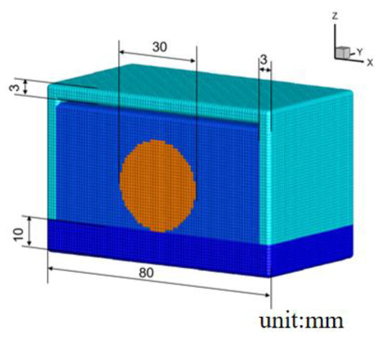
Figure 1.
A three-dimensional physical model for calculating the natural evolution of initial spherical oil droplets on the wall.
Figure 2 shows the evolution results of the three-dimensional droplet. The system is in a static state at the initial moment. When t = 0.01 s, because the interface normal is corrected at the three-phase junction, the surface tension points to both sides, and the direction is upward, and then the droplet begins to contact the wall and expand to the surrounding simultaneously. At the junction of the droplet and the solid wall, there is a concave arc toward the inside of the droplet; at this time, the speed of the middle part of the droplet is downward, and a vortex is formed on both sides, as shown in Figure 3a. Subsequently, under the combined influence of external and internal forces, the interface area between the solid wall and the liquid surface undergoes continuous enlargement while the droplet height steadily diminishes. This progression is accompanied by an escalation in the velocity field’s vortex, and the droplet section’s particle velocity in contact with the wall tends to extend horizontally toward both sides, as depicted in Figure 3b. At t = 0.15 s, the equilibrium contact angle is achieved, signifying that the contact area between the solid wall and the liquid surface no longer experiences any further augmentation. Furthermore, the droplet height reaches its minimum, thus attaining a state of dynamic equilibrium. Consequently, this three-dimensional droplet evolution exemplar validates the accuracy of the surface tension and wetting effect models within the mathematical framework of the SLM process.

Figure 2.
Three-dimensional numerical simulation of the process of oil droplets wetting the wall surface in aqueous solution at θ = 45°.
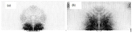
Figure 3.
Three-dimensional numerical simulation of the wetting process of oil droplets in aqueous solution at different times: (a) t = 0.01 s; (b) t = 0.07 s.
3.2. SPH Numerical Simulation Results and Analysis
3.2.1. Thermophysical Parameters of 304 L Austenitic Stainless Steel
In this paper, 304 L austenitic stainless steel with relatively complete thermophysical parameters is selected, and some thermophysical parameters of its powder are shown in Table 1.

Table 1.
Partial thermophysical parameters of 304 L metal powder data from [27,28].
3.2.2. Random Powder Bed Model
In this paper, the random powder bed modeling of the metal powder bed in the SLM process is carried out by the discrete element method. The parameters are shown in Table 2. The powder bed model is shown in Figure 4.
Table 2.
Modeling parameters for random powder beds.

Figure 4.
The powder bed model.
3.2.3. SPH Simulation Results
Figure 5 illustrates the topographic evolution of the selective laser melting (SLM) process at 4 distinct time points, with the laser power set at 150 W. As depicted in the figure, when the t = 0.02 s, the metal powder particles undergo complete liquefaction due to the laser irradiation, resulting in forming an elliptical, high-temperature molten pool. Notably, the neighboring powder exhibits a lower initial temperature and absorbs a lesser amount of laser energy, thereby leading to the emergence of a significant temperature gradient. As the laser scanning time progresses, the surrounding powder and the substrate experience a gradual temperature rise owing to the influence of thermal conduction. The area gradually expands. This is because Marangoni convection drives the melt flow from the high temperature of the laser irradiation point to the lower temperature behind it. This helps to increase the melt depth, allowing the melt flow to reflow, thereby cooling the location of the laser spot. This surface flow leads to recirculation vortices that expand the size of the melt pool by increasing fluid convection. When t = 0.08 s, the pool trajectory stabilizes, and the pool edge has solidified and deposited, completing the simulation of this channel.
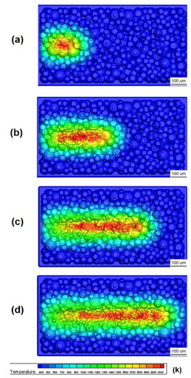
Figure 5.
Schematic diagram of SPH simulation results when P = 150 W: (a) t = 0.02 s, (b) t = 0.04 s, (c) t = 0.06 s, (d) t = 0.08 s.
In the lower region of the molten pool, an excessive disparity in temperature distribution gives rise to a decline in the surface tension gradient. Consequently, the molten metal and solute migrate from regions with lower surface tension to areas with higher surface tension. Moreover, the surface tension gradient-induced instability in the fluid flow within the molten pool exacerbates this phenomenon. As a result, an uneven surface topography ensues, accompanied by fluid oscillations and an expansion in the width of the molten pool. In this paper, the X-Z plane of the simulation results of the SPH software is selected for research, and the (a) temperature field and (b) velocity field in Figure 6 are observed. It can be seen that the molten metal at the molten pool has a velocity opposite to that of the laser scanning direction, and the more near the molten pool the velocity is, the more remarkable; however, the molten metal at the edge of the molten pool has a backflow velocity. This is because the Marangoni convection drives the melt flow from the high temperature of the laser irradiation point to the lower temperature behind it [29]. This helps to increase the melt depth, allowing the melt flow to reflow, thereby cooling the location of the laser spot, during which the low-viscosity liquid metal is ejected from the surface. These will have a significant influence on the morphology of the molten pool.

Figure 6.
Temperature and velocity fields of the melt pool.
The metal melt pool expansion driven by Marangoni convection can be observed by looking at the (Figure 6a) temperature field and (Figure 6b) velocity field of the molten pool in Figure 6. At the same time, the high-temperature molten metal at the bottom of the molten pool moves downward, because the recoil pressure gives the liquid surface a downward velocity, resulting in a depression on the surface of the molten pool. Through the combination of Marangoni convection and recoil pressure, the melt depth and surface area are significantly increased while additional surface evaporation and radiation further reduce the temperature of the melt pool. It is under the action of Marangoni convection and recoil pressure that the molten pool morphology shown in Figure 5 is formed. These verify the correctness of the back-punching procedure written in the software and that Marangoni convection plays an essential role in the morphology of the molten pool during SLM.
In this paper, we simulate the SLM process at a laser power of 100 W, 150 W, and 200 W and a scanning speed of 15 cm/s. Other parameter settings of the simulation process are referred to in Table 1 and Table 2. As shown in Figure 7, it can be observed that the width of the molten pool gradually increases with the increase in the laser power. At lower laser power, the temperature gradient of the molten pool is small, the cooling rate of the molten pool is faster, and the molten pool is relatively stable [30,31]. This can result in poor powder and substrate wettability, spheroidization, and discontinuous solidified melt. When the power is too high, the volume of the molten pool expands greatly. At this time, the Marangoni convection significantly affects the morphology of the molten pool, and the molten pool is disturbed by the recoil pressure and fluctuates violently. If the laser power continues to increase, splash phenomenon will occur, which will reduce the density of the component, cause the surface of the component to be rough, and ultimately affect the molding quality of the component.

Figure 7.
The melt pool morphology at different laser powers at v = 15 cm/s (the left side of the figure shows the simulation results, and the right side shows the experimental results [32] under the same parameter settings).
From the above simulation results, it can be seen that the width of the single-channel melt zone increases roughly linearly with the increase in laser power when the scanning speed is kept constant. Based on this, the following comparison experiment [32] is introduced in this paper, i.e., in single-pass selective laser melting and forming, the scanning speed and powder layer thickness are kept constant, and other process parameters and metal powder materials are kept the same as in the numerical simulation, but the laser power is gradually increased. It is easy to see that, on the surface of the substrate material, with the gradual increase in the laser power, a significant change in the melt pool morphology can be observed in the single-pass melting zone: the surface morphology distribution of the single-pass melting zone looks like an uneven curved surface instead of a flat surface, and the melt pool width increases accordingly with the increase in the laser power. The comparison between the simulation results and the experimental results shows that the melt pool shape distribution and the evolution trend obtained from the simulation agree with the experimental results.
To further verify the accuracy of the SPH simulation results, simulation calculations under the same processing parameters were performed using the mainstream commercial software FLOW-3 D (FLOW-3Dv10.1, Flow Science. Inc., Santa Fe, NM, USA). In order to accurately simulate the thermophysical mechanism in the SLM process, modules such as gravity, heat flow, solidification, surface tension, flow, and external environment should be set correctly in the FLOW-3 D software. The heat source and the force-related source programs are developed for the second time. In the solver settings section, considering the importance of temperature to the overall molten pool morphology, the heat transfer solver uses an implicit method to solve it. To simplify this simulation, the following assumptions are made: (1) The fluid in the molten pool is assumed to be laminar and incompressible Newtonian fluid. (2) The fluid between the solid and liquid phases is defined as a mushy region. (3) Only consider the thermal effect of the laser. When the laser power is 100 W, 150 W, and 200 W, the morphology changes in the molten pool are shown in Figure 8. In the SLM process, the shape of the melt pool is determined by a combination of factors, most of which are caused by temperature variation and inhomogeneity, so the temperature field is particularly important for the melt pool morphology. By comparing the temperature fields depicted in Figure 7 and Figure 8, it becomes evident that the metal powder particles are fully liquefied when subjected to laser irradiation, thus forming an elliptical, high-temperature molten pool. This occurrence is accompanied by a substantial temperature gradient owing to the lower initial temperature of the neighboring powder and the relatively lesser absorption of laser energy. As the laser scanning time increases, the thermal conduction effect progressively raises the temperature of the surrounding powder and the substrate, consequently causing an expansion of the affected area. The isotherms near the laser head exhibit a denser distribution along the laser’s trajectory, while the isotherms near the tail are more sparsely distributed. Comparing Figure 7 and Figure 8 for the change in size of the molten pool, combined with Figure 9, it can be seen that in the results of the FLOW-3 D and SPH simulations, the changing trends of the width and depth of the molten pool are basically the same. These results demonstrate the applicability and reliability of the SPH numerical simulation method to simulate the SLM process.

Figure 8.
FLOW-3 D simulation of molten pool under different laser power at t = 0.015 s.

Figure 9.
Comparison of molten pool widths for experimental, SPH, and FLOW-3 D simulations at different laser power.
4. Conclusions
In this paper, several necessary driving forces models of a molten pool, including the boundary normal-corrected wetting effect model, the Marangoni shear force model, and the recoil pressure model in the SLM process, were established. The material model of 304 L stainless steel metal powder established based on the powder bed model with random distribution was created by the discrete element method. At the same time, the virtual particle boundary method was used to process the solid wall to prevent particles from flying over the boundary. Artificial viscosity, artificial stress, and artificial heat were added to correct the SPH equation. The temperature field and velocity field of the SLM process were studied using the constructed mathematical model. The morphology and temperature of the molten pool under different laser powers were explored and compared with the simulation results of the FLOW-3 D software. The results indicated that Marangoni convection and recoil pressure were important factors affecting the morphology of the molten pool, and the applicability and reliability of the SPH numerical simulation method to simulate the SLM process were proved.
Author Contributions
J.W.: Conceptualization, Methodology, Investigation, Formal Analysis, Writing—Original Draft. J.M.: Methodology, Investigation, Formal Analysis, Writing—Review and Editing. (The authors J.W. and J.M. contributed equally to the article, and they wrote it together and should be considered co-first authors). M.S.: Conceptualization, Formal Analysis, Investigation. T.W.: Formal Analysis, Resource, Conceptualization, Investigation. W.L.: Formal Analysis, Conceptualization, Investigation. X.N.: Funding Acquisition, Resource, Supervision, Writing—Review and Editing. All authors have read and agreed to the published version of the manuscript.
Funding
This work was supported by the National Natural Science Foundation of China (No. 51874209), the central government guides local funds for science and technology development (YDZJSX2022 A012), and Shanxi Province Graduate Education Innovation Project (2022 Y172).
Data Availability Statement
Not available.
Conflicts of Interest
The authors declare no conflict of interest.
References
- Alghamdi, A.; Maconachie, T.; Downing, D.; Brandt, M.; Qian, M.; Leary, M. Effect of additive manufactured lattice defects on mechanical properties: An automated method for the enhancement of lattice geometry. Int. J. Adv. Manuf. Technol. 2020, 108, 957–971. [Google Scholar] [CrossRef]
- Sanaei, N.; Fatemi, A. Defects in additive manufactured metals and their effect on fatigue performance: A state-of-the-art review. Prog. Mater. Sci. 2020, 117, 100724. [Google Scholar] [CrossRef]
- Chen, X.; Mu, W.; Xu, X.; Liu, W.; Huang, L.; Li, H. Numerical analysis of double track formation for selective laser melting of 316L stainless steel. Appl. Phys. A 2021, 127, 586. [Google Scholar] [CrossRef]
- Vrana, R.; Jaros, J.; Koutny, D.; Nosek, J.; Zikmund, T.; Kaiser, J.; Palousek, D. Contour laser strategy and its benefits for lattice structure manufacturing by selective laser melting technology. J. Manuf. Process. 2022, 74, 640–657. [Google Scholar] [CrossRef]
- Fabbro, R. Scaling laws for the laser welding process in keyhole mode. J. Mater. Process. Technol. 2019, 264, 346–351. [Google Scholar] [CrossRef]
- Lee, Y.S.; Zhang, W. Modeling of heat transfer, fluid flow and solidification microstructure of nickel-base superalloy fabricated by laser powder bed fusion. Addit. Manuf. 2016, 12, 178–188. [Google Scholar] [CrossRef]
- Biegler, M.; Elsner, B.A.M.; Graf, B.; Rethmeier, M. Geometric distortion-compensation via transient numerical simulation for directed energy deposition additive manufacturing. Sci. Technol. Weld. Join. 2020, 25, 468–475. [Google Scholar] [CrossRef]
- Zhang, S.; Wei, Q.S.; Lin, G.K.; Zhao, X.; Shi, Y.S. Effects of Powder Characteristics on Selective Laser Melting of 316L Stainless Steel Powder. Adv. Mater. Res. 2011, 189, 3664–3667. [Google Scholar] [CrossRef]
- Galinovsky, A.L.; Kravchenko, I.N.; Martysyuk, D.A.; Seliverstova, E.V.; Sinavchian, S.N.; Pirogov, V.V.; Bykova, A.D. Granulometric Analysis of Powder Materials Used for Producing Samples by Method of Selective Laser Melting. Metallurgist 2022, 66, 688–697. [Google Scholar] [CrossRef]
- Russell, M.; Souto-Iglesias, A.; Zohdi, T. Numerical simulation of Laser Fusion Additive Manufacturing processes using the SPH method. Comput. Methods Appl. Mech. Eng. 2018, 341, 163–187. [Google Scholar] [CrossRef]
- Zhou, R.H.; Liu, H.S.; Wang, H.F. Modeling and simulation of metal selective laser melting process: A critical review. Int. J. Adv. Manuf. Technol. 2022, 121, 5693–5706. [Google Scholar] [CrossRef]
- Ao, X.; Liu, J.; Xia, H.; Yang, Y. A Numerical Study on the Mesoscopic Characteristics of Ti-6Al-4V by Selective Laser Melting. Materials 2022, 15, 2850. [Google Scholar] [CrossRef]
- Liu, H.; Pang, J.; Wang, J.; Yi, X. New heat source model for accurate estimation of laser energy absorption near free surface in selective laser melting. Extrem. Mech. Lett. 2022, 56, 101894. [Google Scholar] [CrossRef]
- Chiumenti, M.; Neiva, E.; Salsi, E.; Cervera, M.; Badia, S.; Moya, J.; Chen, Z.; Lee, C.; Davies, C. Numerical modelling and experimental validation in Selective Laser Melting. Addit. Manuf. 2017, 18, 171–185. [Google Scholar]
- Qiu, Y.; Niu, X.; Song, T.; Shen, M.; Li, W.; Xu, W. Three-dimensional numerical simulation of selective laser melting process based on SPH method. J. Manuf. Process. 2021, 71, 224–236. [Google Scholar] [CrossRef]
- Li, W.; Shen, M.; Meng, L.; Luo, P.; Liu, Y.; Ma, J.; Niu, X.; Wang, H.; Cheng, W.; Wei, T. Establishment of a three-dimensional mathematical model of SLM process based on SPH method. Comput. Part. Mech. 2023, 1–17. [Google Scholar] [CrossRef]
- Long, T.; Huang, H. An improved high order smoothed particle hydrodynamics method for numerical simulations of selective laser melting process. Eng. Anal. Bound. Elem. 2023, 147, 320–335. [Google Scholar] [CrossRef]
- Dao, M.H.; Lou, J. Simulations of Laser Assisted Additive Manufacturing by Smoothed Particle Hydrodynamics. Comput. Methods Appl. Mech. Eng. 2020, 373, 113491. [Google Scholar] [CrossRef]
- Monaghan, J.J.; Kocharyan, A. SPH simulation of multi-phase flow. Comput. Phys. Commun. 1995, 87, 225–235. [Google Scholar] [CrossRef]
- Gray, J.P.; Monaghan, J.J.; Swift, R.P. SPH Elastic Dynamics. Comput. Methods Appl. Mech. Engrg. 2001, 190, 6641–6662. [Google Scholar] [CrossRef]
- Han, Y.W.; Qiang, H.F.; Zhao, J.L.; Gao, W.R. A new repulsive model for solid boundary condition in smoothed particle hydrodynamics. Acta Phys. Sin. 2013, 62, 044702. [Google Scholar] [CrossRef]
- Brackbill, J.U.; Kothe, D.B.; Zemach, C. A continuum method for modeling surface tension. J. Comput. Phys. 1992, 100, 335–354. [Google Scholar] [CrossRef]
- Hu, X.; Adams, N. A multi-phase SPH method for macroscopic and mesoscopic flows. J. Comput. Phys. 2006, 213, 844–861. [Google Scholar] [CrossRef]
- Zhang, Z.; Gogos, G. Theory of shock wave propagation during laser ablation. Phys. Rev. B 2004, 69, 235403.1–235403.9. [Google Scholar] [CrossRef]
- Anisimov, S.I.; Khokhlov, V.A. Instabilities in Laser-Matter Interaction; CRC Press: Boca Raton, FL, USA, 1995. [Google Scholar]
- Kalashnikova, T.A.; Khoroshko, E.S.; Chumaevskii, A.V.; Filippov, A.V. Surface morphology of 321 stainless steel obtained by electron-beam wire-feed additive manufacturing technology. AIP Conf. Proc. 2018, 2051, 020114. [Google Scholar] [CrossRef]
- Cao, L. Numerical simulation of the impact of laying powder on selective laser melting single-pass formation. Int. J. Heat Mass Transf. 2019, 141, 1036–1048. [Google Scholar] [CrossRef]
- Yuan, W.; Chen, H.; Cheng, T.; Wei, Q. Effects of laser scanning speeds on different states of the molten pool during selective laser melting: Simulation and experiment. Mater. Des. 2020, 189, 108542. [Google Scholar] [CrossRef]
- Khairallah, S.A.; Anderson, A.T.; Rubenchik, A.; King, W.E. Laser powder-bed fusion additive manufacturing: Physics of complex melt flow and formation mechanisms of pores, spatter, and denudation zones. Acta Mater. 2016, 108, 36–45. [Google Scholar] [CrossRef]
- Guan, K.; Wang, Z.; Gao, M.; Li, X.; Zeng, X. Effects of processing parameters on tensile properties of selective laser melted 304 stainless steel. Mater. Des. 2013, 50, 581–586. [Google Scholar] [CrossRef]
- Khairallah, S.A.; Anderson, A. Mesoscopic simulation model of selective laser melting of stainless steel powder. J. Mater. Process. Technol. 2014, 214, 2627–2636. [Google Scholar] [CrossRef]
- Liu, S.; Liu, J.; Chen, J.; Liu, X. Influence of surface tension on the molten pool morphology in laser melting. Int. J. Therm. Sci. 2019, 146, 106075. [Google Scholar] [CrossRef]


Disclaimer/Publisher’s Note: The statements, opinions and data contained in all publications are solely those of the individual author(s) and contributor(s) and not of MDPI and/or the editor(s). MDPI and/or the editor(s) disclaim responsibility for any injury to people or property resulting from any ideas, methods, instructions or products referred to in the content. |
© 2023 by the authors. Licensee MDPI, Basel, Switzerland. This article is an open access article distributed under the terms and conditions of the Creative Commons Attribution (CC BY) license (https://creativecommons.org/licenses/by/4.0/).