A Constitutive Model for Asymmetric Cyclic Hysteresis of Wrought Magnesium Alloys under Variable Amplitude Loading

Abstract

A cyclic plasticity constitutive model was developed for materials with asymmetric cyclic behavior to explain the stabilized stress–strain response under variable amplitude loading. The proposed constitutive model incorporated the von Mises yield function with an adjustment to accommodate asymmetric yielding under tension and compression. A combined isotropic–kinematic hardening model was proposed to describe the evolution of the yield surface in the reference uniaxial frame and the actual frame. The history of plastic deformation is memorized by introducing internal variables, accumulated slip, and residual twins, which govern the cyclic flow behavior in the subsequent reversal. The additional conditions required to predict the stabilized hysteresis response of a material under variable amplitude loading were set out and incorporated into the constitutive model. The model was numerically implemented and programmed into a user material (UMAT) subroutine to run with the commercial finite element program, Abaqus/Standard 2019. The model was calibrated using the stabilized hysteresis response of ZEK100 and AZ31B sheets under constant amplitude strain-controlled cyclic loading for different strain amplitudes. To verify the model, constant amplitude and four different variable amplitude load spectra tests were performed and the stabilized stress–strain hysteresis response predicted by the model was compared with test results. It was demonstrated that the results are in very good agreement.

1. Introduction

Fatigue simulation of structures requires a reliable plasticity model to explain the cyclic behavior of materials, including the Bauschinger effect, cyclic hardening/softening, strain ratcheting, and non-proportional hardening. Several cyclic plasticity constitutive models have been proposed to address this requirement, which can be categorized into two different approaches: crystal plasticity and continuum plasticity. Crystal plasticity explicitly accounts for crystal orientations, selection of dislocation slip planes and corresponding dislocation movements, nucleation, growth, and shrinkage of twin deformations, twin-dislocation interactions, and critical resolved shear stresses for different deformation systems [1,2,3]. The concept of crystal plasticity has been employed to explain the cyclic behavior of engineering metals [4,5]. Continuum plasticity is an alternative approach, which is based on a macroscopic theory of plastic deformation and does not make a direct reference to microstructural phenomena. Being computationally efficient, continuum plasticity is the prevalent approach to describe the cyclic behavior of materials. The focus of the present research is on the continuum plasticity approach.

Continuum cyclic plasticity models are divided into three categories: multi-surface models, two-surface models, and non-linear kinematic hardening models [6]. Prager made the first attempt to explain the cyclic behavior of materials by introducing the linear kinematic hardening rule [7]. The main shortcoming of Pager’s hardening rule is that it enforces a linear stress–plastic–strain relationship. Multi-surface hardening was proposed [8] and implemented into finite element (FE) codes [9] to address the deficiencies of the linear kinematic hardening rule. The multi-surface hardening rule uses multiple yield surfaces and assumes a constant plastic modulus for each yield surface, resulting in a field of plastic moduli. While multi-surface models are capable of capturing the Bauschinger effect and cyclic hardening/softening of materials, they assume Masing behavior, which does not exist in some metals [10]. In addition, for anisotropic hardening materials, the multi-surface models cannot explain ratcheting and mean stress relaxation under non-symmetric stress and strain cycles, respectively. A two-surface hardening model was proposed by [11,12] and further developed and implemented by [13,14,15] to explain the cyclic behavior under variable amplitude loading. The model consists of two surfaces, and the plastic modulus is continuously updated according to the distance between the two surfaces at the current stress state. The two-surface model can describe cyclic hardening/softening and strain ratcheting. However, as identified in [16] and reiterated in [17], the model fails to predict the hardening behavior if loading is reversed after a small plastic strain; this issue was resolved later by Dafalias [18]. As another modification to Prager’s rule, Fredrick and Armstrong added a recall term to the hardening relation to explain the dependency of hardening behavior on the loading path [19]. Several modifications have been proposed for the Armstrong–Frederick model, including the superposition of several hardening models to enhance ratcheting predictions [17]; capturing the ratcheting rate decay [20,21]; simulating the steady-state in ratcheting [22]; and describing multiaxial and time-dependent ratcheting [23].

The vast majority of the available cyclic plasticity models, including the abovementioned ones, have been developed for materials exhibiting isotropic and symmetric hardening behavior under uniaxial tension and compression. Metals with a hexagonal closed-packed (HCP) structure and strong crystallographic texture, such as wrought magnesium (Mg) alloys, show anisotropy and asymmetry in their quasi-static and fatigue behavior [24,25,26]. Therefore, the common cyclic plasticity models are not applicable to these materials.

Several researchers have adopted continuum plasticity theory for constitutive modeling of HCP metals under reversing loading. Barlat et al. [27] introduced a combined isotropic–distortional hardening rule to account for the Bauschinger effect. This hardening rule expands the yield surface in the loading direction and flattens the yield surface in the direction opposite to the loading. The other technique to describe the Bauschinger effect was to combine two or more yield criteria. Kim et al. [28] proposed to construct a yield surface by combining Hill’s [29] and CPB06 [30] yield functions to represent slip and twinning/untwinning deformations, respectively. Nguyen et al. [31] combined three distinct yield surfaces to represent the three deformation modes observed in Mg, i.e., slip, twinning, and untwinning. All three yield surfaces followed the von Mises criterion and evolved isotropically. The same concept was adopted by Muhammad et al. [32], with the difference of employing the CPB06 yield criterion and adding distortion to the isotropic evolution of the yield surfaces. A few continuum cyclic plasticity models are available that use the (isotropic–) kinematic hardening rule to explain the behavior of wrought Mg alloys in different loading reversals. Li et al. [33,34] proposed a continuum cyclic plasticity model for wrought Mg alloys by adopting a combined isotropic–kinematic hardening rule. The von Mises isotropic yield criterion was adopted along with non-zero initial back stress to describe anisotropy and yield asymmetry. Lee et al. [35,36] utilized the concept of two-surface plasticity along with isotropic–kinematic hardening and employed Drucker–Prager’s yield criterion [37] to capture tension–compression yield asymmetry. He et al. [38] adopted a modified form of the von Mises yield criterion along with kinematic hardening, with the back stress evolution obeying different rules for slip and twinning/untwinning. Although these models can describe the hardening asymmetry and/or anisotropy under different tension–compression load sequences, these studies aimed to explain the material response in the first loading cycle (loading-unloading-reloading), rather than the stabilized cyclic response.

Very limited cyclic plasticity constitutive models have been developed to describe the stabilized cyclic response of wrought Mg alloys. Noban et al. [39] introduced a continuum cyclic plasticity model to describe the stabilized stress–strain response of AZ31B under cyclic axial and cyclic shear loading. The von Mises yield surface and an anisotropic form of the Armstrong–Frederick non-linear kinematic hardening rule were adopted in this model. Roostaei and Jahed [40] proposed a generalization of Ziegler’s hardening rule to capture the anisotropy in the cyclic hardening behavior of wrought Mg alloys. They developed a plasticity model to explain the anisotropy and asymmetry in the stabilized cyclic response under uniaxial and multiaxial loading. Anes et al. [41] developed a phenomenological constitutive model to describe the stabilized cyclic stress–strain behavior of Mg alloys under uniaxial and multiaxial loading. They used a set of polynomials of order 3 to capture the cyclic hardening behavior in loading and unloading reversals under axial and shear load cases. However, none of the existing cyclic plasticity models for wrought Mg alloys have been verified under variable amplitude loading (VAL). Kang and Li [42] reviewed the constitutive models developed for Mg alloys and identified the need for more experimental and modeling efforts to investigate the cyclic response under various loading histories.

Fatigue life prediction of components often relies on the stabilized cyclic stress–strain response of the material. On the other hand, real-life components/structures are exposed to variable amplitude load cases. Hence, an efficient plasticity model that captures the complex stabilized hardening behavior of wrought Mg alloys under VAL is crucial.

In the present research, a cyclic plasticity model is developed to explain the stabilized stress–strain response of metals under VAL. The model is capable of capturing the asymmetric hardening behavior of textured materials. The proposed phenomenological model adopts the von Mises yield criterion with a small-sized yield surface to describe the strength differential (SD) effect [43]. A combined isotropic–kinematic hardening model is proposed based on the stabilized response of the material under uniaxial cyclic loading. The underlying conditions to explain the stabilized cyclic response are introduced. The mathematical formulations are derived assuming a general stress state and are numerically implemented in a user material subroutine (UMAT) to run with the commercial finite element program, Abaqus/Standard 2019. Then, the applications of the model to ZEK100 and AZ31B rolled Mg alloys are presented. The model is calibrated using the stabilized response of the materials under uniaxial constant amplitude cyclic loading and is verified using uniaxial experimental results under constant and variable amplitude loading conditions.

2. Plasticity Modeling

Successful fatigue modeling of structures requires reliable elastoplastic FE simulations. Metals, including wrought Mg alloys, often exhibit cyclic transient behavior, e.g., cyclic hardening/softening, strain ratcheting, and stress relaxation. In other words, the material response evolves continuously over the course of constant amplitude cyclic loading, with the evolution rate often being significant at the beginning of the test but gradually exhausting, resulting in a stabilized response. For metals, the stabilized behavior is achieved before the material reaches half of the fatigue life at that specific strain amplitude; therefore, the material’s behavior at the half-life cycle is commonly assumed as the stabilized response [44]. For fatigue modeling, the stabilized response is more important than the transient behavior, because materials behave with their stabilized response for most of the service life. Thus, the FE simulation must provide a trustworthy estimation of the stress–strain response for the stabilized cycle.

Wrought Mg alloys often exhibit asymmetric hardening behavior for upward and downward reversals under uniaxial cyclic loading [45,46,47]. However, the material models readily available in commercial FE packages, as well as the common cyclic plasticity models assume symmetric hardening for upward and downward reversals [7,8,17,19,48]. As a result, describing the asymmetric hardening behavior of the stabilized cycle is a key capability in plasticity models for fatigue modeling of wrought Mg alloys, especially in the low cycle fatigue regime.

2.1. Model Formulation

Earlier studies have shown that while both anisotropy and asymmetry exist in the cyclic behavior of rolled Mg, in-plane anisotropy is not as significant as asymmetry [49,50]. Nevertheless, out-of-plane anisotropy in cyclic behavior remains appreciable [51]. Therefore, in what follows, a constitutive model is proposed to explain asymmetric cyclic hardening behavior for the stabilized cycle under in-plane VAL conditions, but anisotropy is suppressed.

2.1.1. Yield Function and Flow Rule

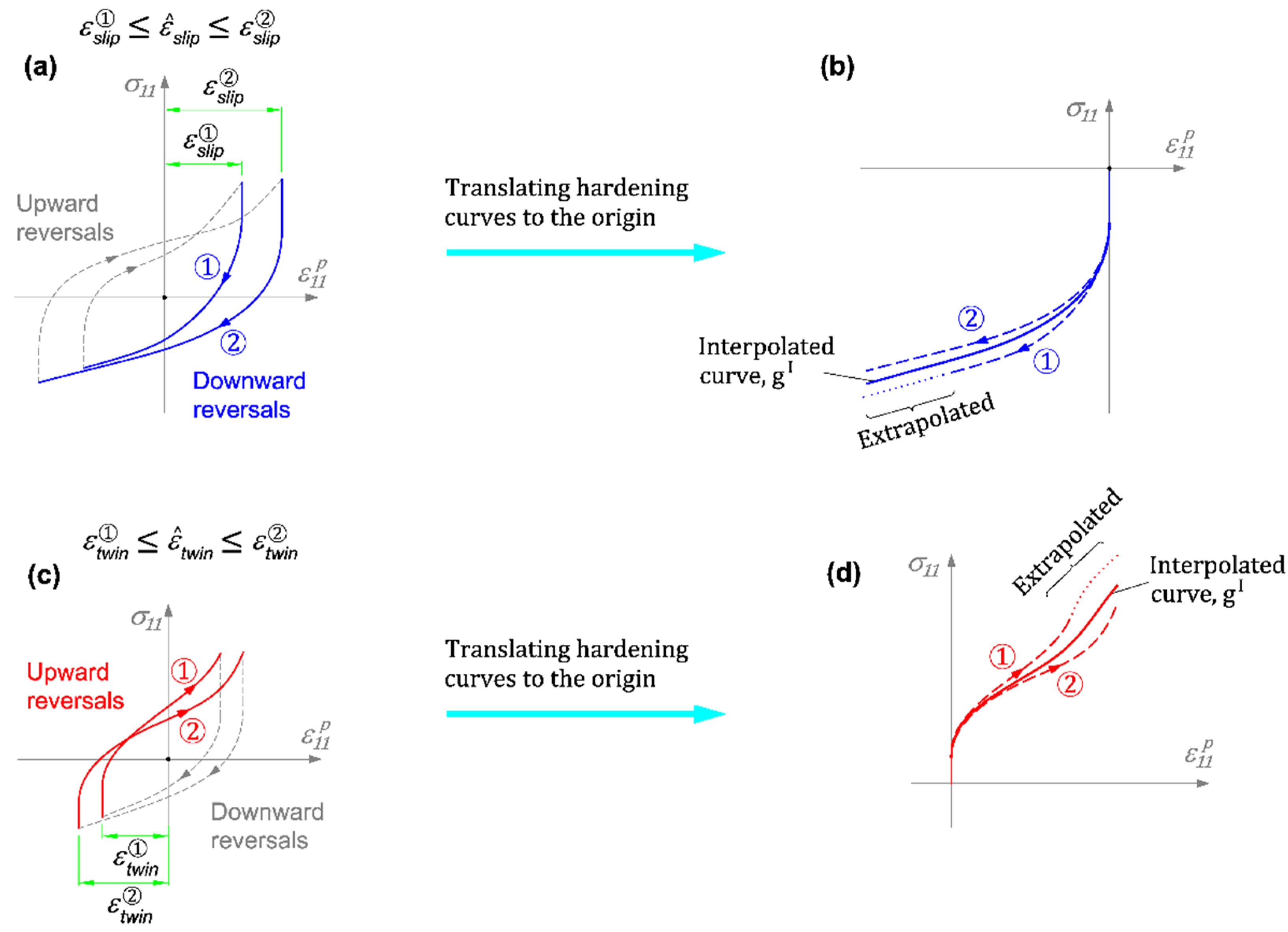
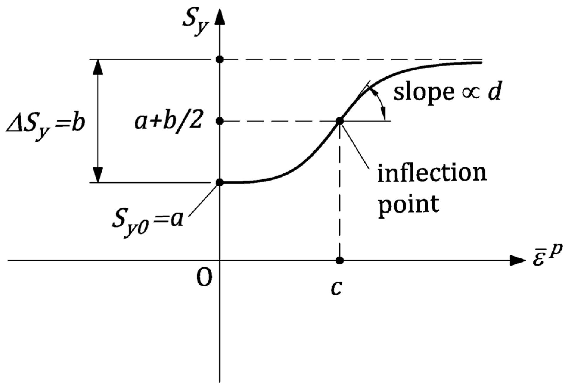
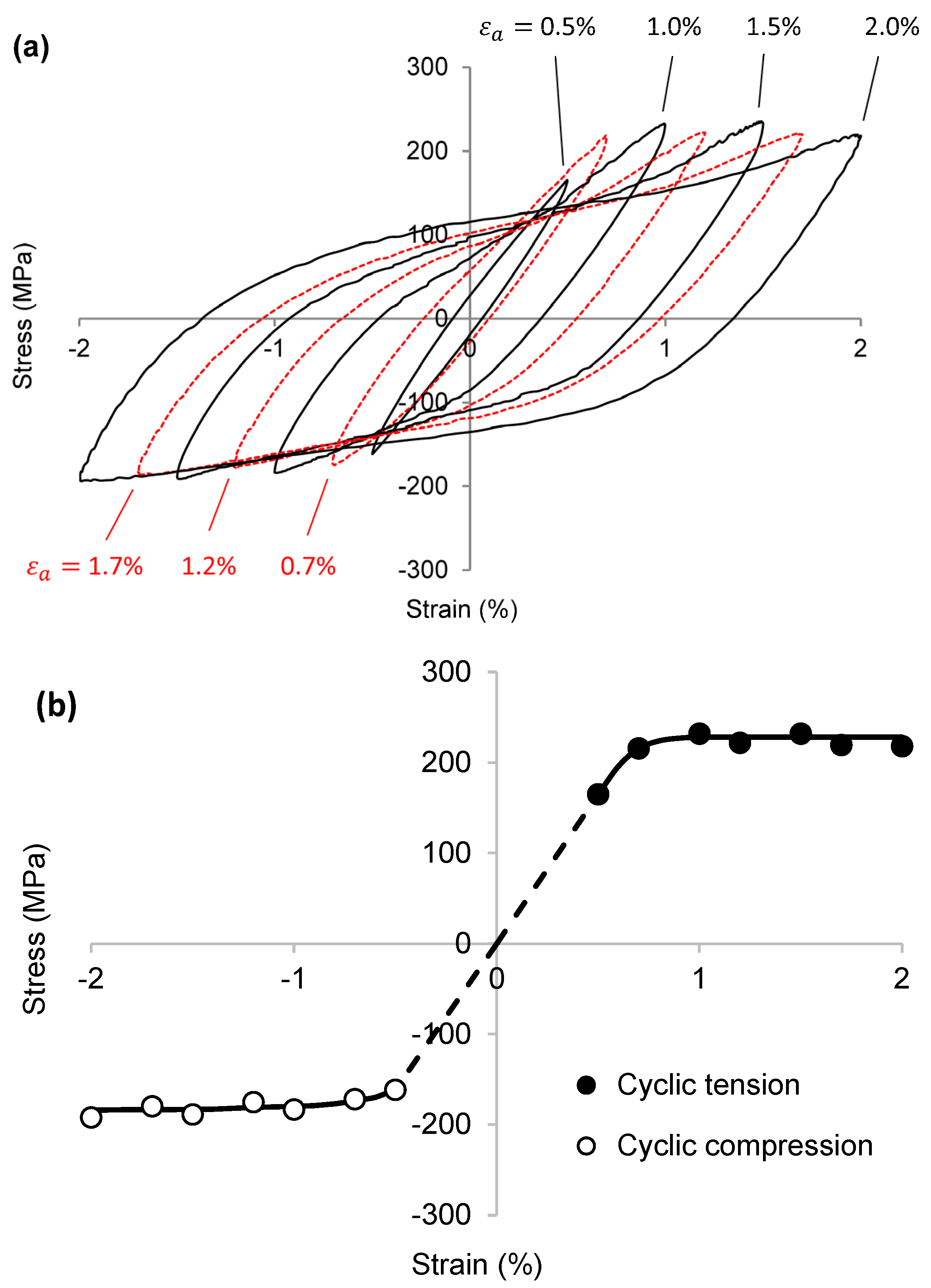
Available plasticity models, which aim to describe the hardening behavior of wrought Mg alloys under monotonic loading or single loading-unloading, have adopted different anisotropic yield criteria, including Drucker–Prager’s criterion [35,36], and CPB06 [28,32]. However, since anisotropy is less significant for cyclic behavior, cyclic plasticity models for fatigue applications utilize a symmetric von Mises yield function [39,52]. The same yield function was adopted in the proposed model.

The initial size of the yield surface is ${\kappa }_0=S_{y0}$, where $S_{y0}$ is the yield strength of the virgin material under uniaxial loading in the reference material orientation and the reference loading direction (tension/compression). In this study, and for the numerical examples provided herein, the rolling direction (RD) was selected as the reference material orientation. To account for the SD effect in wrought Mg alloys under cyclic loading, the initial size of the yield surface is proposed to be equal to or smaller than the cyclic yield strength along the loading direction, which exhibits lower yield strength. For instance, in rolled Mg alloys, where the yield strength on the cyclic compression curve is less than that on the cyclic tension curve, the reference loading direction will be uniaxial compression. Therefore, the initial size of the yield surface ${\kappa }_0=S_{y0}\le S_{y0}^C<S_{y0}^T$, where $S_{y0}^T$ and $S_{y0}^C$ are the initial tensile and initial compressive yield strengths on the cyclic stress–strain curves, as illustrated in Figure 1. Note that cyclic tension and compression curves are constructed from the stabilized hysteresis response obtained from multiple tests under different strain amplitudes.

Through this adjustment, the yield surface captures the compressive yield strength accurately but underestimates the tensile yield strength. Hence, the elastoplastic condition in the incremental solution may be triggered for stress states that are actually elastic, which results in plastic strain accumulation. To resolve this issue, the slope of the flow curve within the “virtual plastic region” was selected very close to the elastic modulus to ensure that the plastic strain remains virtually zero. This technique results in a slight increase in the computation time. This adjustment takes advantage of the simplicity of the von Mises yield criterion while capturing the SD effect.

Because Mg is a pressure-independent material [53,54], the associated flow rule was utilized in this model.

2.1.2. Flow Curves

The stabilized hysteresis loops under uniaxial cyclic loading are the inputs to the proposed constitutive model. These curves are obtained experimentally from fully reversed strain-controlled tests under a few different constant strain amplitudes. For uniaxial loading under an arbitrary strain amplitude, the cyclic flow curve for upward and downward reversals is obtained from linear interpolation between the experimentally obtained hysteresis loops. Figure 2 displays the interpolation scheme between the experimentally obtained stabilized hysteresis loops.

Figure 2a,b illustrate the interpolation between two downward reversal hardening curves associated with two stabilized hysteresis loops, where the accumulated slip strain, ${\widehat{\epsilon }}_{slip}$, is ${\epsilon }_{slip}^{①}\le {\widehat{\epsilon }}_{slip}\le {\epsilon }_{slip}^{②}$. Similarly, Figure 2c,d display the interpolation between two upward reversal hardening curves, where the residual twin strain, ${\widehat{\epsilon }}_{twin}$, is ${\epsilon }_{twin}^{①}\le {\widehat{\epsilon }}_{twin}\le {\epsilon }_{twin}^{②}$. The interpolated curves for upward and downward reversals, $g^I\left({\overline{\epsilon }}^p\right)$, are obtained from,

$$\begin{gathered} g^I\left({\overline{\epsilon }}^p\right)=w^{①}·{ g}^{①}\left({\overline{\epsilon }}^p\right)+w^{②}·g^{②}\left({\overline{\epsilon }}^p\right) \\ {w}^{①}=\frac{{\epsilon }_{slip (or twin)}^{②}-{\widehat{\epsilon }}_{slip (or twin)}}{{\epsilon }_{slip (or twin)}^{②}-{\epsilon }_{slip (or twin)}^{①}}; w^{②}=1-w^{①} \end{gathered}$$

(1)

where $g^{①}\left({\overline{\epsilon }}^p\right)$ and ${ g}^{②}\left({\overline{\epsilon }}^p\right)$ are any functions fitted to the two hardening curves, and $w^{①}$ and $w^{②}$ are the corresponding weight factors, and ${\overline{\epsilon }}^p$ is the equivalent plastic strain.

The cyclic flow curve in the current loading reversal is controlled by the history of plastic deformations in previous reversals. This phenomenon is specifically evident in the case of VAL, where twin deformation in a loading reversal may not be fully recovered in subsequent reversal. Hence, the history of the plastic deformation is recorded by calculating the accumulated slip strain and residual twin strain during the course of cyclic loading. The proposed model, being phenomenological and continuum-based, identifies the mode of plastic deformation according to the loading direction and assumes that the material has a perfect crystallographic texture. For instance, it is known that rolled Mg sheets possess a preferred crystal orientation, such that the c-axis of the HCP structure is dominantly oriented along the sheet’s normal direction [55]. Thus, in-plane tensile and compressive plastic strains are assumed to be accommodated by dislocation slip and twin deformation, respectively. As a result, the residual twin will increase during downward reversals, and decrease in upward reversals. The residual twin may not be negative, ${\widehat{\epsilon }}_{twin}\ge 0$, meaning that if the plastic deformation in the upward reversal continues after the residual twin is entirely recovered, the residual twin will remain zero and the dislocation slip will be responsible for the plastic deformation afterward, i.e., the remaining plastic strain is added to the accumulated slip. Hence, the residual twin and accumulated slip for rolled Mg sheets are updated in the current reversal $\left(i\right)$ from their accumulated history in reversal $(i-1)$,

$$\begin{array}{l}\mathrm{I}\mathrm{f} \mathrm{r}\mathrm{e}\mathrm{v}\mathrm{e}\mathrm{r}\mathrm{s}\mathrm{a}\mathrm{l} \left(i\right) is \mathrm{d}\mathrm{o}\mathrm{w}\mathrm{n}\mathrm{w}\mathrm{a}\mathrm{r}\mathrm{d}:{\widehat{\epsilon }}_{twin}^{\left(i\right)}={\widehat{\epsilon }}_{twin}^{\left(i-1\right)}+{\overline{\epsilon }}^{p \left(i\right)}; {\widehat{\epsilon }}_{slip}^{\left(i\right)}={\widehat{\epsilon }}_{slip}^{\left(i-1\right)}\\ \mathrm{I}\mathrm{f} \mathrm{r}\mathrm{e}\mathrm{v}\mathrm{e}\mathrm{r}\mathrm{s}\mathrm{a}\mathrm{l} \left(i\right) is \mathrm{u}\mathrm{p}\mathrm{w}\mathrm{a}\mathrm{r}\mathrm{d} \mathrm{a}\mathrm{n}\mathrm{d} {\widehat{\epsilon }}_{twin}^{\left(i-1\right)}\ge {\overline{\epsilon }}^{p \left(i\right)}:{\widehat{\epsilon }}_{twin}^{\left(i\right)}={\widehat{\epsilon }}_{twin}^{\left(i-1\right)}-{\overline{\epsilon }}^{p \left(i\right)}; {\widehat{\epsilon }}_{slip}^{\left(i\right)}={\widehat{\epsilon }}_{slip}^{\left(i-1\right)}\\ \mathrm{I}\mathrm{f} \mathrm{r}\mathrm{e}\mathrm{v}\mathrm{e}\mathrm{r}\mathrm{s}\mathrm{a}\mathrm{l} \left(i\right) is \mathrm{u}\mathrm{p}\mathrm{w}\mathrm{a}\mathrm{r}\mathrm{d} \mathrm{a}\mathrm{n}\mathrm{d} {\widehat{\epsilon }}_{twin}^{\left(i-1\right)}<{\overline{\epsilon }}^{p \left(i\right)}:{\widehat{\epsilon }}_{twin}^{\left(i\right)}=0;{\widehat{\epsilon }}_{slip}^{\left(i\right)}={\widehat{\epsilon }}_{slip}^{\left(i-1\right)}+{\overline{\epsilon }}^{p \left(i\right)}-{\widehat{\epsilon }}_{twin}^{\left(i-1\right)}\end{array}$$

(2)

where, the superscript $\left(i\right)$ and $\left(i-1\right)$ denote the reversal number. These internal variables are initialized in the first reversal as below,

$$\begin{array}{l}\mathrm{I}\mathrm{f} \mathrm{r}\mathrm{e}\mathrm{v}\mathrm{e}\mathrm{r}\mathrm{s}\mathrm{a}\mathrm{l} \left(1\right) is \mathrm{d}\mathrm{o}\mathrm{w}\mathrm{n}\mathrm{w}\mathrm{a}\mathrm{r}\mathrm{d}:{\widehat{\epsilon }}_{twin}^{\left(1\right)}={\overline{\epsilon }}^{p \left(1\right)}; {\widehat{\epsilon }}_{slip}^{\left(1\right)}=0\\ \mathrm{I}\mathrm{f}\mathrm{r} \mathrm{e}\mathrm{v}\mathrm{e}\mathrm{r}\mathrm{s}\mathrm{a}\mathrm{l} \left(1\right) is \mathrm{u}\mathrm{p}\mathrm{w}\mathrm{a}\mathrm{r}\mathrm{d}:{\widehat{\epsilon }}_{twin}^{\left(1\right)}=0; {\widehat{\epsilon }}_{slip}^{\left(1\right)}={\overline{\epsilon }}^{p \left(1\right)}\end{array}$$

(3)

The updated internal variables ${\widehat{\epsilon }}_{twin}$ and ${\widehat{\epsilon }}_{slip}$ along with Equation (1) are used to obtain the interpolated flow curve for the subsequent reversal $(i+1)$.

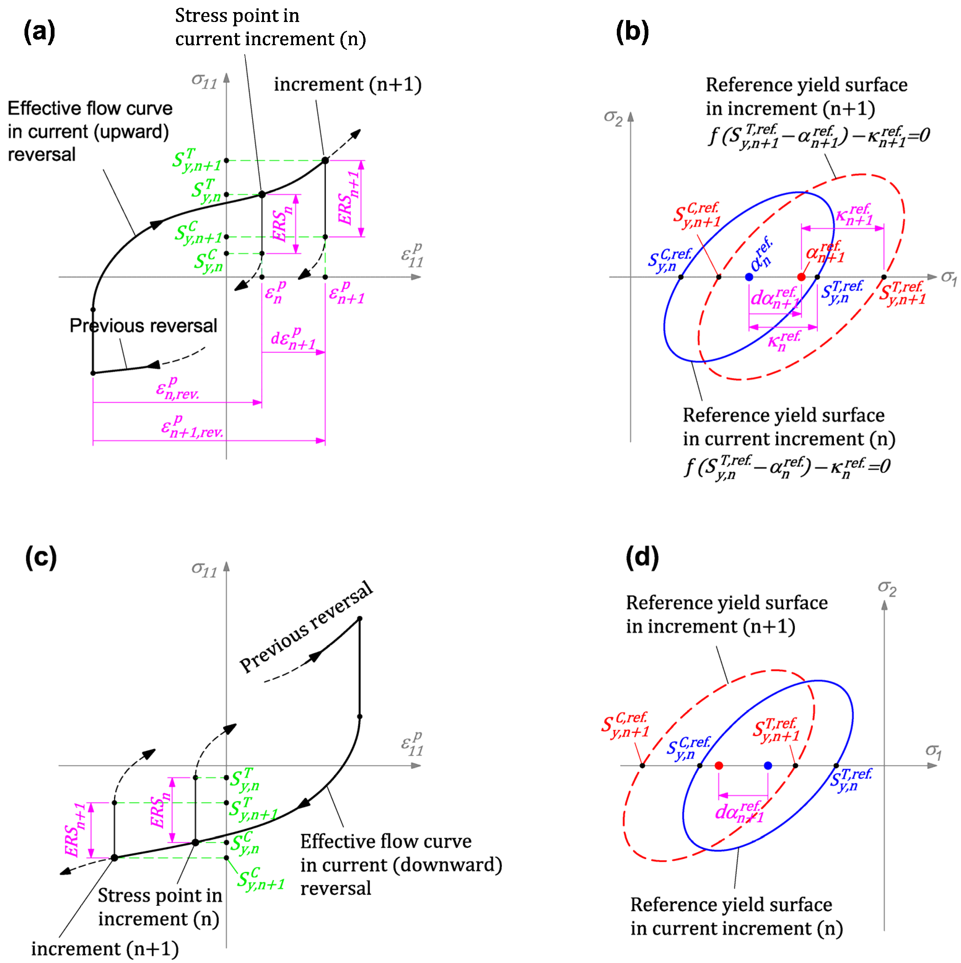
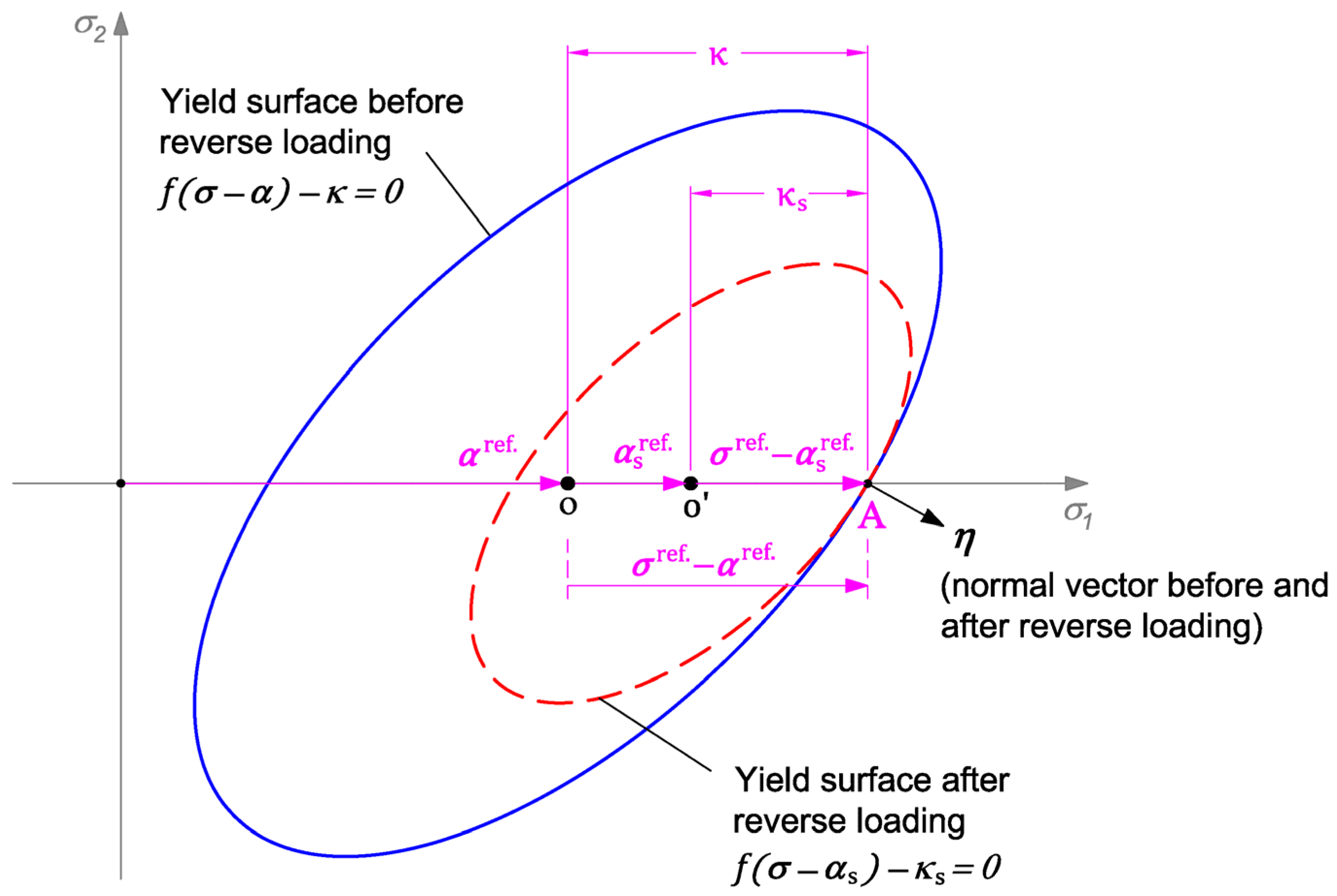
2.1.3. Hardening Rule

Plasticity models, depending on their application, may utilize different hardening rules. The models that have been developed to describe the behavior of HCP metals under monotonic loading often consider the yield function as the iso-strain yield loci [56,57,58]. These models employ an isotropic–distortional hardening rule to explain the anisotropic and/or asymmetric evolution of the yield loci. The hardening rule in these models accounts for the evolution of the size and shape of the yield function, but back stress evolution is suppressed. On the other hand, constitutive models that aim to explain loading-unloading response (such as spring-back in sheet forming applications), comprise a yield function specifying the elastic response domain of the material. These constitutive models mostly employ an isotropic–distortional hardening model [28,31,32,59], with the level of distortion in these models being more significant than that in the monotonic plasticity models. These models account for the Bauschinger effect by a severe distortion of the yield surface. The non-kinematic hardening rule imposes a constraint on the yield function to enclose the origin of the stress space over the course of plastic deformation [27,59]. This means that under uniaxial cyclic loading, the onset of plastic deformation for upward reversals must occur at a tensile (positive) stress, and for downward reversals must be at a compressive (negative) stress. However, the stabilized cyclic hysteresis behavior of wrought Mg alloys exhibits minimal elastic response, resulting in a tensile yield stress in downward reversals, and more significantly, a compressive yield stress in upward reversals [45,60,61,62]. Figure 3 depicts a typical stabilized hysteresis response of AZ31B-H24 under uniaxial cyclic loading and highlights the yield stresses in upward and downward reversals. Consequently, the non-kinematic hardening rules overestimate the domain of the elastic response of wrought Mg alloys under cyclic loading and cannot explain the early stages of post-yield behavior.

Nevertheless, non-kinematic hardening rules may reasonably describe the hardening behavior for sheet-forming applications because severe plasticity is involved and the domain of transient hardening in the early stages of post-yielding is insignificant compared to the overall plastic deformation. However, the level of plasticity in fatigue applications is substantially less than in forming, which increases the importance of the transient hardening behavior in the stabilized cyclic response. Therefore, non-kinematic hardening rules, which are not capable of describing the transient behavior, are not favorable for fatigue applications. A limited number of plasticity models have adopted combined isotropic–kinematic hardening rules to capture the hardening behavior of Mg in the first cycle [34,35,36], and the subsequent cycles [52].

To enhance the description of the transient hardening under cyclic loading, the offset to calculate the yield stress for cyclic plasticity modeling is often less than the 0.2% that is common for monotonic loading. As suggested in [64], the yield offset of 0.01% was considered in the present study.

A combined isotropic–kinematic hardening rule is proposed in this study to explain the asymmetric stabilized cyclic hardening behavior of wrought Mg alloys. Two hardening parameters are involved in this hardening model: back stress tensor, $\mathit{\alpha }$, and the size of the yield surface, $\kappa$. Hence, the yield surface is in the form of $f\left(\mathit{\sigma }-\mathit{\alpha }\right)=\kappa$. The back stress increment is governed by the stress and back stress tensors, equivalent plastic strain increment, and the history of plastic deformation, i.e., $d\mathit{\alpha }=d\mathit{\alpha }\left(\mathit{\sigma },\mathit{\alpha },{{\widehat{\epsilon }}_{slip},{\widehat{\epsilon }}_{twin},d\overline{\epsilon }}^p\right)$. The size of the yield surface is determined from the history of deformation and the equivalent plastic strain accumulated in the current reversal, $\kappa =\kappa \left({\widehat{\epsilon }}_{slip},{\widehat{\epsilon }}_{twin},{\overline{\epsilon }}_{rev.}^p\right)$. It is to be noted that in this paper, regular and bold variables denote scalar and tensor variables, respectively.

Since the focus of this research is to introduce a cyclic plasticity model under uniaxial VAL, the hardening rule proposed herein specifies the evolution of the yield surface under uniaxial tension–compression loading, called here the reference frame. The hardening parameters in the reference frame are determined from the uniaxial stabilized hysteresis loops based on the history of the deformation and the equivalent plastic strain. The extension of the proposed hardening rule to multiaxial loading is out of the scope of this research and will be introduced in a separate study.

The proposed hardening rule for the reference frame is illustrated in Figure 4. The hardening rule for an upward reversal is schematically shown in Figure 4a,b, and for a downward reversal is shown in Figure 4c,d.

Figure 4a illustrates the effective flow curve for an upward reversal, which is obtained through the interpolation procedure displayed in Figure 2. In each time increment, $n$, the stress point is found on the effective flow curve by knowing the plastic strain accumulated in the current reversal, ${\epsilon }_{n,rev.}^p$ (the subscript, $n,$ represents the increment number). This figure also shows the stress points in the current time increment, $n$, and the subsequent increment, $n+1$. For upward reversals, the tensile yield stress, $S_y^T$, at each stress point is equal to the flow stress in that time increment. The compressive yield stress, $S_y^C$, is obtained from the elastic region size ($ERS$), which is a function of the history of deformation. The ERS represents the size of the yield surface and is equal to the difference between tensile and compressive yield strengths in the reference frame, i.e., $ERS=S_y^T-S_y^C$. For instance, for the current time increment:

$$S_{y,n}^C=S_{y,n}^T-{ERS}_n\left({\widehat{\epsilon }}_{slip}\right),$$

(4)

The $ERS$ is updated in each elastoplastic time increment, as ${\widehat{\epsilon }}_{slip}$ evolves. If loading is reversed in the present increment, the effective flow curve that is obtained from interpolation between the experimental flow curves is updated. If the loading is not reversed, the current flow curve is still effective for the next increment. In either case, the stress point in the subsequent time increment, $n+1$, will be on the effective flow curve.

Figure 4b schematically illustrates the evolution of the yield surface in the reference frame for upward reversals. The hardening parameters of the reference yield surface are determined from the tensile and compressive yield stresses obtained from the effective flow curve, shown in Figure 4a.

The hardening rule for downward reversals is schematically shown in Figure 4c,d. Figure 4d illustrates the effective flow curve, and Figure 4d displays the evolution of the reference yield surface. As shown in Figure 4c, contrary to upward reversals, the compressive yield stress is located on the flow curve, and the tensile yield stress is obtained from:

$$S_{y,n}^T=S_{y,n}^C+{ERS}_n\left({\widehat{\epsilon }}_{twin}\right).$$

(5)

After determination of the tensile and compressive yield stresses in the reference frame, the hardening parameters are found from ${\alpha }_{n+1}^{ref.}=\left(S_{y,n+1}^{T,ref.}+S_{y,n+1}^{C,ref.}\right)/2$ and ${\kappa }_{n+1}^{ref.}=\left(S_{y,n+1}^{T,ref.}-S_{y,n+1}^{C,ref.}\right)/2$. It is noteworthy that these equations are valid only for symmetric yield functions, such as von Mises.

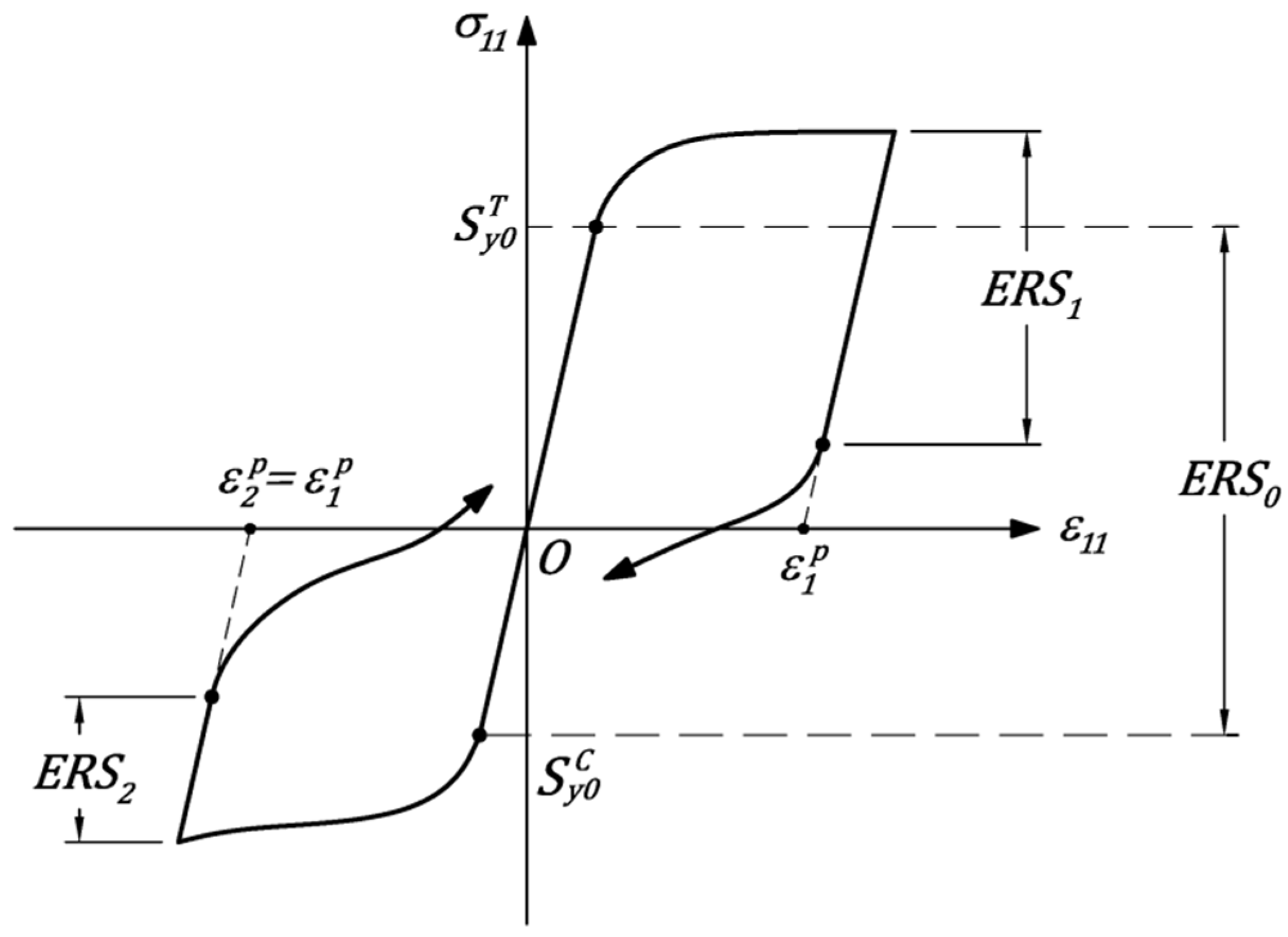
2.1.4. Modeling Cyclic Characteristics

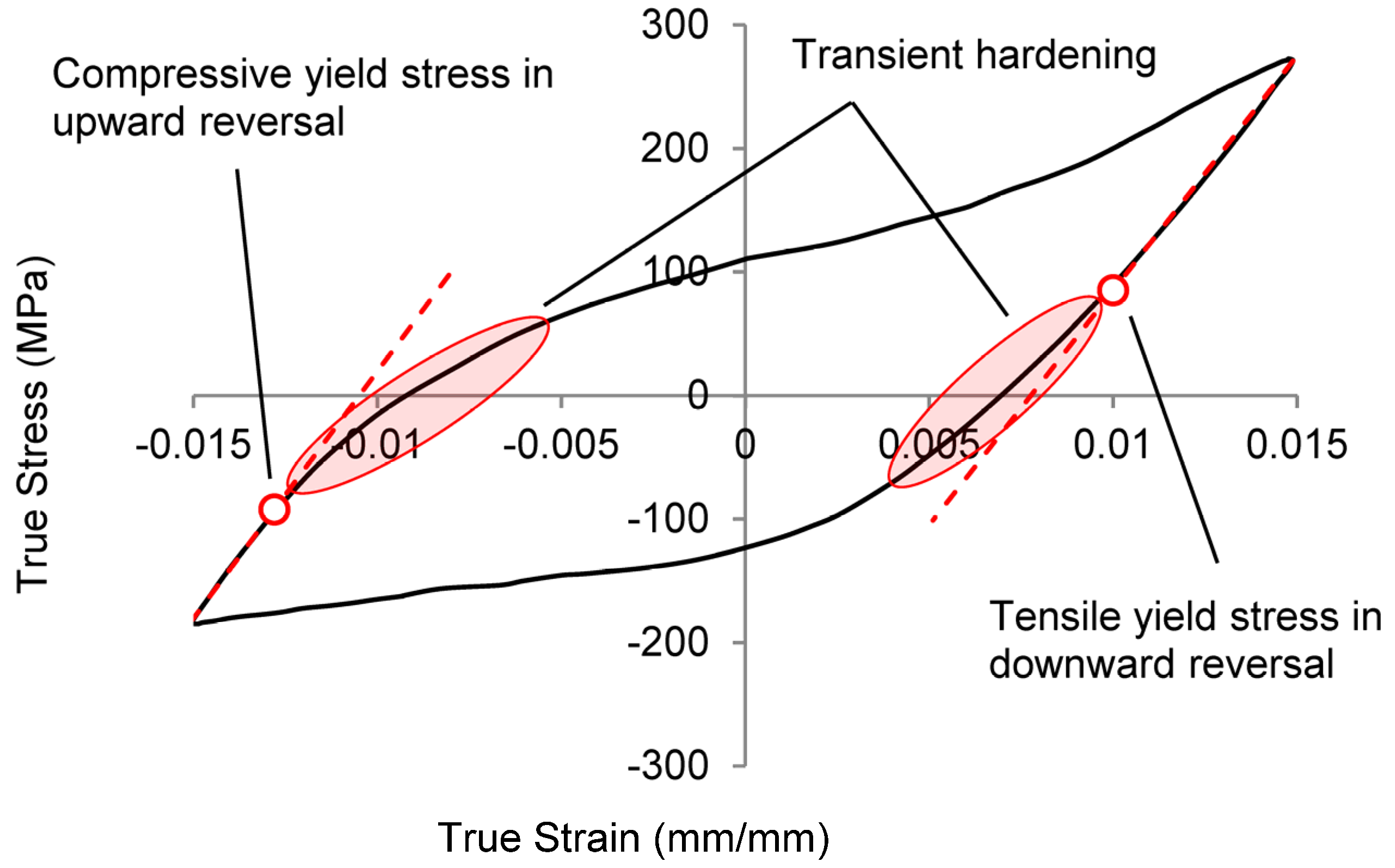
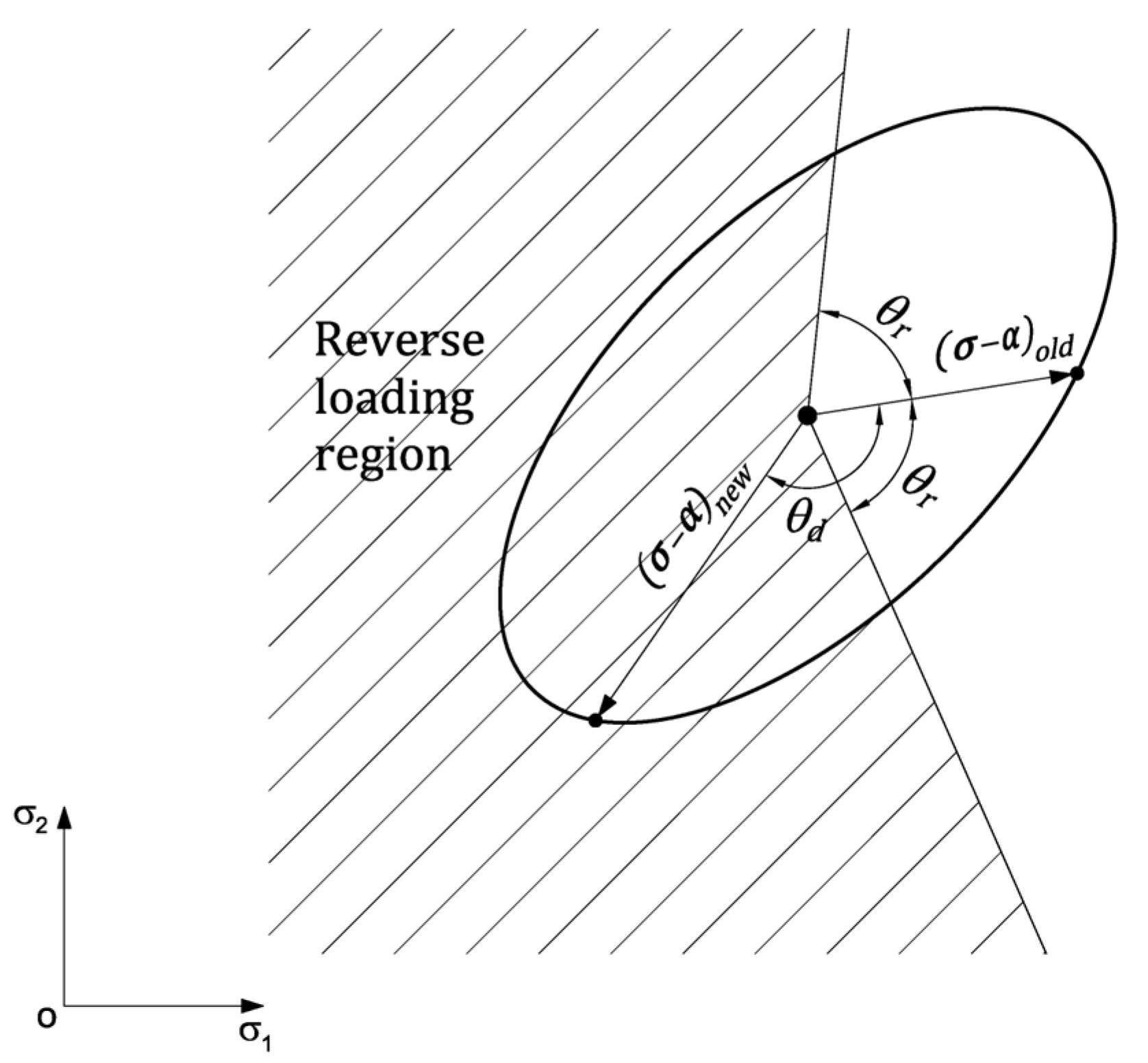
• Reversed loading and asymmetric hardening

For constitutive models aiming to explain the cyclic behavior of materials, an essential element is the reversed loading criterion. This is especially important for materials with asymmetric hardening behavior because this rule allows the model to follow the appropriate hardening curve. The criterion proposed by Lee et al. [13] was adopted in this research. According to this criterion, reverse loading occurs if the angle between two subsequent points on the yield surface, ${\theta }_d$, is greater than a predefined reference angle,${\theta }_r$. Figure 5 illustrates the reverse loading criterion on the von Mises yield function in the two-dimensional principal stress space.

The angle between two subsequent points on the yield surface, ${\theta }_d$, is obtained from

$${\theta }_d={\cos }^{-1}\left(\frac{{\left(\mathit{\sigma }-\mathit{\alpha }\right)}_{\mathit{o}\mathit{l}\mathit{d}}}{{‖\mathit{\sigma }-\mathit{\alpha }‖}_{old}}:\frac{{\left(\mathit{\sigma }-\mathit{\alpha }\right)}_{\mathit{n}\mathit{e}\mathit{w}}}{{‖\mathit{\sigma }-\mathit{\alpha }‖}_{new}}\right),$$

(6)

and the reference angle was taken to be ${\theta }_r=\pi /2$.

During the incremental solution, in the first time increment that yielding occurs, the stabilized uniaxial cyclic tension/compression curve is used as the flow curve. For subsequent elastoplastic increments, the angle ${\theta }_d$ is calculated between the current stress point and the most recent point on the yield surface using Equation (6). For ${\theta }_d<{\theta }_r$, the previous flow curves are maintained, and if ${\theta }_d>{\theta }_r$, the effective flow curve is updated according to the slip or residual twin accumulated from the onset of loading. The details of the flow curve updating procedure are explained in Section 2.1.2.

Early yielding and asymmetric hardening under cyclic loading are characteristics of wrought Mg alloys [65,66]. Early yielding on cyclic curves is partially attributed to the Bauschinger effect, i.e., plastic deformation increases the yield strength in the direction of plastic flow but decreases the yield strength in the opposite direction. In addition, different dominant deformation mechanisms (twinning vs. untwinning/slip) in the upward and downward reversals are responsible for dissimilar yield strength and hardening behavior for different reversals. Partridge [67] reported that less activation stress is required for untwinning as compared to that for twinning. This is related to nucleation, which happens in twinning but does not occur or does not easily occur in untwinning [68]. The asymmetric yield strength and hardening behavior of wrought Mg alloys under reversed loading are schematically illustrated in Figure 6. One should note that the tension and compression curves in this figure represent the cyclic curves, and the unloading curves correspond to the stabilized cyclic hysteresis response. As shown in this figure, the initial elastic region size (i.e., after the cyclic behavior is stabilized) is ${ERS}_0$. It has been reported that the elastic region size is smaller for a compression–tension load sequence than for a tension–compression sequence for AZ31B and ZK60A alloys [45,68], i.e., ${ERS}_2<{ERS}_1<{ERS}_0$. This observation shows that separate adjustments are needed for the abrupt change in the elastic region size when the material starts to deform plastically under tension or compression.

The early yielding after reversed loading is an indication of instant softening, which may be explained by an immediate change in the back stress. Figure 7 illustrates how the sudden shrinkage of the yield surface affects the back stress in the reference frame. As shown in this figure, the center of the yield surface instantly changes from o to o’ once the stress state reaches the yield surface (point A) and the reversed loading condition is satisfied at this point $\left({\theta }_d>{\theta }_r\right)$. An assumption in this model is that the yield surface maintains its shape during plastic deformation and after shrinkage.

Due to the abrupt change in the size and location of the yield surface, obtaining a converged solution requires that the yield surface after reverse loading be tangent to the previous yield surface at the current stress point, $A$. Thus, the proposed model assumes that the yield surface after shrinkage shares the same normal vector, $\mathit{\eta }$, as the yield surface before shrinkage. Therefore, the updated back stress is obtained from:

$${\mathit{\alpha }}_{\mathit{s}}^{ref.}={\mathit{\sigma }}^{ref.}-\frac{{\kappa }_s}{\kappa }\left({\mathit{\sigma }}^{ref.}-{\mathit{\alpha }}^{ref.}\right),$$

(7)

where, the subscript $s$ in ${\mathit{\alpha }}_{\mathit{s}}^{ref.}$ and ${\kappa }_s$ denotes the hardening parameters after shrinkage, i.e., reverse loading.

B.

Stabilized stress–strain response

The proposed plasticity model is intended to predict the stabilized cyclic stress–strain response. Thus, the flow curve in the first inelastic reversal under uniaxial loading is essentially the cyclic tension or compression curve. The flow curve for subsequent reversals represents the stabilized material response under cyclic loading. In the stabilized cycle, the cyclic hardening/softening behavior is saturated and the hysteresis response forms a closed loop. Consideration of the stabilized cycle and its consequences impose some constraints on the construction of the flow curves under VAL conditions.

Figure 8 illustrates the considerations proposed in this research to generate the stabilized material response under VAL. Figure 8a displays an arbitrary VAL spectrum as the input load to the material. The VAL spectrum is modified by adding the envelope cycle to the beginning of the spectrum. Figure 8b depicts the modified spectrum with two reversals added after the first reversal (E1 and E2) to represent the envelope cycle. This step assures that the accumulated slip and residual twin are found properly for the stabilized cycles from the onset of loading. In other words, disregarding this step may result in an incorrect calculation of the deformation history and the flow curve in the first VAL block of cycles. The reason is that at the onset of the first loading block, the material is in the virgin state with no plastic strain history. Hence, the accumulated plastic deformation calculated in the first block does not represent that in subsequent blocks, where some accumulated slip and/or twin deformations exist in the material from the beginning of the block. Because the slip and twin calculations are not reliable for the first (envelope) cycle, the flow curve for this cycle is constructed according to the strain range of the envelope cycle, i.e., the flow curves are obtained from the constant amplitude hysteresis loops, which are the inputs to the model. Furthermore, knowing that the stabilized stress–strain response forms a closed hysteresis loop, the flow curve for each reversal (after the second reversal) is found such that it closes the most recent open reversal. For instance, in the loading spectrum shown in Figure 8, (extension of) the flow curves for reversals ③ and ⑤ are required to close the reversal ②, i.e., to pass through the point where the reversal ② started from, see Figure 8c. The other point to consider is that after an open reversal is closed by the current reversal and the loading continues, the flow curve is governed by the next recent open reversal in the same loading direction (upward/downward reversal). As displayed in Figure 8c, after reversal ④ closes the most recent open reversal, i.e., reversal ③, the flow curve for the continuation of reversal ④ is dictated by reversal ②.

The following rules are followed for constructing the flow curves under variable amplitude loading:

• Following the standard practice of cycle counting in VAL, rearrange the VAL block such that the second and the third reversals constitute the envelope cycle of the loading block.
• Use the cyclic tension/compression curve as the flow curve for the first reversal.
• For the second and the third reversals, i.e., the envelope cycle, the flow curve is determined according to the strain range for this cycle (through linear regression between the input constant amplitude stabilized hysteresis loops).
• The flow curves for the subsequent upward and downward reversals are obtained according to the residual twin and accumulated slip, respectively.
• If the current reversal closes the most recent open reversal and continues, the flow curve for the next recent open reversal in the same direction as the current reversal is followed.

2.2. Numerical Implementation

The numerical algorithm proposed by Lee et al. [13] was modified and adopted in this study. The numerical formulation was implemented into a UMAT subroutine that runs with the Abaqus/Standard 2019 finite element package [69].

The numerical formulation aims at obtaining the unknown variables in the current increment, $n$, using the known variables from the previous increment, $n-1$. The known variables at the beginning of each increment are the total strain increment for the current time increment, as well as the stress and strain tensors and the state variables from the previous time increment. State variables include but are not limited to elastic and plastic strain tensors, and the back stress tensor. The unknown variables are elastic and plastic strain tensors and the stress and back stress tensors in the current increment. All the variables are related to the equivalent plastic strain increment as well as the deformation history. The equivalent plastic strain increment and the related variables are found in each increment through an iterative process. At the end of each iteration, the convergence of the solution is examined using the consistency condition. The procedure for updating the variables in each iteration is explained below.

The consistency condition in continuum plasticity requires that the stress point remains on the yield surface throughout plastic deformation, which means that:

$$\phi =f\left(\mathit{\sigma }-\mathit{\alpha }\right)-\kappa =0,$$

(8)

Assuming that the current increment is fully elastic, the elastic trial stress is calculated for the given total strain increment, $∆{\mathit{\epsilon }}_n$, while the other variables remain unchanged:

$${\mathit{\sigma }}_n^{Tr}={\mathit{\sigma }}_{n-1}+{\mathit{C}}^{\mathit{e}}·∆{\mathit{\epsilon }}_n; {\mathit{\alpha }}_n^{Tr}={\mathit{\alpha }}_{n-1}; {\overline{\epsilon }}_{rev.,n}^{p,Tr}={\overline{\epsilon }}_{rev.,n-1}^p,$$

(9)

in which the superscript $Tr$ denotes the trial state, and ${\mathit{C}}^e$ is the known elastic stiffness tensor. The subscript $rev.$ denotes that the corresponding variable is related to the current reversal and resets after each reversal. The assumption of an elastic increment is then evaluated against the consistency condition for the yield surface:

$${\phi }_n^{Tr}=f\left({\mathit{\sigma }}_n^{Tr}-{\mathit{\alpha }}_n^{Tr}\right)-{\kappa }_n\left({\widehat{\epsilon }}_{slip},{\widehat{\epsilon }}_{twin},{\overline{\epsilon }}_{rev.,n}^{p,Tr}\right).$$

(10)

For ${\phi }_n^{Tr}\le 0$, the stress state is inside or on the yield surface, and the elastic solution is valid. Hence, the true values of the variables for the current increment are equal to the trial values. Otherwise, for ${\phi }_n^{Tr}>0$, the stress state is located outside the yield surface and the stress tensor and the hardening parameters are updated to satisfy $\phi =0$. Therefore, the elastic trial values are corrected through an iterative procedure in the elastoplastic solution. The elastoplastic solution is initialized by:

$$k=1; {\mathit{\sigma }}_n^{\left(k\right)}={\mathit{\sigma }}_n^{Tr}; {\mathit{\alpha }}_n^{\left(k\right)}={\mathit{\alpha }}_n^{Tr}; ∆{\overline{\epsilon }}_n^{p\left(k\right)}=∆{\overline{\epsilon }}_0^p; {\overline{\epsilon }}_n^{p\left(k\right)}={\overline{\epsilon }}_{rev.,n-1}^p+∆{\overline{\epsilon }}_n^{p\left(k\right)},$$

(11)

where the superscript $k$ stands for the iteration number, and $∆{\overline{\epsilon }}_0^p$ is an arbitrary initial value for the equivalent plastic strain increment. Flow direction, $\mathit{\eta }$, according to the associated flow rule is normal to the yield surface at the current stress point,

$$\mathit{\eta }={\left.\frac{\partial f(\mathit{\sigma }-\mathit{\alpha })}{\partial (\mathit{\sigma }-\mathit{\alpha })}\right|}_{{\mathit{\sigma }}_n^{\left(k\right)}-{\mathit{\alpha }}_n^{\left(k\right)}},$$

(12)

and the plastic strain increment tensor and the Cauchy stress tensor are updated

$${∆\mathit{\epsilon }}_n^{p\left(k\right)}=∆{\overline{\epsilon }}_n^{p\left(k\right)}\mathit{\eta },$$

(13)

$$\begin{gathered} {\mathit{\sigma }}_n^{\left(k\right)}={\mathit{\sigma }}_{n-1}+{\mathit{C}}^{\mathit{e}}:∆{\mathit{\epsilon }}_n^{e\left(k\right)}={\mathit{\sigma }}_{n-1}+{\mathit{C}}^{\mathit{e}}:\left(∆{\mathit{\epsilon }}_n-∆{\mathit{\epsilon }}_n^{p\left(k\right)}\right) \\ {=\mathit{\sigma }}_n^{Tr}-{\mathit{C}}^{\mathit{e}}:{∆\mathit{\epsilon }}_n^{p\left(k\right)}={\mathit{\sigma }}_n^{Tr}-∆{\overline{\epsilon }}_n^{p\left(k\right)}{\mathit{C}}^{\mathit{e}}:{\left.\frac{\partial f(\mathit{\sigma }-\mathit{\alpha })}{\partial (\mathit{\sigma }-\mathit{\alpha })}\right|}_{{\mathit{\sigma }}_n^{(k-1)}-{\mathit{\alpha }}_n^{(k-1)}} \end{gathered}$$

(14)

The reverse loading criterion is evaluated: if ${\theta }_d>{\theta }_r$, reverse loading happens and the flow curves are updated according to the deformation history in previous reversals (${\widehat{\epsilon }}_{slip},{\widehat{\epsilon }}_{twin}$), as illustrated in Figure 2. Otherwise, the same loading reversal is still in effect and the flow curves remain the same as the previous increment. According to Figure 4, the yield stresses in the forward and (virtual) reversed loading directions ($S_{y,n}^{T\left(k\right)}$, $S_{y,n}^{C\left(k\right)}$) are obtained, and the hardening parameters in the reference frame are determined:

$${\kappa }_n^{\left(k\right)}=\left(S_{y,n}^{T\left(k\right)}-S_{y,n}^{C\left(k\right)}\right)/2, {\alpha }_n^{\left(k\right)}=\left(S_{y,n}^{T\left(k\right)}+S_{y,n}^{C\left(k\right)}\right)/2$$

(15)

The consistency condition is examined in each iteration, after updating the stress tensor and the hardening parameters,

$${\phi }_n^{\left(k\right)}=f\left({\mathit{\sigma }}_n^{\left(k\right)}-{\mathit{\alpha }}_n^{\left(k\right)}\right)-{\kappa }_n^{\left(k\right)}=0,$$

(16)

where, ${\mathit{\alpha }}_n^{\left(k\right)}=\left[{\alpha }_n^{\left(k\right)} 0 0 0 0 0\right]$ for the case of uniaxial loading along the 11 direction. The residual value obtained, $\left|{\phi }_n^{\left(k\right)}\right|$, represents the distance between the current stress state and the yield surface, which is compared with the predefined acceptable tolerance. The tolerance of $Tol={10}^{-6}$ was considered in the current work. If $\left|{\phi }_n^{\left(k\right)}\right|<Tol$ the consistency condition is satisfied, i.e., the stress state is close enough to the yield surface. Thus, variables obtained in the $k$’th iteration are accepted as the elastoplastic results for the current increment. Otherwise, the solution has to continue until the stress state converges to the yield surface. The Newton–Raphson method was used to update the equivalent plastic strain increment within the iterative solution.

Finally, the elastoplastic stiffness tensor, ${\mathit{C}}^{\mathit{e}\mathit{p}}$, is updated according to [58] with an adjustment due to the isotropic behavior assumption in the present study:

$${\mathit{C}}^{\mathit{e}\mathit{p}}=\left\{\begin{array}{ll}{\mathit{C}}^{\mathit{e}}& \mathrm{i}\mathrm{f} \mathsf{\Delta }{\overline{\epsilon }}^p=0\\ {\mathit{C}}^{\mathit{e}}-\frac{{\mathit{C}}^{\mathit{e}}:\mathit{\eta }⨂{\mathit{C}}^{\mathit{e}}:\mathit{\eta }}{\mathit{\eta }:{\mathit{C}}^{\mathit{e}}:\mathit{\eta }+h}& \mathrm{i}\mathrm{f} \mathsf{\Delta }{\overline{\epsilon }}^p>0\end{array}\right.,$$

(17)

where $h=\mathsf{\Delta }{S}_y\left({\overline{\epsilon }}^p\right)/\mathsf{\Delta }{\overline{\epsilon }}^p$ is the plastic modulus obtained from the flow curve.

3. Numerical Examples and Model Calibration

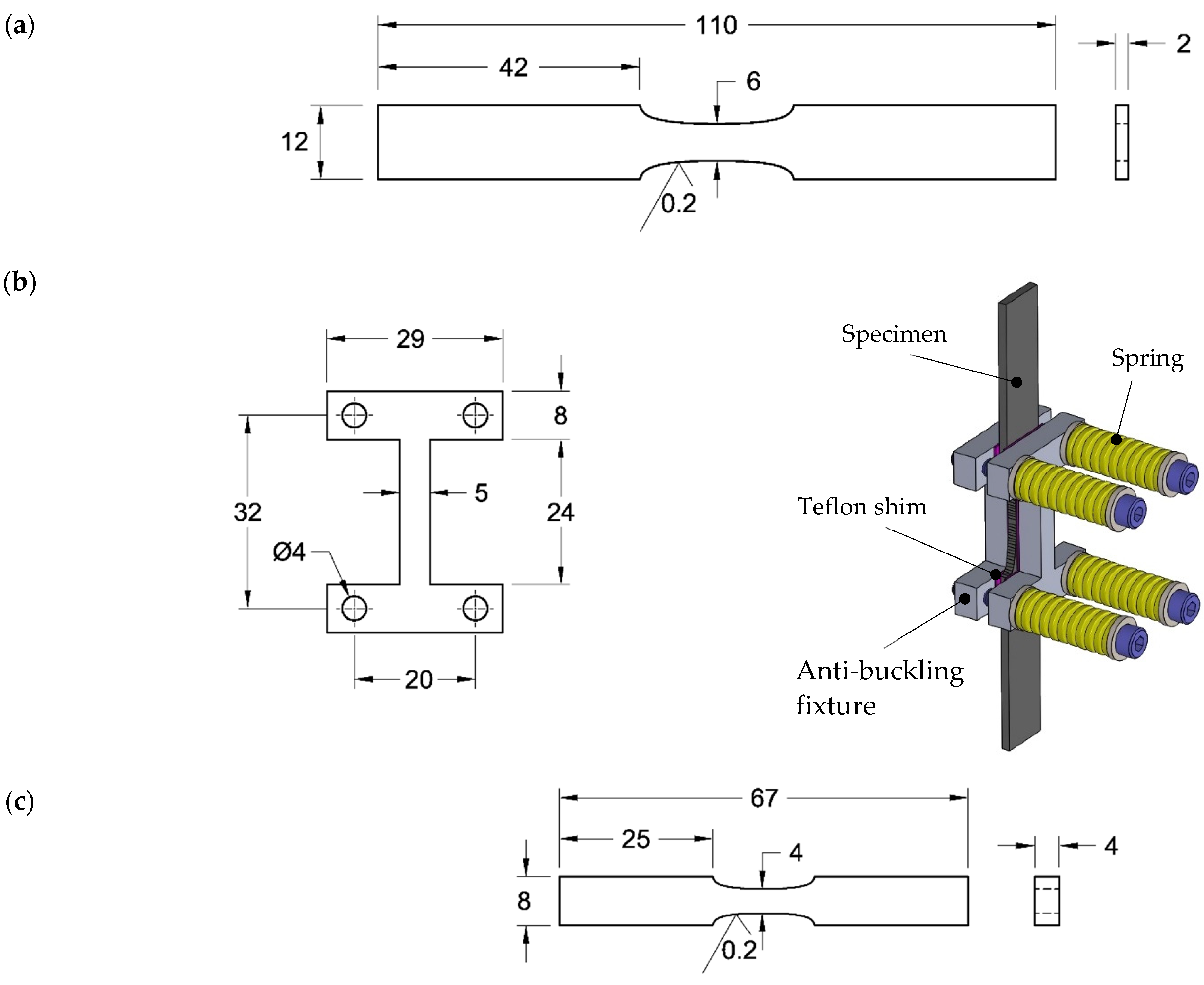
3.1. Materials and Experiments

The materials investigated in this research are ZEK100 rolled Mg sheet in 2 mm thickness, and AZ31B-H24 rolled Mg sheet in 4 mm thickness. The chemical composition is shown in

Table 1. Chemical composition of ZEK100 and AZ31B-H24 Mg alloy (in weight %).

Alloy	Zn	Al	Mn	Zr	Nd	Mg
ZEK100 [70]	1.37	0.003	0.005	0.48	0.19	Bal.
AZ31B-H24 [71]	0.915	2.73	0.375	-	-	Bal.

.

Uniaxial tension–compression fatigue testing on ZEK100 was performed using the specimen geometry shown in Figure 9a. An anti-buckling fixture, as displayed in Figure 9b, was utilized to prevent buckling in ZEK100 specimens. As depicted, Teflon shims were used on both sides between the specimen and the fixture, to minimize friction. Four springs were utilized to provide lateral support and to allow for bulging of the specimen under compressive load. Fatigue testing on AZ31B was performed on sub-size specimens with the geometry shown in Figure 9c, which enabled fatigue testing without an anti-buckling fixture. The specimens were all machined along the RD.

Engineering strain was measured using an Epsilon axial extensometer with a 6.0 mm gauge length and ±0.8 mm travel. Fatigue tests were run in strain-control mode under constant or variable amplitude loading. The constant amplitude fatigue tests were performed with strain amplitudes of ${\epsilon }_a$ = 0.2–2% and loading frequency of 0.1–0.15 Hz.

3.2. Application to Rolled ZEK100

The constitutive model proposed in this research intends to simulate the stabilized behavior of asymmetric materials under uniaxial cyclic loading. Thus, the inputs to the model include stabilized cyclic stress–strain curves and a few stabilized hysteresis loops under different strain amplitudes. Nevertheless, the model may be utilized to explain the monotonic behavior by replacing the stabilized cyclic curves with quasi-static hardening curves.

The sigmoid function below was adopted to model the stabilized cyclic tension and cyclic compression flow curves:

$$S_y=a+\frac{b}{1+{\left(c/{\overline{\epsilon }}_p\right)}^{-d}} ,$$

(18)

in which the parameters $a$, $b$, $c$, and $d$ are material constants. Figure 10 illustrates the sigmoid function and identifies the parameters for a schematic flow curve.

The double sigmoid function below was employed to explain the flow curves of the upward and downward reversals of the stabilized hysteresis loops. The flow curves for the downward and upward reversals are schematically illustrated in Figure 2b,d, respectively.

$$S_y=a+\frac{b_1}{\left[1+{\left(\frac{c_1}{{\overline{\epsilon }}_p}\right)}^{{-d}_1}\right]}+\frac{b_2}{\left[1+{\left(\frac{c_2}{{\overline{\epsilon }}_p}\right)}^{{-d}_2}\right]}$$

(19)

Figure 11a displays the half-life stabilized hysteresis loops under constant amplitude cyclic loading with the strain amplitude ranging from ${\epsilon }_a$ = 0.5–2.0%, and Figure 11b shows the uniaxial cyclic tension and compression curves, which are essentially constructed from the peak and valley points of the half-life hysteresis loops.

The material constants in Equation (18) were determined through regression using uniaxial cyclic tension and compression curves, Figure 11b.

Table 2. Material constants for stabilized cyclic tension and cyclic compression curves for ZEK100.

	$a$ (MPa)	$b$ (MPa)	$c$	$d$
Cyclic tension	100	140	0.0007	0.8
Cyclic compression	100	119	0.0010	0.4

summarizes these parameters for the stabilized cyclic curves of ZEK100.

As mentioned earlier, the proposed model describes the asymmetric initial yield strengths of wrought Mg alloys using the symmetric von Mises yield function, by assuming that ${\kappa }_0=S_{y0}<S_{y0}^C<S_{y0}^T$. As shown in Figure 10 and Table 2, the initial yield strength under both tension and compression is assumed ${\kappa }_0=S_{y0}=a$= 100 MPa, which is less than the yield strengths for both cyclic tension and cyclic compression, Figure 11b.

Four stabilized hysteresis loops with strain amplitudes of ${\epsilon }_a$ = 0.5%, 1.0%, 1.5%, and 2.0% were utilized for model calibration. The material constants in Equation (19) were determined for the upward and downward reversals of these hysteresis loops. It should be noted that the constants in Equations (18) and (19) are obtained from ${\sigma }_{11}$ vs. ${\epsilon }_{11}$ for uniaxial cyclic tension curve and upward reversals, but are calculated from $-{\sigma }_{11}$ vs. $-{\epsilon }_{11}$ for cyclic compression curve and downward reversals. The constants for upward and downward reversals of ZEK100 are listed in

Table 3. Material constants for upward and downward reversals of selected stabilized hysteresis loops for ZEK100.

	Upward Reversals
${\epsilon }_a$	${\widehat{\epsilon }}_{twin}$	$a^U$ (MPa)	$b_1^U$ (MPa)	$c_1^U$	$d_1^U$	$b_2^U$ (MPa)	$c_2^U$	$d_2^U$
0.5%	0.0024	88	500	0.0042	1.1	221	0.0500	0.3
1.0%	0.0103	113	500	0.0141	0.7	109	0.0087	7.2
1.5%	0.0202	121	297	0.0068	0.8	274	0.0227	5.0
2.0%	0.0305	86	339	0.0052	0.7	91	0.0282	9.4
	Downward reversals
${\epsilon }_a$	${\widehat{\epsilon }}_{slip}$	$a^D$ (MPa)	$b_1^D$ (MPa)	$c_1^D$	$d_1^D$	$b_2^D$ (MPa)	$c_2^D$	$d_2^D$
0.5%	0.0009	73	500	0.0083	1.4	500	0.0052	0.7
1.0%	0.0050	128	300	0.0017	1.1	300	0.0176	4.3
1.5%	0.0098	144	206	0.0011	1.3	200	0.0244	2.2
2.0%	0.0147	64	314	0.0015	1.1	200	0.0500	2.3

. These parameters are employed to construct the effective flow curve for upward and downward reversals under a given loading scenario, according to the procedure explained in Section 2.1.2.

During the numerical solution, the $ERS$ is updated in each time increment to find the size of the yield surface. The $ERS$ for a time increment is found by assuming that the loading is reversed at the end of the current time increment. Then, if the current reversal is upward, the $ERS$ is equal to the yield stress in the next (downward) reversal, ${ERS}^U=a^D$, and if the current reversal is downward, ${ERS}^D=a^U$.

After calibration of the model for ZEK100, the model predictions for the stabilized hysteresis response were compared to the experimental results. The cyclic plasticity constitutive model introduced in the previous section was implemented into a UMAT subroutine to run with Abaqus/standard. A simple FE model was generated to validate the formulation and implementation of the plasticity model. The FE model included a single eight-node linear brick element. Appropriate boundary conditions were applied to the element to ensure consistency with the experiments, i.e., a uniform stress–strain distribution. Since the model was calibrated using the stabilized behavior of the material, it is required to simulate only three reversals to obtain the stabilized hysteresis response under constant amplitude loading. Figure 12 displays the results for the four fatigue tests that were used for the model calibration and confirms that the implementation of the constitutive model and the parameter extraction were conducted successfully.

The graphs in this figure demonstrate that the material model implemented in the UMAT is well-calibrated and follows the stabilized cyclic behavior very well under different strain amplitudes. Adopting the sub-sized yield surface enabled the model to capture the smooth transition from the elastic to the elastic-plastic domain of the cyclic response on both the upward and downward reversals. In addition, as displayed in Figure 12, the hardening behavior in the downward reversals as well as the sigmoid shape of the upward reversals are well reproduced after various pre-strains in the first and second reversals. Moreover, the size of the elastic response region at the onset of upward and downward reversals is in very good agreement with the experiments, verifying that the combined isotropic–kinematic hardening rule and the abrupt shrinkage of the yield surface were successful in accounting for the asymmetric Bauschinger effect. The slight difference in hardening curves between the model and the experiments is partially due to the approximations inherent in model calibrations. The other factor contributing to the slight deviation is enforcing the conditions explained in Section 2.1.4, which are required to satisfy the essential features of a stabilized cyclic response.

3.3. Application to Rolled AZ31B

Figure 13a depicts the stabilized hysteresis response for AZ31B samples obtained under constant amplitude tests with strain amplitudes in the range of ${\epsilon }_a$ = 0.2–2.0%. Figure 13b displays the cyclic tension and cyclic compression curves. Similar to the static behavior [68], the cyclic yield strength under tension is significantly higher than that under compression for rolled AZ31B. This behavior has been reported in earlier studies [49,51].

Table 4. Material constants for stabilized cyclic tension and cyclic compression curves for AZ31B.

	$a$ (MPa)	$b$ (MPa)	$c$	$d$
Cyclic tension	127	141	0.0010	2.5
Cyclic compression	127	198	0.1000	0.4

presents the parameters of the sigmoid function given in Equation (18) for the cyclic tension and compression curves.

According to Figure 13, the yield strengths for cyclic tension and cyclic compression curves are $S_{y0}^T$ = 245 MPa and $S_{y0}^C$ = 162 MPa, respectively. However, as shown in Table 4, the initial yield strength under both tension and compression is assumed ${\kappa }_0=a$= 127 MPa, to satisfy the symmetric yield strength required by the von Mises yield function, and to enable describing the non-linear cyclic response in the small plastic strain domain.

The four hysteresis loops selected for calibration of the model for AZ31B correspond to fatigue tests with strain amplitudes of 0.5%, 0.9%, 1.2%, and 2.0%. Two sets of parameters were determined for the upward and downward reversals, which are summarized in

Table 5. Material constants for upward and downward reversals of selected stabilized hysteresis loops for AZ31B.

	Upward Reversals
${\epsilon }_a$	${\widehat{\epsilon }}_{twin,2}$	$a^U$ (MPa)	$b_1^U$ (MPa)	$c_1^U$	$d_1^U$	$b_2^U$ (MPa)	$c_2^U$	$d_2^U$
0.5%	0.0021	132	236	0.0010	1.0	122	0.0026	2.3
0.9%	0.0078	53	295	0.0013	1.0	158	0.0058	5.1
1.2%	0.0135	52	307	0.0020	0.9	152	0.0110	9.1
2.0%	0.0295	30	379	0.0025	0.8	114	0.0256	10.0
	Downward reversals
${\epsilon }_a$	${\widehat{\epsilon }}_{slip}$	$a^D$ (MPa)	$b_1^D$ (MPa)	$c_1^D$	$d_1^D$	$b_2^D$ (MPa)	$c_2^D$	$d_2^D$
0.5%	0.0008	47	272	0.0013	1.2	320	0.0500	0.5
0.9%	0.0030	15	426	0.0020	1.1	300	0.0500	0.6
1.2%	0.0058	44	318	0.0012	1.3	300	0.0500	0.6
2.0%	0.0138	47	272	0.0013	1.2	320	0.0500	0.5

.

Figure 14 compares the model predictions with the experimental results for the four constant amplitude tests that were used to extract the model parameters. Good matching of the results confirms the correct calibration of the model.

4. Model Verification

The proposed cyclic plasticity model was verified by comparing the simulation results with experimental behavior under constant amplitude loading with non-zero mean strain, and variable amplitude loading.

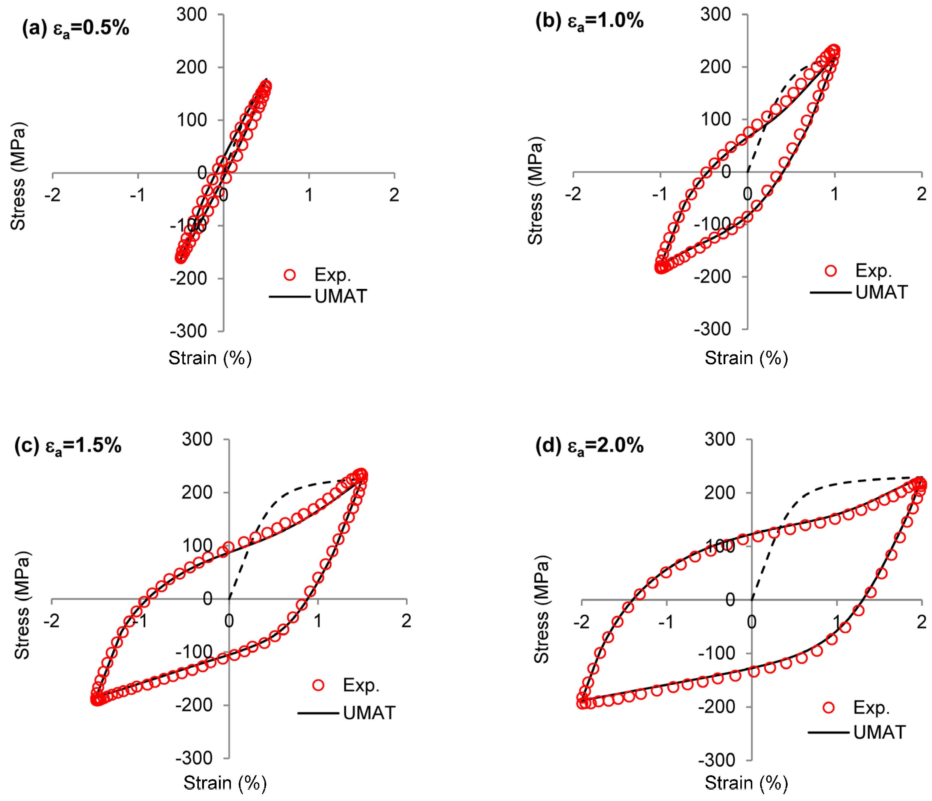
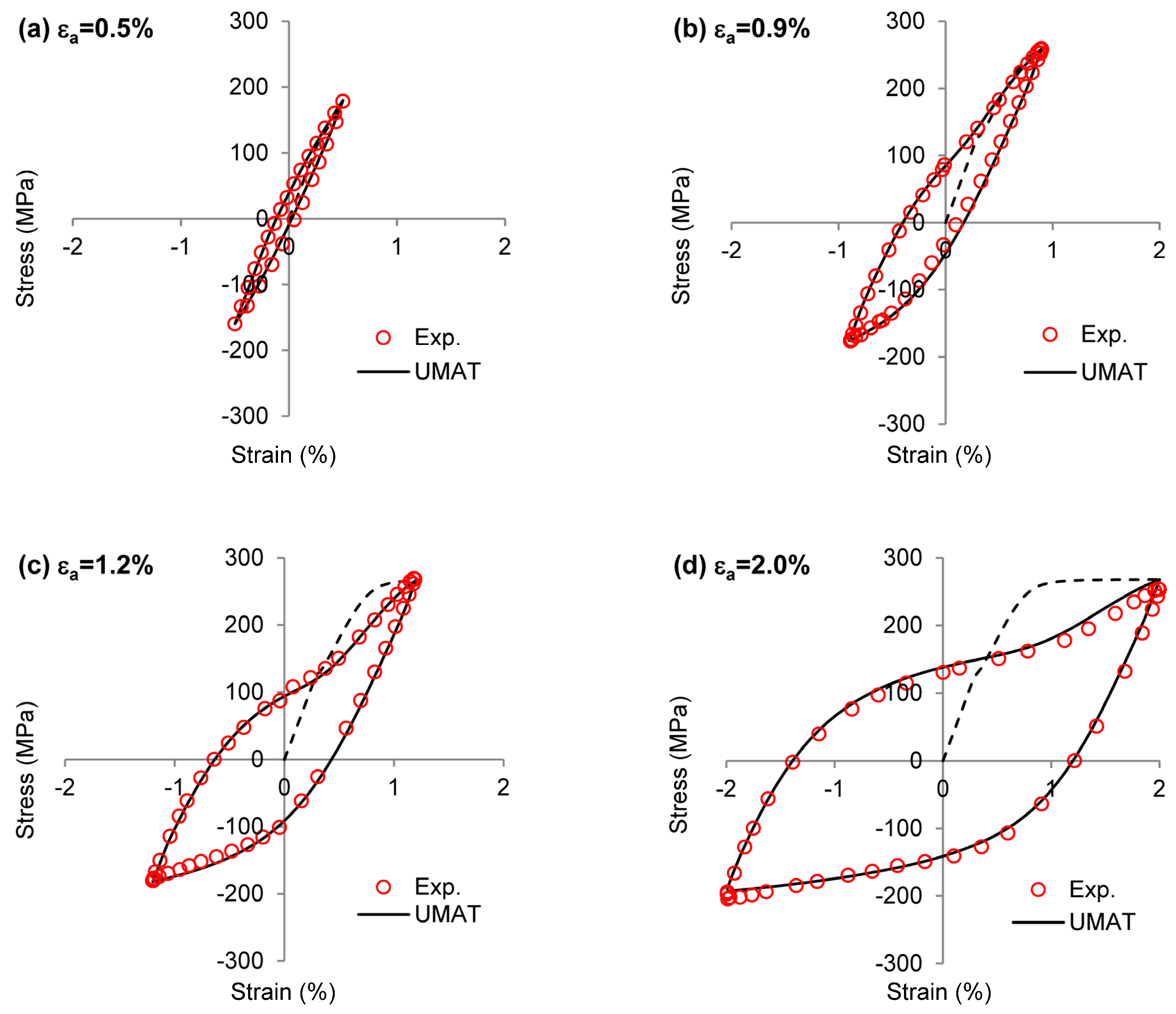
4.1. Constant Amplitude Loading

Figure 15 compares the experimental and simulation results for ZEK100 under various cyclic loading conditions.

These graphs verify that the proposed constitutive model is capable of predicting the cyclic response of the materials under constant amplitude loading. In particular, the hardening curves for downward and upward reversals were successfully predicted, which verifies that the hardening curves (i.e., the envelope cycle under VAL) are controlled by the strain range. This indicates that the interpolation schemes for the hardening parameters and the $ERS$ were effective. These verifications further confirm that the virtual size reduction in the symmetric von Mises yield surface is appropriate for modeling the asymmetric yield and hardening behavior. These graphs display close agreement between the experimental and simulation results for both the TCT and CTC load sequences, which confirms that the effect of both slip and twin pre-strain on the flow curve of the stabilized cycle is well explained.

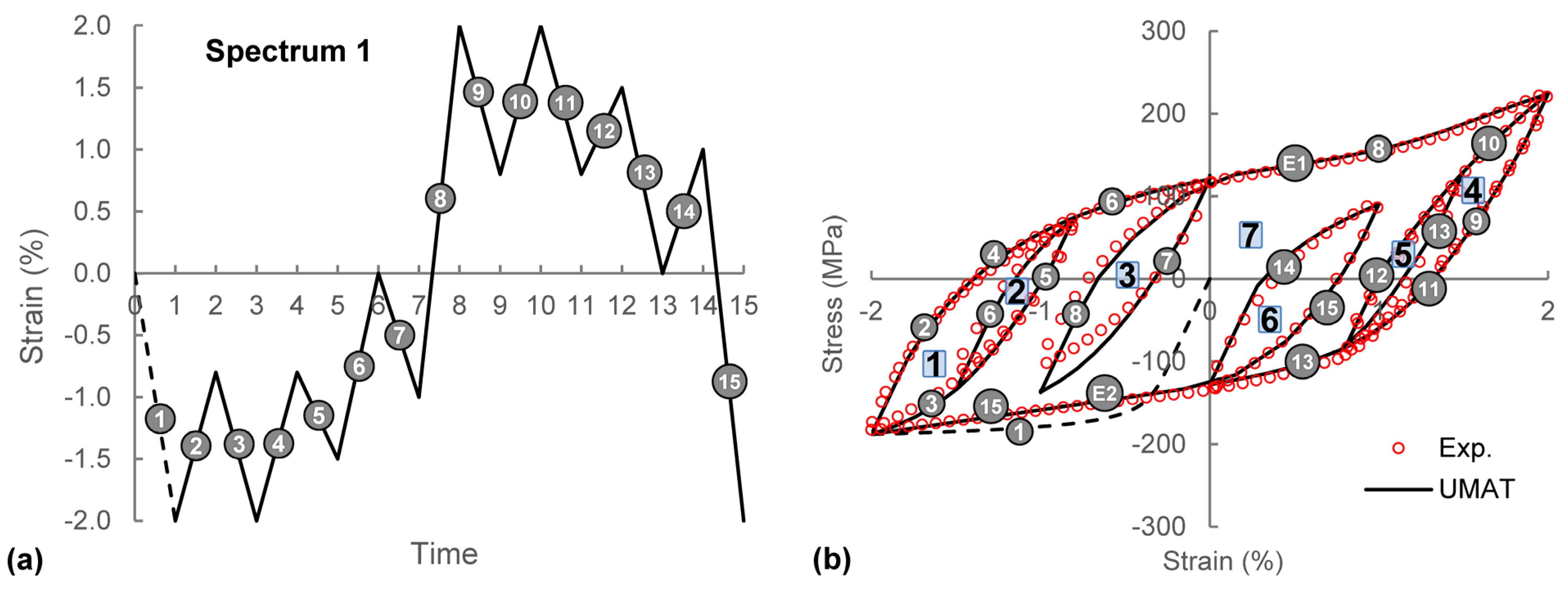
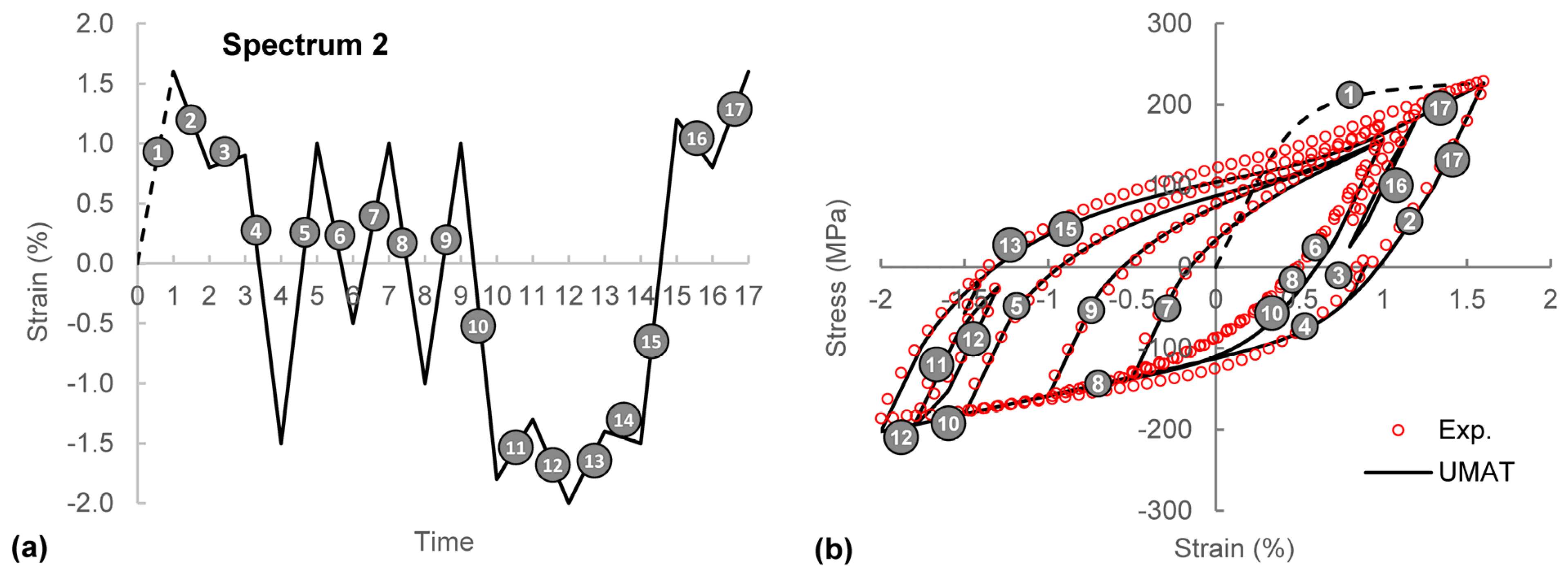
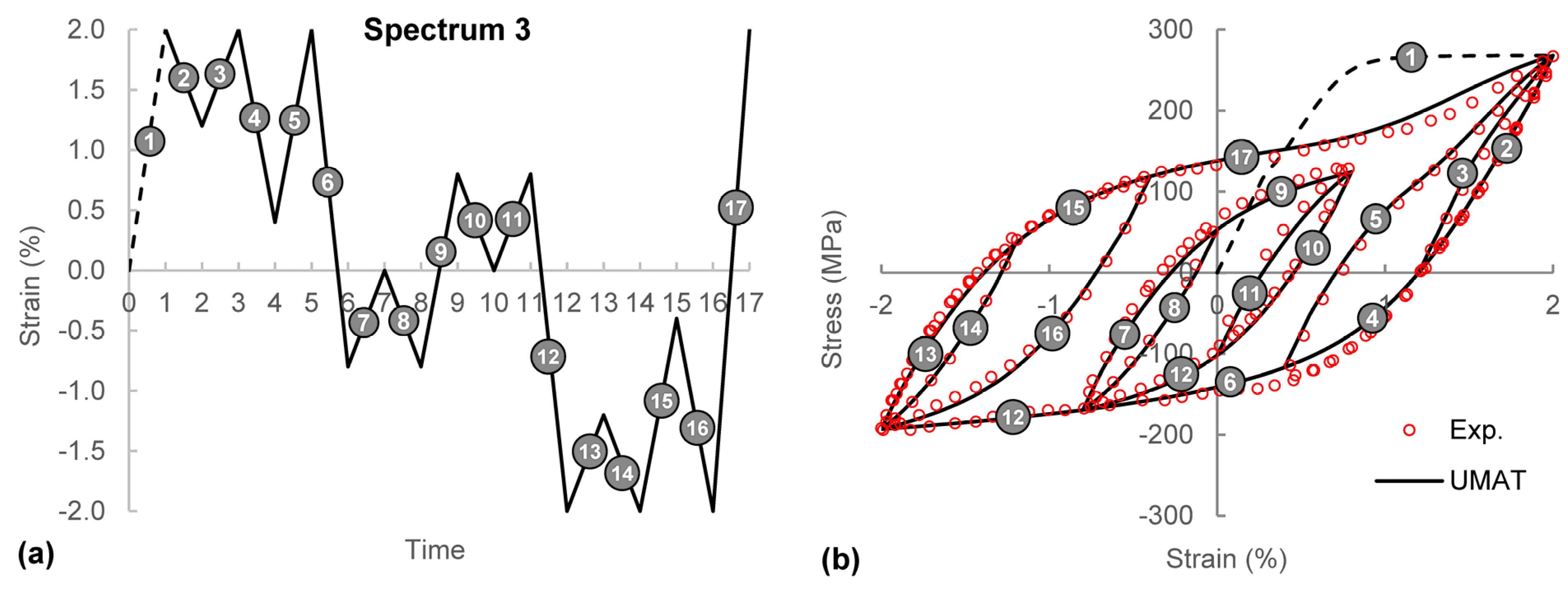
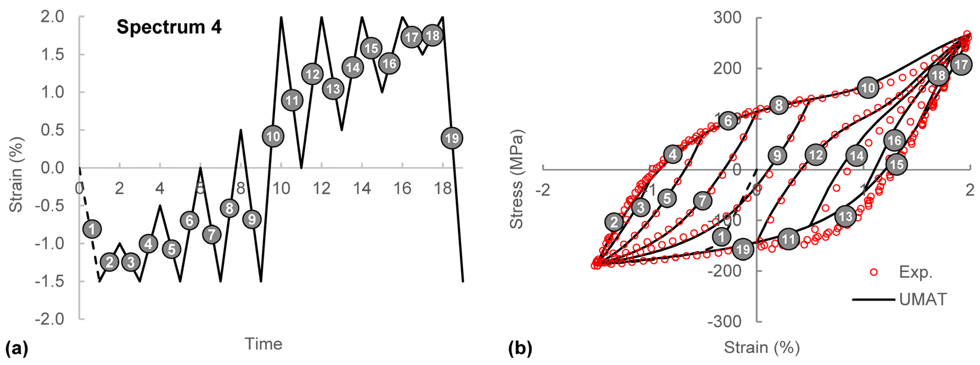
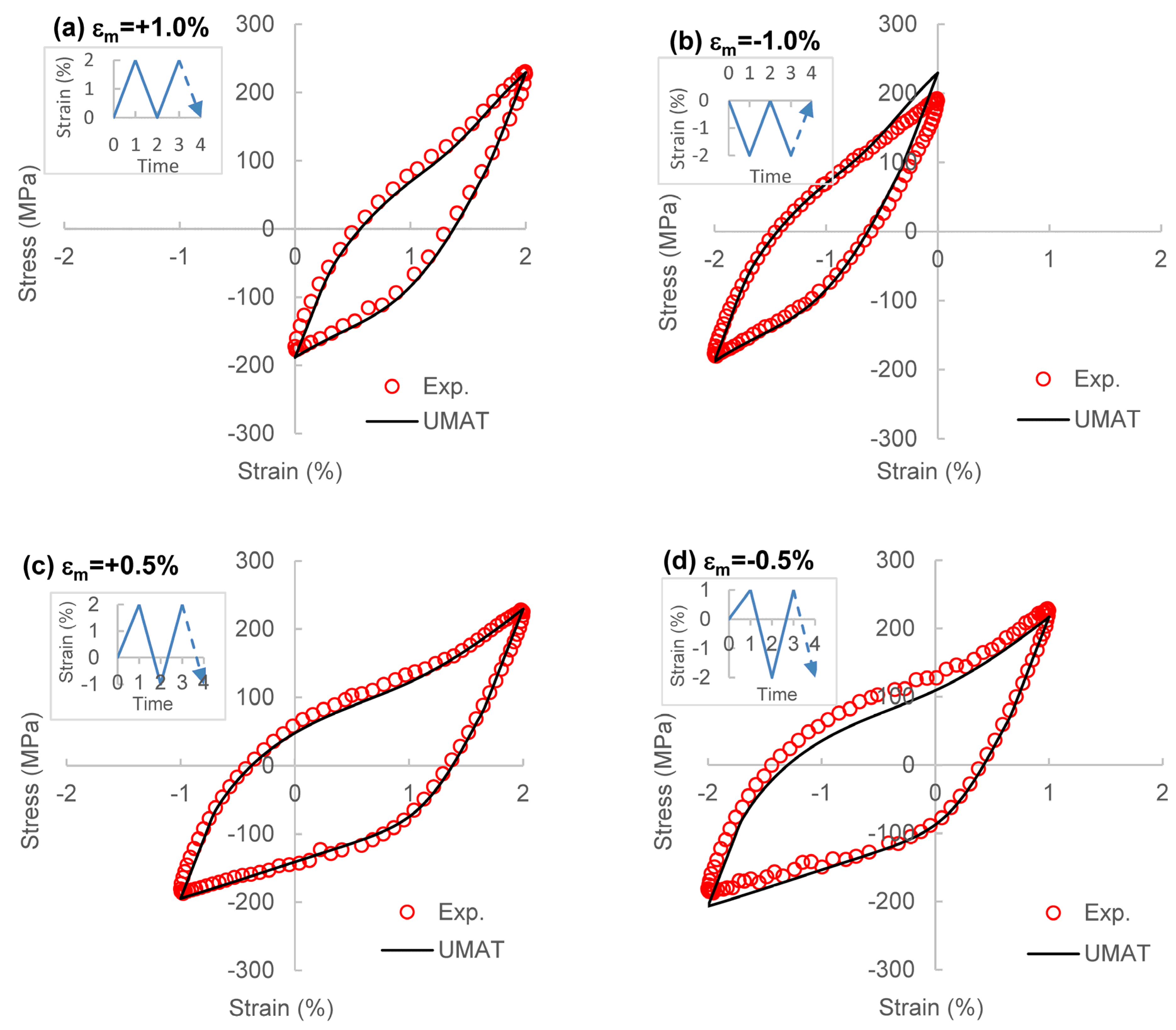
4.2. Variable Amplitude Loading

To verify the constitutive model under VAL, four different uniaxial cyclic tests were conducted on ZEK100 (spectrums 1 and 2) and AZ31B (spectrums 3 and 4). Figure 16, Figure 17, Figure 18 and Figure 19 display the loading spectrums and the comparison between the stabilized cyclic responses obtained from the experiment and the model. In these figures, the circled numbers denote the reversal number, and the squared numbers represent the cycle number.

Figure 16a shows a VAL strain spectrum, spectrum 1, which was applied to ZEK100. A loading block in this spectrum includes 15 reversals, which start with compressive loading. The spectrum contains an envelope cycle with a symmetric peak and valley strain of ±2%, cycle #7, and 6 inner cycles with asymmetric strain peaks and different tensile and compressive pre-strains, cycle #1–6. The input loading spectrum is modified by adding an envelope cycle after the first reversal, i.e., reversals E1 and E2, as explained in Section 2.1.4. The rearrangement of the loading spectrum is solely for the sake of finding the stabilized residual twin and the accumulated slip deformations, and not for cycle counting and damage calculations.

Figure 16. UMAT verification under VAL for ZEK100 (a) strain spectrum 1; (b) stabilized stress–strain response.

Figure 16. UMAT verification under VAL for ZEK100 (a) strain spectrum 1; (b) stabilized stress–strain response.

Figure 16b compares the stabilized hysteresis response obtained from the experiment with the simulation results. This graph demonstrates that the model was generally capable of explaining the cyclic behavior of the material under the VAL block. For the envelope cycle, cycle #7, the peak stresses as well as the hardening curves were captured successfully. This finding implies that the inner cycles within a VAL block do not affect the bounding cycle, as it follows the same hardening curves as for constant amplitude loading under the same strain level. This behavior is explained by the model due to the assumption that the hardening curves are governed by the residual deformations, which remain unchanged after the inner cycles are closed. The stabilized behavior for the inner cycles, in general, was well described in upward and downward reversals. Peak stresses and hardening behavior in upward reversals were explained successfully; including the upward reversals that close the previous (downward) reversals, e.g., reversals 4, 6, 10, and the upward reversals that remain open, i.e., virtually close the earlier downward reversals, e.g., reversal 14. The good agreement between the experiment and the UMAT for upward reversals demonstrates that the stabilized hardening behavior is effectively explained by the residual twin deformation and the constraint that the current reversal has to close the most recent open reversal. The stabilized response for downward reversals was captured well for reversals that close the last (upward) reversal, e.g., reversals 3, 11, 13, and 15. However, for the downward reversals that remain open, e.g., reversal 7, the simulation results slightly deviate from the experiment. The reason is that the hardening curve for downward reversals is determined from the accumulated slip deformation, which remains constant after the envelope cycle is closed. Thus, the only factor that allows for various downward flow curves during VAL is the constraint that the envelope cycle as well as the inner cycles form close loops. Therefore, as one would expect, the hardening curve for open downward reversals may not be captured as precisely as closed downward reversals.

Figure 17, Figure 18 and Figure 19 display the comparison between the UMAT predictions and the experiment for three other VAL spectrums, to further verify the proposed cyclic plasticity model. Overall, the UMAT was successful in predicting the stabilized cyclic behavior under various load cases for both ZEK100 and AZ31B. Spectra 2 to 4 are load cases where the envelope cycle has negative, zero, and positive mean strains, respectively. For spectrum 3, with no mean strain, the agreement between the simulation and experimental results was slightly superior to those for spectra 2 and 4, with non-zero mean strains. For loading spectra without mean strains, the hardening curves are directly obtained from the input fully-reversed hysteresis loops. However, the determination of the stabilized response for an envelope cycle with a non-zero mean strain relies on the assumption/rule that the hardening curve is governed by the strain range. Spectrum 2 includes elastic inner cycles, i.e., reversals 3–4 and 13–14, which are branching from downward or upward reversals, respectively. Also, this spectrum consists of inner cycles with minimal plastic strains, i.e., reversals 11–12 and 16–17. These cycles were captured by the model with reasonable accuracy. For inner cycles with significant plastic deformation, the minor deviation of the model predictions from the experiment (harder than the experiment in downward reversals and softer in upward reversals) was expected for spectra with negative mean strains, according to Figure 15d.

Figure 17. UMAT verification under VAL for ZEK100 (a) strain spectrum 2; (b) stabilized stress–strain response.

Figure 17. UMAT verification under VAL for ZEK100 (a) strain spectrum 2; (b) stabilized stress–strain response.

Spectrum 3, depicted in Figure 18a, was applied to AZ31B, and the material response for the stabilized loading block is shown in Figure 18b. This spectrum includes an envelope cycle without mean strain and seven inner cycles with various strain ranges. The inner cycles include the ones that form with two consecutive reversals, and a cycle that is formed by two reversals with an interval, i.e., reversals 9 and 12. The peak stresses and the hardening curves were closely predicted for the envelope cycle and all the inner cycles. For reversal 12, which closes the most recent open reversal (reversal 9) and continues, the stress–strain response after the closure of the cycle was well explained.

Figure 18. UMAT verification under VAL for AZ31B (a) strain spectrum 3; (b) stabilized stress–strain response.

Figure 18. UMAT verification under VAL for AZ31B (a) strain spectrum 3; (b) stabilized stress–strain response.

Figure 19 displays another VAL block and the stabilized response for AZ31B. This loading was intended to further verify the capability of the model to predict the material response under a VAL load case with a non-zero mean strain for the envelope cycle and various strain amplitudes for inner cycles, which are branched from both the upward and downward reversals. The inner cycles in this spectrum include four pairs of cycles, which are equal in strain range. For instance, the strain range for cycles #1 and 8 is 0.5%, and for cycles #2 and 7 it is 1.0%, etc. For each pair of cycles having the same strain range, the hardening curve for upward and downward reversals is significantly different. Figure 19b demonstrates that the proposed model is capable of successfully capturing this behavior, and further confirms that the residual plastic deformations can effectively describe the stabilized cyclic behavior.

Figure 19. UMAT verification under VAL for AZ31B (a) strain spectrum 4; (b) stabilized stress–strain response.

Figure 19. UMAT verification under VAL for AZ31B (a) strain spectrum 4; (b) stabilized stress–strain response.

In summary, the verification tests above suggest that the proposed cyclic plasticity model along with the rules introduced to generate the stabilized cyclic response, effectively explains the response of wrought Mg alloys with asymmetric hardening behavior under uniaxial VAL.

5. Conclusions

The present research proposed a cyclic plasticity model to describe the stabilized cyclic response of wrought Mg alloys. The model was implemented into a UMAT subroutine, calibrated, and verified for ZEK100 and AZ31B-H24 magnesium sheets. The following conclusions can be drawn from this research:

• A cyclic plasticity constitutive model was developed by adopting the symmetric von Mises yield criterion. The asymmetric initial yield strengths were described by virtually sub-sizing the yield surface. A novel combined isotropic–kinematic hardening rule was proposed for uniaxial loading.
• A procedure was introduced to generate the effective cyclic flow curves for an arbitrary cycle using a few fully-reversed hysteresis responses and the concepts of residual twin and accumulated slip deformations.
• According to the nature of the stabilized cyclic response of materials, the rules required to explain the stabilized hardening behavior were identified and incorporated into the plasticity model.
• The proposed constitutive model was calibrated for ZEK100 and AZ31B sheets. It was demonstrated that the UMAT was successful in reproducing the cyclic stress–strain behavior of the materials. The asymmetric initial yield strength, asymmetric hardening behavior, the Bauschinger effect, and reverse loading were well explained by the model.
• Within the scope of the verifications performed in this research, it was shown that the constitutive model was able to successfully describe the asymmetric cyclic hardening behavior of AZ31B and ZEK100 under constant amplitude loading with positive or negative mean strains. Moreover, the capability of the proposed model to predict the stabilized cyclic behavior of the materials under variable amplitude loading was verified.

References

1. Rodney, D.; Ventelon, L.; Clouet, E.; Pizzagalli, L.; Willaime, F. Ab Initio Modeling of Dislocation Core Properties in Metals and Semiconductors. Acta Mater. 2017, 124, 633–659. [Google Scholar] [CrossRef]
2. Staroselsky, A.; Anand, L. A Constitutive Model for Hcp Materials Deforming by Slip and Twinning: Application to Magnesium Alloy AZ31B. Int. J. Plast. 2003, 19, 1843–1864. [Google Scholar] [CrossRef]
3. Abdolvand, H.; Majkut, M.; Oddershede, J.; Schmidt, S.; Lienert, U.; Diak, B.J.; Withers, P.J.; Daymond, M.R. On the Deformation Twinning of Mg AZ31B: A Three-Dimensional Synchrotron X-Ray Diffraction Experiment and Crystal Plasticity Finite Element Model. Int. J. Plast. 2015, 70, 77–97. [Google Scholar] [CrossRef]
4. Castelluccio, G.M.; McDowell, D.L. Mesoscale Cyclic Crystal Plasticity with Dislocation Substructures. Int. J. Plast. 2017, 98, 1–26. [Google Scholar] [CrossRef]
5. Bong, H.J.; Lee, J.; Lee, M.-G. Modeling Crystal Plasticity with an Enhanced Twinning–Detwinning Model to Simulate Cyclic Behavior of AZ31B Magnesium Alloy at Various Temperatures. Int. J. Plast. 2022, 150, 103190. [Google Scholar] [CrossRef]
6. Jahed, H.; Roostaei, A. Cyclic Plasticity of Metals: Modeling Fundamentals and Applications; Jahed, H., Roostaei, A., Eds.; Elsevier: Amsterdam, The Netherlands, 2022; ISBN 9780128192931. [Google Scholar]
7. Prager, W. A New Method of Analyzing Stresses and Strains in Work-Hardening Plastic Solids. J. Appl. Mech. 1956, 23, 493–496. [Google Scholar] [CrossRef]
8. Mroz, Z. On the Description of Anisotropic Workhardening. J. Mech. Phys. Solids 1967, 15, 163–175. [Google Scholar] [CrossRef]
9. Lee, J.Y.; Lee, M.G.; Barlat, F.; Bae, G. Piecewise Linear Approximation of Nonlinear Unloading-Reloading Behaviors Using a Multi-Surface Approach. Int. J. Plast. 2017, 93, 112–136. [Google Scholar] [CrossRef]
10. Khutia, N.; Dey, P.P.; Sivaprasad, S.; Tarafder, S. Development of New Cyclic Plasticity Model for 304LN Stainless Steel through Simulation and Experimental Investigation. Mech. Mater. 2014, 78, 85–101. [Google Scholar] [CrossRef]
11. Krieg, R.D. A Practical Two Surface Plasticity Theory. J. Appl. Mech. 1975, 42, 641. [Google Scholar] [CrossRef]
12. Dafalias, Y.F.; Popov, E.P. Plastic Internal Variables Formalism of Cyclic Plasticity. J. Appl. Mech. 1976, 43, 645. [Google Scholar] [CrossRef]
13. Lee, M.G.G.; Kim, D.; Kim, C.; Wenner, M.L.L.; Wagoner, R.H.H.; Chung, K. A Practical Two-Surface Plasticity Model and Its Application to Spring-Back Prediction. Int. J. Plast. 2007, 23, 1189–1212. [Google Scholar] [CrossRef]
14. Yoshida, F.; Uemori, T. A Model of Large-Strain Cyclic Plasticity Describing the Bauschinger Effect and Workhardening Stagnation. Int. J. Plast. 2002, 18, 661–686. [Google Scholar] [CrossRef]
15. Kondori, B.; Madi, Y.; Besson, J.; Benzerga, A.A. Evolution of the 3D Plastic Anisotropy of HCP Metals: Experiments and Modeling. Int. J. Plast. 2018, 117, 71–92. [Google Scholar] [CrossRef]
16. Dafalias, Y.F. On Cyclic and Anisotropic Plasticity: (I) A General Model Including Material Behavior Under Stress Reversals. (II) Anisotropic Hardening for Initially Orthotropic Materials; University of California: Berkeley, CA, USA, 1975. [Google Scholar]
17. Chaboche, J.L. Time-Independent Constitutive Theories for Cyclic Plasticity. Int. J. Plast. 1986, 2, 149–188. [Google Scholar] [CrossRef]
18. Dafalias, Y.F. Bounding Surface Plasticity. I: Mathematical Foundation and Hypoplasticity. J. Eng. Mech. 1986, 112, 966–987. [Google Scholar] [CrossRef]
19. Frederick, C.O.; Armstrong, P.J. A Mathematical Representation of the Multiaxial Bauschinger Effect; Berkeley Nuclear Laboratories: Berkeley, CA, USA, 1966; Volume 731. [Google Scholar]
20. Ohno, N.; Wang, J.-D. Nonlinear Kinematic Hardening Rule with Critical State for Activation of Dynamic Recovery. In Anisotropy and Localization of Plastic Deformation; Springer: Dordrecht, The Netherlands, 1991; pp. 455–458. [Google Scholar]
21. Jiang, Y.; Sehitoglu, H. Modeling of Cyclic Ratchetting Plasticity, Part I: Development of Constitutive Relations. J. Appl. Mech. 1996, 63, 720–725. [Google Scholar] [CrossRef]
22. Abdel-Karim, M.; Ohno, N. Kinematic Hardening Model Suitable for Ratchetting with Steady-State. Int. J. Plast. 2000, 16, 225–240. [Google Scholar] [CrossRef]
23. Kang, G.; Kan, Q. Cyclic Plasticity of Engineering Materials: Experiments and Models; John Wiley & Sons: Hoboken, NJ, USA, 2017. [Google Scholar]
24. Hazeli, K.; Askari, H.; Cuadra, J.; Streller, F.; Carpick, R.W.; Zbib, H.M.; Kontsos, A. Microstructure-Sensitive Investigation of Magnesium Alloy Fatigue. Int. J. Plast. 2015, 68, 55–76. [Google Scholar] [CrossRef]
25. Ghorbanpour, S.; McWilliams, B.A.; Knezevic, M. Low-Cycle Fatigue Behavior of Rolled WE43-T5 Magnesium Alloy. Fatigue. Fract. Eng. Mater. Struct. 2019, 42, 1357–1372. [Google Scholar] [CrossRef]
26. Roostaei, A.A.; Jahed, H. Role of Loading Direction on Cyclic Behaviour Characteristics of AM30 Extrusion and Its Fatigue Damage Modelling. Mater. Sci. Eng. A 2016, 670, 26–40. [Google Scholar] [CrossRef]
27. Barlat, F.; Gracio, J.J.; Lee, M.-G.G.; Rauch, E.F.; Vincze, G. An Alternative to Kinematic Hardening in Classical Plasticity. Int. J. Plast. 2011, 27, 1309–1327. [Google Scholar] [CrossRef]
28. Kim, J.H.; Kim, D.; Lee, Y.-S.; Lee, M.-G.; Chung, K.; Kim, H.-Y.; Wagoner, R.H. A Temperature-Dependent Elasto-Plastic Constitutive Model for Magnesium Alloy AZ31 Sheets. Int. J. Plast. 2013, 50, 66–93. [Google Scholar] [CrossRef]
29. Hill, R. A Theory of the Yielding and Plastic Flow of Anisotropic Metals. Proc. R Soc. Lond. A Math. Phys. Sci. 1948, 193, 281–297. [Google Scholar]
30. Cazacu, O.; Plunkett, B.; Barlat, F. Orthotropic Yield Criterion for Hexagonal Closed Packed Metals. Int. J. Plast. 2006, 22, 1171–1194. [Google Scholar] [CrossRef]
31. Nguyen, N.-T.; Lee, M.-G.; Kim, J.H.; Kim, H.Y. A Practical Constitutive Model for AZ31B Mg Alloy Sheets with Unusual Stress–Strain Response. Finite Elem. Anal. Des. 2013, 76, 39–49. [Google Scholar] [CrossRef]
32. Muhammad, W.; Mohammadi, M.; Kang, J.; Mishra, R.K.; Inal, K. An Elasto-Plastic Constitutive Model for Evolving Asymmetric/Anisotropic Hardening Behavior of AZ31B and ZEK100 Magnesium Alloy Sheets Considering Monotonic and Reverse Loading Paths. Int. J. Plast. 2015, 70, 30–59. [Google Scholar] [CrossRef]
33. Li, M. Constitutive Modeling of Slip, Twinning, and Untwinning in AZ31B Magnesium; The Ohio State University: Columbus, OH, USA, 2006. [Google Scholar]
34. Li, M.; Lou, X.Y.; Kim, J.H.; Wagoner, R.H. An Efficient Constitutive Model for Room-Temperature, Low-Rate Plasticity of Annealed Mg AZ31B Sheet. Int. J. Plast. 2010, 26, 820–858. [Google Scholar] [CrossRef]
35. Lee, M.G.; Wagoner, R.H.; Lee, J.K.; Chung, K.; Kim, H.Y. Constitutive Modeling for Anisotropic/Asymmetric Hardening Behavior of Magnesium Alloy Sheets. Int. J. Plast. 2008, 24, 545–582. [Google Scholar] [CrossRef]
36. Lee, M.G.; Kim, S.J.; Wagoner, R.H.; Chung, K.; Kim, H.Y. Constitutive Modeling for Anisotropic/Asymmetric Hardening Behavior of Magnesium Alloy Sheets: Application to Sheet Springback. Int. J. Plast. 2009, 25, 70–104. [Google Scholar] [CrossRef]
37. Drucker, D.C.; Prager, W. Soil Mechanics and Plastic Analysis or Limit Design. Q Appl. Math. 1952, 10, 157–165. [Google Scholar] [CrossRef]
38. He, Z.; Chen, W.; Wang, F.; Feng, M. A Kinematic Hardening Constitutive Model for the Uniaxial Cyclic Stress–Strain Response of Magnesium Sheet Alloys at Room Temperature. Mater. Res. Express. 2017, 4, 116513. [Google Scholar] [CrossRef]
39. Noban, M.; Albinmousa, J.; Jahed, H.; Lambert, S. A Continuum-Based Cyclic Plasticity Model for AZ31B Magnesium Alloy under Proportional Loading. Procedia. Eng. 2011, 10, 1366–1371. [Google Scholar] [CrossRef]
40. Roostaei, A.A.; Jahed, H. A Cyclic Small-Strain Plasticity Model for Wrought Mg Alloys under Multiaxial Loading: Numerical Implementation and Validation. Int. J. Mech. Sci. 2018, 145, 318–329. [Google Scholar] [CrossRef]
41. Anes, V.; Moreira, R.; Reis, L.; Freitas, M. Simulation of the Cyclic Stress–Strain Behavior of the Magnesium Alloy AZ31B-F under Multiaxial Loading. Crystals 2023, 13, 969. [Google Scholar] [CrossRef]
42. Kang, G.; Li, H. Review on Cyclic Plasticity of Magnesium Alloys: Experiments and Constitutive Models. Int. J. Miner. Metall. Mater. 2021, 28, 567–589. [Google Scholar] [CrossRef]
43. Casey, J.; JahedMotlagh, H. The Strength-Differential Effect in Plasticity. Int. J. Solids Struct. 1984, 20, 377–393. [Google Scholar] [CrossRef]
44. Stephens, R.I.; Fatemi, A.; Stephens, R.R.; Fuchs, H.O. Metal Fatigue in Engineering; John Wiley & Sons: New York, NY, USA, 2001; p. 496. [Google Scholar]
45. Wu, L.; Jain, A.; Brown, D.W.W.; Stoica, G.M.M.; Agnew, S.R.R.; Clausen, B.; Fielden, D.E.E.; Liaw, P.K.K. Twinning–Detwinning Behavior during the Strain-Controlled Low-Cycle Fatigue Testing of a Wrought Magnesium Alloy, ZK60A. Acta Mater. 2008, 56, 688–695. [Google Scholar] [CrossRef]
46. Shi, R.; Zheng, J.; Li, T.; Shou, H.; Yin, D.; Rao, J. Quantitative Analysis of the Deformation Modes and Cracking Modes during Low-Cycle Fatigue of a Rolled AZ31B Magnesium Alloy: The Influence of Texture. Mater. Sci. Eng. A 2022, 844, 143103. [Google Scholar] [CrossRef]
47. Lei, Y.; Li, H.; Liu, Y.; Wang, Z.; Kang, G. Experimental Study on Uniaxial Ratchetting-Fatigue Interaction of Extruded AZ31 Magnesium Alloy with Different Plastic Deformation Mechanisms. J. Magnes. Alloys 2023, 11, 379–391. [Google Scholar] [CrossRef]
48. Ziegler, H. A Modification of Prager’s Hardening Rule. Quarternery Appl. Math. 1959, 17, 55–65. [Google Scholar] [CrossRef]
49. Lv, F.; Yang, F.; Duan, Q.Q.Q.; Yang, Y.S.S.; Wu, S.D.D.; Li, S.X.X.; Zhang, Z.F.F. Fatigue Properties of Rolled Magnesium Alloy (AZ31) Sheet: Influence of Specimen Orientation. Int. J. Fatigue. 2011, 33, 672–682. [Google Scholar] [CrossRef]
50. Lv, F.; Yang, F.; Duan, Q.Q.; Luo, T.J.; Yang, Y.S.; Li, S.X.; Zhang, Z.F. Tensile and Low-Cycle Fatigue Properties of Mg–2.8% Al–1.1% Zn–0.4% Mn Alloy along the Transverse and Rolling Directions. Scr. Mater. 2009, 61, 887–890. [Google Scholar] [CrossRef]
51. Park, S.H.; Hong, S.G.; Bang, W.; Lee, C.S. Effect of Anisotropy on the Low-Cycle Fatigue Behavior of Rolled AZ31 Magnesium Alloy. Mater. Sci. Eng. A 2010, 527, 417–423. [Google Scholar] [CrossRef]
52. Lin, Y.C.; Liu, Z.H.; Chen, X.M.; Long, Z.L. Cyclic Plasticity Constitutive Model for Uniaxial Ratcheting Behavior of AZ31B Magnesium Alloy. J. Mater. Eng. Perform. 2015, 24, 1820–1833. [Google Scholar] [CrossRef]
53. Cazacu, O.; Barlat, F. A Criterion for Description of Anisotropy and Yield Differential Effects in Pressure-Insensitive Metals. Int. J. Plast. 2004, 20, 2027–2045. [Google Scholar] [CrossRef]
54. Chen, L.; Zhang, J.; Zhang, H. Anisotropic Yield Criterion for Metals Exhibiting Tension–Compression Asymmetry. Adv. Appl. Math. Mech. 2021, 13, 701–723. [Google Scholar] [CrossRef]
55. Yang, Q.; Jiang, B.; Song, B.; Yu, Z.; He, D.; Chai, Y.; Zhang, J.; Pan, F. The Effects of Orientation Control via Tension-Compression on Microstructural Evolution and Mechanical Behavior of AZ31 Mg Alloy Sheet. J. Magnes. Alloys 2022, 10, 411–422. [Google Scholar] [CrossRef]
56. Mekonen, M.N.; Steglich, D.; Bohlen, J.; Letzig, D.; Mosler, J. Mechanical Characterization and Constitutive Modeling of Mg Alloy Sheets. Mater. Sci. Eng. A 2012, 540, 174–186. [Google Scholar] [CrossRef]
57. Kim, J.; Ryou, H.; Kim, D.D.D.; Lee, W.; Hong, S.-H.H.; Chung, K.; Kim, D.D.D.; Lee, W.; Hong, S.-H.H.; Chung, K. Constitutive Law for AZ31B Mg Alloy Sheets and Finite Element Simulation for Three-Point Bending. Int. J. Mech. Sci. 2008, 50, 1510–1518. [Google Scholar] [CrossRef]
58. Nixon, M.E.; Cazacu, O.; Lebensohn, R.A. Anisotropic Response of High-Purity α-Titanium: Experimental Characterization and Constitutive Modeling. Int. J. Plast. 2010, 26, 516–532. [Google Scholar] [CrossRef]
59. Lee, J.-W.; Lee, M.-G.; Barlat, F. Finite Element Modeling Using Homogeneous Anisotropic Hardening and Application to Spring-Back Prediction. Int. J. Plast. 2012, 29, 13–41. [Google Scholar] [CrossRef]
60. Hasegawa, S.; Tsuchida, Y.; Yano, H.; Matsui, M. Evaluation of Low Cycle Fatigue Life in AZ31 Magnesium Alloy. Int. J. Fatigue. 2007, 29, 1839–1845. [Google Scholar] [CrossRef]
61. Li, Q.; Yu, Q.; Zhang, J.; Jiang, Y. Effect of Strain Amplitude on Tension-Compression Fatigue Behavior of Extruded Mg6Al1ZnA Magnesium Alloy. Scr. Mater. 2010, 62, 778–781. [Google Scholar] [CrossRef]
62. Jordon, J.B.; Gibson, J.B.; Horstemeyer, M.F.; Kadiri, H.E.; Baird, J.C.; Luo, A.A. Effect of Twinning, Slip, and Inclusions on the Fatigue Anisotropy of Extrusion-Textured AZ61 Magnesium Alloy. Mater. Sci. Eng. A 2011, 528, 6860–6871. [Google Scholar] [CrossRef]
63. Behravesh, S.B. Fatigue Characterization and Cyclic Plasticity Modeling of Magnesium Spot-Welds; University of Waterloo: Waterloo, ON, Canada, 2013. [Google Scholar]
64. Jiang, Y.; Zhang, J. Benchmark Experiments and Characteristic Cyclic Plasticity Deformation. Int. J. Plast. 2008, 24, 1481–1515. [Google Scholar] [CrossRef]
65. Yu, Q.; Zhang, J.; Jiang, Y.; Li, Q. An Experimental Study on Cyclic Deformation and Fatigue of Extruded ZK60 Magnesium Alloy. Int. J. Fatigue. 2012, 36, 47–58. [Google Scholar] [CrossRef]
66. Yin, S.M.; Yang, H.J.; Li, S.X.; Wu, S.D.; Yang, F. Cyclic Deformation Behavior of As-Extruded Mg-3%Al-1%Zn. Scr. Mater. 2008, 58, 751–754. [Google Scholar] [CrossRef]
67. Partridge, P.G. Cyclic Twinning in Fatigued Close-Packed Hexagonal Metals. Philos. Mag. 1965, 12, 1043–1054. [Google Scholar] [CrossRef]
68. Lou, X.Y.; Li, M.; Boger, R.K.; Agnew, S.R.; Wagoner, R.H. Hardening Evolution of AZ31B Mg Sheet. Int. J. Plast. 2007, 23, 44–86. [Google Scholar] [CrossRef]
69. Abaqus Analysis User’s Manual, Version 6.14-1; Dassault Systemes Simulia Inc.: Providence, RI, USA, 2014.
70. Ling, Y.; Roostaei, A.A.; Glinka, G.; Jahed, H. Fatigue of ZEK100-F Magnesium Alloy: Characterisation and Modelling. Int. J. Fatigue. 2019, 125, 179–186. [Google Scholar] [CrossRef]
71. Behravesh, S.B.; Jahed, H.; Lambert, S. Fatigue Characterization and Modeling of AZ31B Magnesium Alloy Spot-Welds. Int. J. Fatigue. 2014, 64, 1–13. [Google Scholar] [CrossRef]
Figure 1. Schematic of cyclic tension and cyclic compression curves and the corresponding yield surface.
Metals 14 00221 g001
Figure 2. Interpolation between upward and downward reversals of stabilized hysteresis loops obtained from fully-reversed strain-controlled tests; (a,c) experimentally obtained uniaxial hysteresis loops under two different strain amplitudes; (b,d) downward and upward reversals hardening curves translated to the origin, and interpolated curves.
Metals 14 00221 g002
Figure 3. Stabilized hysteresis response of AZ31B under uniaxial cyclic loading with strain amplitude of ε a = 1.5% [63] highlighting the yield stresses in upward and downward reversals.
Metals 14 00221 g003
Figure 4. Schematic illustration of the hardening rule in the reference frame (a); effective flow curve for an upward reversal (b); evolution of the reference yield surface under uniaxial tension; (c) effective flow curve for a downward reversal; (d) evolution of the reference yield surface under uniaxial compression.
Metals 14 00221 g004
Figure 5. Reverse loading criterion.
Metals 14 00221 g005
Figure 6. Sudden change in elastic region size after reverse loading.
Metals 14 00221 g006
Figure 7. Yield surface shrinkage and back stress change upon reverse loading under uniaxial load.
Metals 14 00221 g007
Figure 8. Modeling the stabilized hysteresis response under VAL (a) an arbitrary input VAL spectrum; (b) modified spectrum with the envelope cycle added; (c) stabilized hysteresis response under VAL.
Metals 14 00221 g008
Figure 9. (a) Specimen geometry for ZEK100; (b) anti-buckling fixture for ZEK100; (c) specimen geometry for AZ31B (all dimensions are ‘mm’, except the surface roughness which is micron).
Metals 14 00221 g009
Figure 10. Schematic illustration of the sigmoid function and its parameters.
Metals 14 00221 g010
Figure 11. (a) Stabilized hysteresis loops under different strain amplitudes; (b) uniaxial cyclic curves for ZEK100 (dashed lines represent the elastic region under cyclic loading).
Metals 14 00221 g011
Figure 12. Stabilized hysteresis response for ZEK100 under different strain amplitudes; comparison between the model predictions and the experiments.
Metals 14 00221 g012
Figure 13. (a) Stabilized hysteresis loops under different strain amplitudes; (b) uniaxial cyclic curves for AZ31B (dashed lines represent the elastic region under cyclic loading).
Metals 14 00221 g013
Figure 14. Stabilized hysteresis response for AZ31B under different strain amplitudes; comparison between model predictions and experiments.
Metals 14 00221 g014
Figure 15. Model verification for ZEK100 under constant amplitude loading with non-zero mean strain (a) TCT, ε m a x = +2%, ε m i n = 0; (b) CTC, ε m a x = 0, ε m i n = −2%; (c) TCT, ε m a x = +2%, ε m i n = −1%; (d) TCT, ε m a x = +1%, ε m i n = −2%.
Metals 14 00221 g015