Machine Learning-Assisted Prediction of Corrosion Behavior of 7XXX Aluminum Alloys

Abstract

High-strength and lightweight 7XXX Al alloys are widely applied in aerospace industries. Stress corrosion cracking (SCC) in these alloys has been extensively discussed, and electrochemical corrosion should be brought to the forefront when these materials are used in marine atmospheric environments. This work obtained the corrosion potentials (Ecorr) and corrosion rates of 40 as-cast 7XXX Al alloys by potentiodynamic polarization tests and immersion tests, respectively; then, chemical compositions and physical features were used to build a machine learning model to predict these parameters. RFR was used for the prediction model of Ecorr with the features Cu, Ti, Al, and Zn, and GPR for that of the corrosion rate with the features of specific heat, latent heat of fusion, and proportion of p electrons. The physical meaning and reasonability were discussed based on the analysis of corrosion morphology and precipitated composition. This work provides a reference for the design of corrosion-resistant 7XXX Al alloys and shows a method of conducting corrosion mechanism evaluation by using machine learning.

1. Introduction

By virtue of their high-strength and lightweight mechanic properties, 7XXX Al alloys are widely used in aerospace industries. When considering the application on shipboard aircraft, the widely researched SCC and electrochemical corrosion should be considered [1,2,3]. It is reported that the precipitated phase is a crucial factor influencing the mechanical properties and SCC of 7XXX Al alloys [2,4,5]. The heat treatment and element segregation are factors exerting a significant influence on the precipitated phases’ morphology and composition. Thus, to improve the corrosion resistance of 7XXX Al alloys, both these factors should be considered.

Recently, the materials science community has begun to utilize machine learning tools for tasks such as developing new materials [6] and evaluation mechanisms to predict the properties of materials [7,8,9]. Wen et al. [10] proposed a model to predict high-entropy alloys’ solid-solution strength based on feature extraction with a machine learning algorithm. Xue et al. [11] used machine learning for adaptive design to experimentally synthesize 36 alloy samples for predicting their components and discovered a novel, multi-component, Ni-Ti-based shape memory alloy with extremely low hysteresis from a compositional space containing approximately 800,000 different components. Stanev et al. [9] studied the importance of predictors in each superconducting system through machine learning and determined the physical mechanisms that drive superconductivity in different systems.

Machine learning models exhibit high prediction accuracy and robust fitting analysis ability in handling complex, nonlinear, and uncertain multi-dimensional features, leading to their proposed application in corrosion research. For example, Wei et al. [12] established a relationship model between the corrosion potential of Sanya seawater low-alloy steel and its influencing factors through an artificial neural network and visualized the influence of several alloying elements on the corrosion potential. Lv et al. [13] quantified the shape parameters of the steel section as input features and applied the PSO-SVM and GSSVM methods to accurately predict the corrosion rate of the section. Liu et al. [14] explored the influence of different seawater environments on the corrosion rate of 3c steel through a machine learning method and SHAP interpretation technology and found that the REDOX potential had the greatest impact on the corrosion rate and was positively correlated with it. Feng et al. [15] used a non-dominated sorting genetic machine learning algorithm to optimize the chemical composition of Al-Mg-Si alloy; they successfully developed high-performance alloys with low Mg, Si, and Cu contents, which improved the strength and corrosion resistance, and analyzed the effect their microstructure on performance improvement.

In recent years, there has been a notable shift in research focus towards using machine learning methods to explore the intrinsic connection between the microstructure and properties of materials. This new research direction aims to deepen our understanding of material properties and their influence. For instance, Ao et al. [16] proposed a deep learning strategy to predict the mechanical properties and corrosion behavior of large extruded aluminum profiles by using surface optical microstructure images and determined the precise correlations among metallographic images, hardness, and corrosion potential. Messina et al. [17] quantified the segregation ability of aluminum at magnesium grain boundaries by using atomic simulation and revealed the segregation influence of aluminum in the grain boundary structure and local atomic environment by training machine learning models. Ji et al. [18] proposed a strategy combining first-principles calculation with random forest (IACRF) to optimize the model to estimate the corrosion rate of aluminum alloys in diverse environments. Through the thermodynamic evaluation of intermetallic compounds and the use of first-principles calculations, the prediction accuracy of small-sample aluminum alloy corrosion data sets was improved. Takara et al. [19] studied the effect of intermetallic compound composition on the potential difference between aluminum alloy matrix and intermetallic compounds through machine learning, and the results showed that the potential difference had a linear relationship with the concentration of intermetallic compounds; in particular, the Cu element had a significant effect on the potential difference. It was also shown that by analyzing the relationship between smaller compounds and potential difference, it was possible to accurately evaluate the effect of compounds on aluminum alloy corrosion. These new research directions aim to reveal deeper mechanisms of the influence of material properties and provide a more comprehensive and in-depth understanding of advances in materials science.

While recent studies have successfully used machine learning techniques to predict the mechanical properties, corrosion behavior, and segregation effects of aluminum alloys, there are still challenges associated with experimental bias in data from the corrosion behavior literature. Thus, it is hard to extract useful information from the literature data.

In this study, we collected corrosion data from as-cast aluminum alloys prepared experimentally. Potentiodynamic polarization and immersion tests were performed to obtain corrosion potential (E_corr) and corrosion rates, respectively; then, the chemical compositions and physical features were used to establish a machine learning model to predict these parameters. Moreover, the features strongly related to E_corr and corrosion rates were extracted, and the physical meaning of the models was explained based on these features. Numerous studies have shown that the corrosion of aluminum alloys in chloride-containing solutions predominantly manifests as pitting corrosion [20,21,22]. The uniform corrosion rate used in this paper does not fully reflect the actual risk; however, as an attempt to predict aluminum alloy corrosion using machine learning, it holds academic significance. In future research, we will endeavor to quantify pitting behavior data and make predictions specifically targeting pitting corrosion.

2. Experimental Method and Dataset

2.1. Corrosion Dataset

For this work, 40 kinds of 7XXX series Al alloys were prepared by arc-melting the mixtures of high-purity (99.99%) aluminum and other doping elements in an argon atmosphere at 800 °C for 15 min and then cooled in air. Chemical composition analysis was performed for each specimen.

The potentiodynamic polarization tests were performed to obtain the corrosion potential (E_corr) in 3.5% NaCl solution at 25 °C by using Gamry interface 1000 after the open circuit potential (OCP) had reached the steady state. A three-electrode system was used in the electrochemical cell. A platinum plate and a saturated calomel electrode (SCE) were chosen as the counter and reference electrodes. A 7XXX series Al alloy specimen with an exposed surface area of 1 cm² was used as the working electrode. The samples’ potential was changed from an initial potential of −300 mV vs. E_OCP to 300 mV vs. E_OCP at a rate of 0.33 mV/s. Corrosion potential (Ecorr) and corrosion current density (icorr) were obtained from polarization curves by the Tafel extrapolation method. In this work, the exposed surface was polished by SiC paper, from #400 to #2000. Grinding resulted in a thickness reduction of about 0.5 mm, exposing the soaked surface of the electrode sample to various fiber textures. To ensure the repeatability of electrochemical measurements, 3 samples were tested in each group.

For the immersion tests, the material was cut into coupons with the dimensions 10 mm × 15 mm × 3 mm. The surface of each sample was polished with up to 2000 grit sandpaper and then degreased and cleaned with acetone and ethanol in an ultrasonic bath to remove dirt and any other foreign particles from the surface, which was then dried in flowing cool air. Grinding resulted in a thickness reduction of about 0.5 mm; all the samples (original samples) were weighed, and the surface area was measured.

The prepared specimens were immersed in 3.5% NaCl for 30 days at 25 °C. The weight gain or loss of the specimens was measured with a chemical balance with an accuracy of 0.0001 mg. We cleaned the samples according to ASTM standard G1-03. We weighed the control specimens before and after cleaning so that the extent of metal loss caused by cleaning could be used to correct the corrosion mass loss. After cleaning, we calculated the corrosion rates using the weight loss method with the formula below (Equation (1)), where K is a constant, D is the density of the Al alloys, A is the area of the specimens exposed in 3.5% NaCl solution, W is the weight loss or weight gain after the immersion test, and T is the duration of the immersion test [23].

$$Corrosion rate=\frac{K·W}{A·T·D}$$

(1)

After removing the corrosion products on the specimen’s surface, the corrosion morphology was analyzed by a scanning electron microscope (SEM) equipped with an energy-dispersive spectrometer (EDS) (SEM and EDS were provided by Zeiss, Oberkochen, Germany).

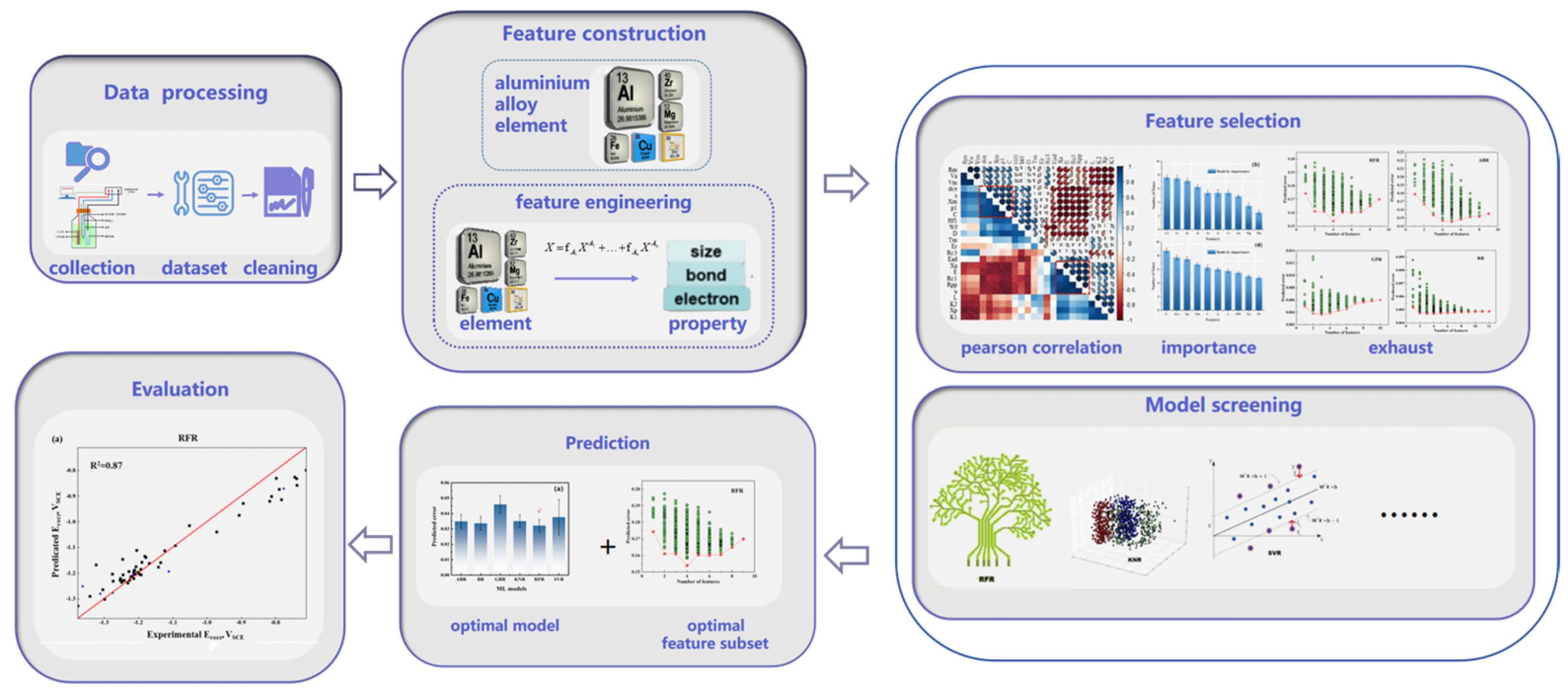
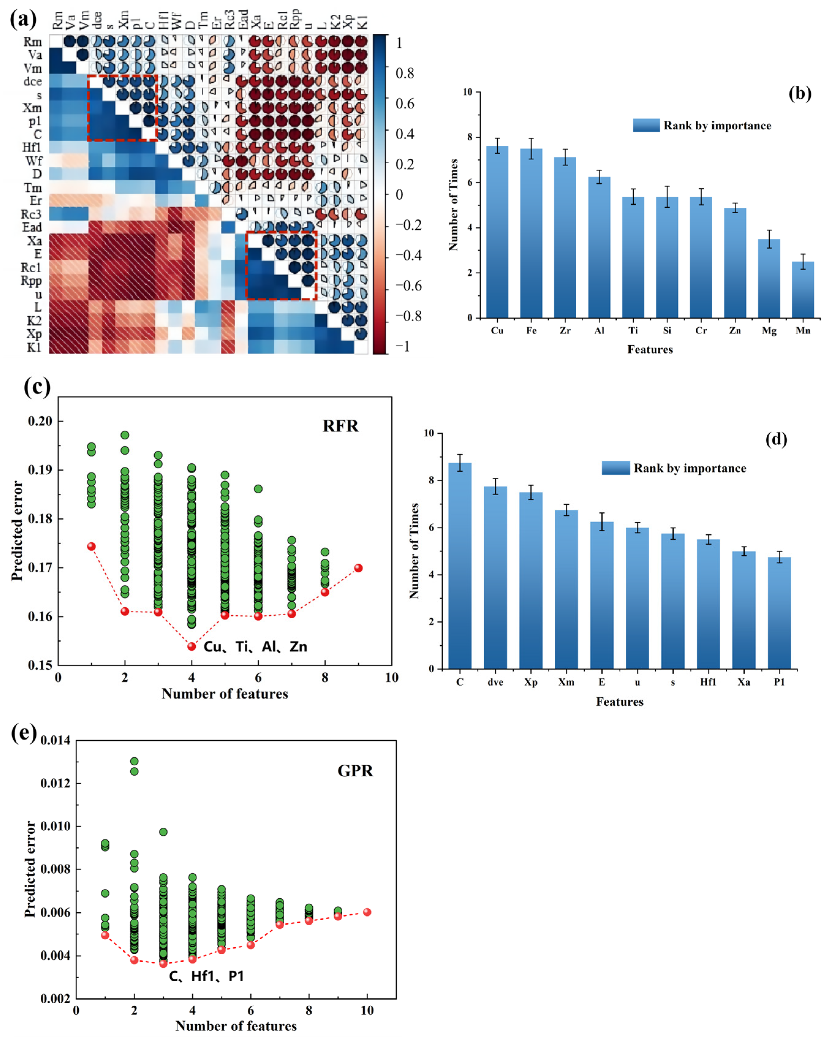
2.2. Feature Creation and Selection

In order to achieve high-precision machine learning prediction models, an in-depth understanding of material mechanisms, and efficient optimization of material design, we must scientifically and reasonably construct material characteristics that are closely related to the target quantity. When dealing with materials problems or target quantities in specific application scenarios, scholars [24,25,26] usually directly use material parameters as features to train machine learning models in combination with the problem background and existing knowledge. When establishing a machine learning model based on material characteristics as input, their high dimensionality and significant information redundancy often lead to overfitting issues. Prior materials knowledge is also utilized to perform mathematical operations on parameters such as the electronic, atomic, and crystallographic features of elements, as well as thermodynamic and kinetic parameters of materials. These parameters are transformed into factors to train machine learning models, enhancing the generalization ability of the latter [27,28].

In terms of feature creation, two groups of features were used to predict the corrosion rates and E_corr of the Al alloys. Group I included the chemical compositions, namely, the Al, Fe, Si, Mn, Cu, Ti, Zn, Mg, Cr, and Zr elements, which were used to predict E_corr. Group II included the physical features (X), created according to Equation (2). The atomic and physical property values for each element were obtained from the Webelements database.

$$X={\sum }_i^n{f}_i·x_i$$

(2)

where $f_i$ is the mass fraction of elements and $x_i$ represents the physical features of an atom, including distance of valence electrons (dve), distance of core electrons (dce), pseudo-potential radius (Rpp), covalent radius (Rc1), covalent radius 2 (Rc2), covalent radius 3 (Rc3), metal radius (Rm), melting temperature (Tm), second ionization energy (Eis), third ionization energy (Eit), electronic affinity (Ea), enthalpy vaporization (Env), latent heat of fusion (Hf1), latent heat of fusion 2 (Hf2), Miedema enthalpy of surface (Ens), Miedema enthalpy of vacancies (Env), work function (Wf), Brewer cohesive energy (Ec), total energy (Et), energy of the atomic orbitals (Eo3s), 2nd lowest energy of the atomic orbitals (Eol2), valence electrons of s orbital (s), proportion of p electrons (p1), effective nuclear charge (Nes), electronegativity (Xm, Xp, and Xa), compression modulus (L), bulk modulus (K1), bulk modulus 2 (K2), rigidity modulus (E), Young’s modulus (Ey1), Young’s modulus 2 (Ey2), thermal conductivity (Kt), resistivity 2 (Er), specific heat (C), electrical conductivity (Ec), thermal expansion (Te), atom volume (Va), atomic weight (u), molar volume (Vm), density (D), and cl⁻ adsorption energy (Ead). These features were used to predict the corrosion rate, as they represent coarse-grained simulations of the material’s electronic and bonding properties. This method has been used to predict the properties of shape memory alloys [11] and superconductors [9].

When constructing a machine learning model, the utilization of material features as inputs frequently encounters challenges associated with excessively high input variable dimensions and considerable information redundancy. These issues have the potential to cause overfitting in the model, thereby compromising its performance. To address these concerns, it is essential to engage in a process of filtering and screening the material characteristics, with the aim to enhance the stability and generalization capabilities of the model, ultimately leading to improved overall performance [29].

In this study, for Group II, including atomic and physical properties with higher dimensions (X), Pearson correlation coefficient analysis and forward–backward algorithm were used successively to screen the features. For Group I, given the limited number of features, the forward–backward algorithm was directly utilized for effective screening.

Following this, we utilized the exhaust algorithm to search and compute all feasible feature combinations that had passed the above screening phase. The objective of this step was to identify the subset of features exhibiting the low relative rest error rate in each machine learning model. We employed 10-fold cross-validation to assess individual machine learning models using different feature subsets.

2.3. Evaluation of Model Performance

In selecting the appropriate machine learning model, it is imperative to consider the model’s complexity, generalization capabilities, and the compatibility of data features. This balancing act is crucial to achieving both accuracy and robustness in material property predictions. Regression algorithms have gained widespread acceptance in predicting material properties [30,31]. To construct an effective model, it is necessary to customize the model to the specific materials problem and present multiple models for comparative evaluation and selection.

In this study, we systematically evaluated 16 different machine learning algorithms, including linear regression (LR), Bayesian regression (BR), elastic network regression (EN), lasso regression (LA), passive adversarial regression (PAR), ridge regression (RR), stochastic gradient descent regression (SGDR), Gaussian process regression (GPR), nearest-neighbor regression (KNR), nuclear ridge regression (KRR), multi-level perceptron (MLP), support vector regression (SVR), adaptive ensemble regression (ABR), decision tree regression (DTR), gradient lifting regression (GBR), and random forest regression (RFR).

All machine learning algorithms were executed in a Python environment using the scikit-learn library. To evaluate the predictive performance of the model based on specific features, we utilized the coefficient of determination (R²) and mean square error (MSE) as evaluation metrics, whose formulas are shown below in Equations (3) and (4). The coefficient of determination assesses how effectively the model elucidates the target variable, ranging from 0 to 1, with higher values indicating better model fit. The root mean square error gauges the variance between the model’s predicted values and the actual observed values; lower values signify higher prediction accuracy. The algorithm uses GridSearchCV to adjust the parameters step by step in the preset parameter interval and uses the adjusted parameters to train the learner. Through this process, the algorithm finds the set of parameters that performs best on the verification set among all the parameter combinations. When dealing with the 64 basic features obtained from component mapping, the results of data analysis are affected because these features often have different dimensional units. For this reason, we normalized these data.

$$MSE=\frac{1}{n}{\sum }_{i=1}^n{\left(y_i-\widehat{y_i}\right)}^2$$

(3)

$$R^2=1-\frac{{\sum }_{i=1}^n{\left(y_i-\widehat{y_i}\right)}^2}{{\sum }_{i=1}^n{\left(y_i-\overline{y_i}\right)}^2}$$

(4)

where $y_i$, $\widehat{y_i}$, and $\overline{y_i}$ are the experimentally measured value, predicted value, and average value of the experimentally measured values.

It is important to emphasize that the forward–backward algorithm serves the dual purpose of both model selection and feature selection. Given the predefined model and parameters, we constructed a GridSearchCV grid search object and implemented 10-fold cross-validation. During this process, we imported a custom BackForward module for feature selection. By utilizing the fit_transform method, we generated a new independent variable, new_x, and a feature mask after conducting feature selection on the original independent variable (X) and dependent variable (y). Subsequently, we utilized the mean squared error (MSE) as an evaluation metric to assess the model performance post feature selection. Based on this metric, we initially screened 16 models and ultimately identified 6 models with outstanding performance.

The 6 regression models selected by the forward–backward algorithm were processed in a loop:

• GridSearchCV was utilized for parameter tuning, and the optimal model and parameter combination were obtained based on the grid search results.
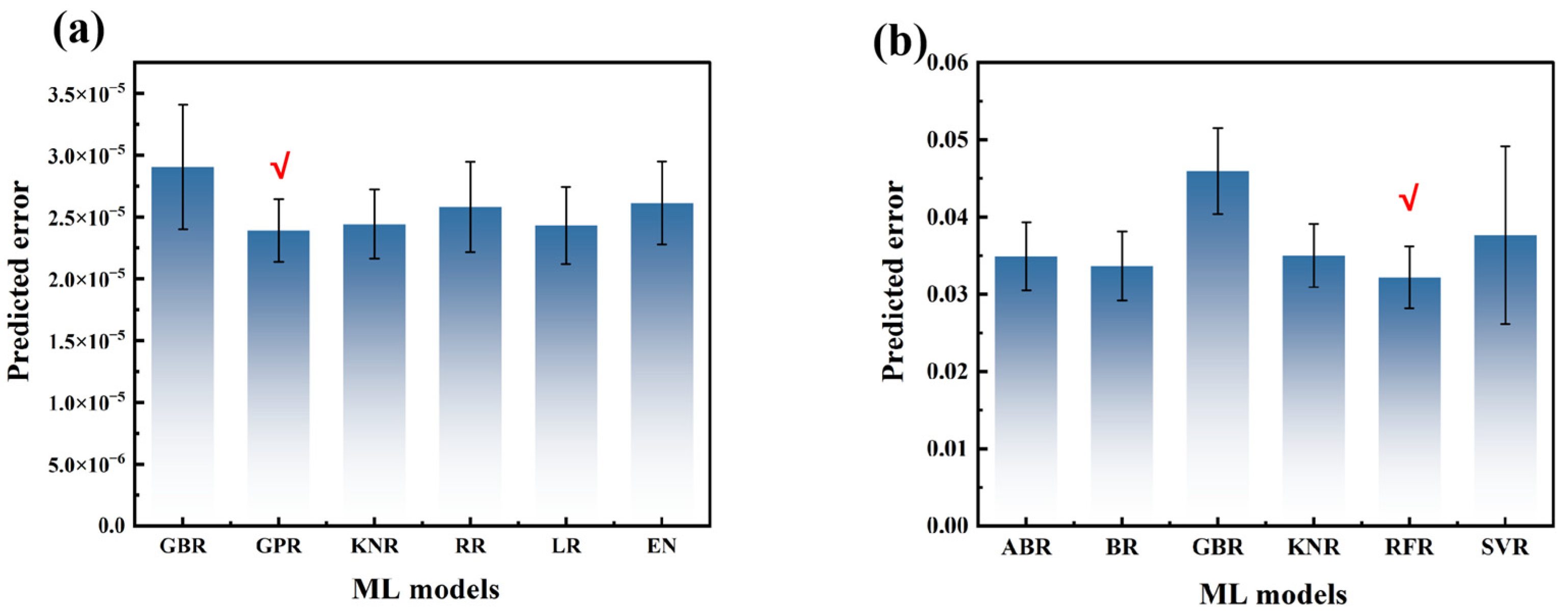
• The process was repeated 1000 times for each model with bootstrapping. After each iteration, the fine-tuning of mesh search parameters was carried out on the training set to determine the best model and parameter combination. Subsequently, the predictions were made on the test set to calculate the mean and standard deviation of the evaluation metrics, including R² and MSE. Origin, a professional drawing software recognized in the industry, and authoritative tools in the field of statistical testing, such as SciPy library in R and Python, were mainly adopted for statistical analysis and chart drawing in this study. In addition, the Matplotlib library was also used to assist in the drawing of charts.

For a given materials problem, we develop a systematic strategy flow chart aimed at finding the optimal combination of material descriptors and machine learning models, shown as Figure 1. The strategy consists of firstly experimentally collecting initial data sets, which are built based on the composition or physicochemical properties of the elements of the material. Then, we use these data to build a regression model and refine the model through the forward–backward algorithm. Next, we use the GridSearchCV method for parameter tuning to ensure the optimal performance of the model. Finally, based on the search results of GridSearchCV, we determine the best model and parameter combination and conduct a comprehensive evaluation of the performance of the trained model. The whole process is designed to ensure that we find the strategy that best fits the combination of material descriptors and machine learning models to provide more accurate and reliable predictions of material properties.

3. Results and Discussion

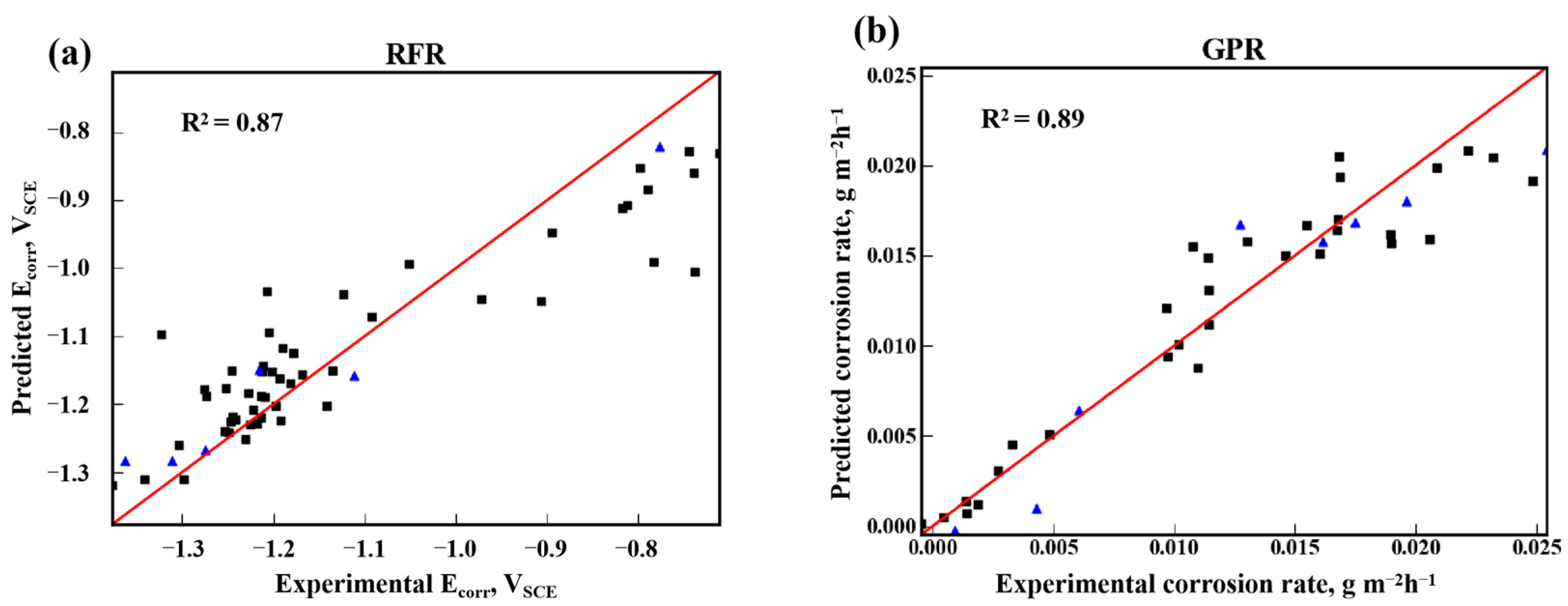
3.1. Prediction of E_corr and Corrosion Rate

The chemical compositions, corrosion rates, and E_corr values are shown in

Table 1. Corrosion data set.

Al Alloy	Composition										Ecorr	Corrosion Rate
	Al	Fe	Si	Mn	Cu	Ti	Zn	Mg	Cr	Zr	VSCE	g m−2h−1
7001	86.59	0.04	0.02	0	2.2	0	7.58	3.4	0.18	0	−0.91	0.016764943
7003	93.41	0.01	0.1	0	0	0	5.53	0.8	0	0.15	−1.3	−0.000462364
7004	93.34	0.02	0.01	0.43	0	0	4.2	1.86	0	0.13	−1.36	0.001860988
7008	93.81	0.05	0.01	0	0.09	0	4.61	1.24	0.02	0.17	−1.27	−0.000466587
7010	88.94	0.2	0.11	0.01	1.81	0.01	6.2	2.57	0.01	0.14	−1.19	0.017504447
7020	91.91	0.52	0.44	0.48	0.22	0	4.67	1.42	0.34	0	−1.14	0.011413508
7021	93.17	0.01	0.01	0	0	0	5.21	1.6	0	0	−1.34	0.001402624
7034	84.76	0.18	0.09	0.01	1	0	11.12	2.67	0	0.17	−1.21	0.020883803
7049	87.97	0.21	0.11	0.01	1.65	0.01	7.21	2.71	0.12	0	−1.22	0.016025025
7049A	87.97	0.02	0.01	0	1.59	0	7.64	2.64	0.13	0	−1.21	0.009662373
7055	85.97	0.32	0.18	0.07	2.88	0.04	8.32	1.98	0.05	0.2	−0.97	0.012719807
7065	88.39	0.21	0.1	0.01	2.2	0.01	7.1	1.79	0	0.18	−1.2	0.019599506
7075	90.31	0.09	0.03	0	1.59	0	5.13	2.64	0.2	0	−0.79	0.018946766
7076	89.08	0.06	0.03	0.5	0.82	0	7.68	1.83	0	0	−1.14	0.010975013
7085	88.42	0.08	0.04	0	1.87	0	7.76	1.71	0	0.12	−1.22	0.013017443
7108	93.14	0.07	0.02	0	0.01	0	5.29	1.25	0	0.21	−1.23	0.004287823
7150	88.89	0.05	0.03	0	2.44	0	6.08	2.42	0	0.09	−1.12	0.020571823
7175	89.94	0.1	0.06	0.01	1.73	0	5.39	2.63	0.14	0	−0.8	0.015501338
7255	86.8	0.07	0.04	0	2.5	0	8.2	2.21	0	0.18	−1.21	0.022177866
7A01	98.75	0.18	0.05	0	0.04	0	0.98	0	0	0	−0.78	0.000929177
7A02	97.36	0.03	0.01	0	0.2	0.08	1.6	0.63	0.08	0	−1.05	0.000460826
7A04	89.68	0.01	0.01	0.36	1.76	0	5.73	2.33	0.13	0	−0.74	0.016159255
7A05	91.22	0.48	0.3	0.39	0.26	0.05	5.29	1.81	0.04	0.16	−1.11	0.010170653
7A09	90.38	0.03	0.01	0.04	1.75	0	4.95	2.65	0	0.19	−0.78	0.018981165
7A10	91.58	0.02	0.01	0.28	0.77	0	3.59	3.63	0.12	0	−0.81	0.006033941
7A11	97.03	0.07	0.02	1.19	0.12	0	1.56	0	0	0	−0.82	0.00138087
7A33	92.25	0.07	0.02	0.01	0.39	0	4.76	2.43	0.07	0	−1.25	0.003284987
7A36	86.72	0.06	0.03	0.01	2.24	0	8.57	2.23	0	0.15	−1.23	0.028420891
7A46	91.64	0	0.01	0	0.27	0	6.56	1.51	0	0	−1.28	0.00272138
7A55	87.31	0.04	0.02	0.01	2.24	0.03	7.83	2.41	0	0.12	−1.21	0.024831672
7A56	87.03	0.04	0.03	0.01	1.78	0	8.83	2.12	0	0.16	−1.23	0.023217957
7A85	88.63	0.02	0.01	0	1.78	0	7.52	1.91	0.01	0.13	−1.24	0.011437292
7A88	90.9	0.06	0.03	0.41	1.45	0	4.84	2.19	0.11	0	−0.9	0.011410403
7A93	85.97	0.04	0.02	0	1.97	0	9.46	2.32	0	0.22	−1.25	0.016879487
7A99	87.96	0.03	0.01	0	1.84	0	7.66	2.35	0	0.15	−1.25	0.014618998
7B04	88.98	0.12	0.01	0.44	1.94	0	5.73	2.64	0.14	0	−0.74	0.010751195
7B68	86.98	0.02	0.01	0	2.44	0.03	7.91	2.4	0	0.21	−1.21	0.016831389
7B85	85.77	0.24	0.12	0.01	1.53	0.01	8.38	2.24	0	1.7	−1.17	0.016737208
7C04	91.92	0.01	0.01	0.4	1.79	0	3.54	2.2	0.15	0	−0.71	0.009723648
7E49	88.45	0.04	0.02	0.3	0.67	0	7.42	2.81	0	0.14	−1.25	0.004823047

. In order to reduce computation time and improve model robustness by removing the irrelevant and redundant features, we employed a hybrid method combining correlation analysis and feature selection. First, of the highly correlated features, we retained only one to reduce redundant information in the subsequent modeling. Figure 2a shows the Pearson correlation coefficient map between different features. Those with a correlation coefficient greater than 0.95 were considered highly correlated. We adopted electrochemical knowledge and the forward–backward algorithm to select the feature to be retained, and the algorithm was also used to rank the importance of each feature [32,33]. The results are shown in Figure 2b,d. The cross-validation errors of the 16 models (LR, BR, EN, LA, PAR, RR, SGDR, GPR, KNR, KRR, MLP, SVR, ABR, DTR, GBR, and RFR) based on different subsets of features were calculated. RFR showed the best performance in the prediction model of E_corr with the features of Cu, Ti, Al, and Zn, while GPR showed the best performance in the prediction model of the corrosion rate with the features of specific heat (C), latent heat of fusion (Hf1), and proportion of p electrons (P1). The test errors presented in Figure 2c,e represent the averages of the error estimates. The red boundary denotes the optimal model for a specific number of features and the optimal subset of features associated with that model. As illustrated in the figure, an increase in the number of features initially led to a decrease in the error of the machine learning model, indicating an enhancement in model performance. However, with a further increase in the number of features, the model error tended to either increase or stabilize. This observation suggests that the model error remains relatively constant or slightly increases as additional features are incorporated. When maintaining the data set size constant, an increase in the number of features does not necessarily enhance model performance but may result in overfitting [10].

Taking the best feature subset as input, the cross-validation and bootstrap methods were used to evaluate the performance of the six regression models selected by the forward–backward algorithm. The performance of the two experimental groups is presented in Figure 3. For Group I, in Figure 3a, the RFR model exhibited superior performance in predicting the corrosion potential of aluminum alloys based on compositional inputs. Conversely, for Group II, in Figure 3b, the GPR model demonstrated the best performance in predicting the corrosion rate of aluminum alloys by using atomic and physical properties as inputs.

The quality of our model predictions is shown in Figure 4, which compares the predicted and experimental values from the training data and our experimental data. The scatter points are distributed around the diagonal line, indicating that the model is adequate and the agreement is reasonable. The R² values and MSEs of the training and test groups of the two prediction models are shown in

Table 2. R² values and MSEs of the predication models of E_corr and corrosion rate.

	R2 of Training Set	R2 of Test Set	MSE of Training Set	MSE of Test Set
Ecorr	0.91	0.87	3.21 × 10−3	4.8 × 10−3
Corrosion rate	0.91	0.89	5.12 × 10−6	6.64 × 10−6

.

3.2. Characterization of Corrosion Morphology

In all the 40 specimens of 7XXX aluminum alloy, we randomly chose two specimens with high corrosion rates (7a56 and 7010, with 2.32 × 10⁻² and 1.75 × 10⁻² g m⁻²h⁻¹, respectively) and two specimens with low corrosion rates (7108 and 7003, with 4.29 × 10⁻³ and 4.62 × 10⁻⁴ g m⁻²h⁻¹, respectively) to perform microscope morphology analysis by SEM. As shown in Figure 5a,b, the high-corrosion-rate 7a56 and 7010 specimens showed a corrosion morphology featuring the precipitated phases distributed at the grain boundaries. EDS characterized a precipitated phase in the 7a56 specimen, as shown in Figure 5. It can be seen that the precipitated phase was rich in Cu, Zn, Mg, C, and O. The segregation of these elements at the grain boundaries affects the formation of precipitated phases [7]. Here, the precipitated phases and the matrix formed corrosive galvanic cells, and the latter acted as an anode during the corrosion reaction and preferential corrosion. Regarding the corrosion morphology of the low-corrosion-rate 7108 and 7003 specimens, the scratches caused by the sandpaper can be observed in Figure 5c,d, and a few corrosion pits can be seen. The degree of corrosion of the 7108 and 7003 specimens is significantly smaller than that of the 7a56 and 7010 specimens.

The features of the prediction model of E_corr mentioned in Section 3.1 were Cu, Ti, Al, and Zn, among which Cu, Al, and Zn were observed in the precipitated phase shown in Figure 6b. This means that the change in the content of these alloying elements can influence their segregation and then affect the formation and distribution of the precipitated phases in aluminum alloys, finally affecting E_corr. The features of the prediction model of the corrosion rates were specific heat (C), latent heat of fusion (Hf1), and proportion of p electrons (P1). The first two features are strongly associated with the casting process of aluminum alloy, while the last feature is related to the outermost electrons of the aluminum atom, which participate in the charge transfer process during the corrosion reaction. Thus, the two models built in this work have a physical meaning to some extent, and the machine learning method combined with the experiments can explain the corrosion mechanism in both the casting and corrosion processes.

4. Conclusions

By combining machine learning and experiments, we can predict the corrosion behavior of 7XXX Al alloys. RFR was used for the prediction model of Ecorr with the features Cu, Ti, Al, and Zn, and GPR for that of the corrosion rate with the features of specific heat, latent heat of fusion, and proportion of p electrons. Cu, Al, and Zn were observed in the precipitated phase in the 7a56 alloy. This means that the change in the composition of the precipitated phases affects E_corr. Among the features in the prediction model of the corrosion rate, specific heat and latent heat of fusion are strongly associated with the casting process of Al alloy, and the proportion of p electrons is related to the aluminum atom’s outermost electrons, which participate in the charge transfer process during the corrosion reaction.

References

1. Gest, R.J.; Troiano, A.R. Stress Corrosion and Hydrogen Embrittlement in an Aluminum Alloy. Corrosion 2013, 30, 274–279. [Google Scholar] [CrossRef]
2. Rao, A.C.U.; Vasu, V.; Govindaraju, M.; Srinadh, K.V.S. Stress corrosion cracking behaviour of 7xxx aluminum alloys: A literature review. Trans. Nonferrous Met. Soc. China 2016, 26, 1447–1471. [Google Scholar] [CrossRef]
3. Meng, S.; Yu, Y.; Zhang, X.; Zhou, L.; Liang, X.; Liu, P. Investigations on electrochemical corrosion behavior of 7075 aluminum alloy with femtosecond laser modification. Vacuum 2024, 221, 112911. [Google Scholar] [CrossRef]
4. Ji, Y.; Dong, C.; Chen, L.; Xiao, K.; Li, X. High-throughput computing for screening the potential alloying elements of a 7xxx aluminum alloy for increasing the alloy resistance to stress corrosion cracking. Corros. Sci. 2021, 183, 109304. [Google Scholar] [CrossRef]
5. Rout, P.K.; Ghosh, M.M.; Ghosh, K.S. Effect of solution pH on electrochemical and stress corrosion cracking behaviour of a 7150 Al–Zn–Mg–Cu alloy. Mater. Sci. Eng. A 2014, 604, 156–165. [Google Scholar] [CrossRef]
6. Staley, J.T. Aging kinetics of aluminum alloy 7050. Metall. Trans. 1974, 5, 929–932. [Google Scholar] [CrossRef]
7. Xue, D.; Balachandran, P.V.; Hogden, J.; Theiler, J.; Xue, D.; Lookman, T. Accelerated search for materials with targeted properties by adaptive design. Nat. Commun. 2016, 7, 11241. [Google Scholar] [CrossRef]
8. Wen, C.; Zhang, Y.; Wang, C.; Xue, D.; Bai, Y.; Antonov, S.; Dai, L.; Lookman, T.; Su, Y. Machine learning assisted design of high entropy alloys with desired property. Acta Mater. 2019, 170, 109–117. [Google Scholar] [CrossRef]
9. Stanev, V.; Oses, C.; Kusne, A.G.; Rodriguez, E.; Paglione, J.; Curtarolo, S.; Takeuchi, I. Machine learning modeling of superconducting critical temperature. Npj Comput. Mater. 2018, 4, 29. [Google Scholar] [CrossRef]
10. Wen, C.; Wang, C.; Zhang, Y.; Antonov, S.; Xue, D.; Lookman, T.; Su, Y. Modeling solid solution strengthening in high entropy alloys using machine learning. Acta Mater. 2021, 212, 116917. [Google Scholar] [CrossRef]
11. Xue, D.; Xue, D.; Yuan, R.; Zhou, Y.; Balachandran, P.V.; Ding, X.; Sun, J.; Lookman, T. An informatics approach to transformation temperatures of NiTi-based shape memory alloys. Acta Mater. 2017, 125, 532–541. [Google Scholar] [CrossRef]
12. Wei, X.; Fu, D.; Chen, M.; Wu, W.; Wu, D.; Liu, C. Data mining to effect of key alloying elements on corrosion resistance of low alloy steels in Sanya seawater environmentAlloying Elements. J. Mater. Sci. Technol. 2021, 64, 222–232. [Google Scholar] [CrossRef]
13. Lv, Y.-J.; Wang, J.-W.; Wang, J.; Xiong, C.; Zou, L.; Li, L.; Li, D.-W. Steel corrosion prediction based on support vector machines. Chaos Solitons Fractals 2020, 136, 109807. [Google Scholar] [CrossRef]
14. Liu, M.; Li, W. Prediction and analysis of corrosion rate of 3C steel using interpretable machine learning methods. Mater. Today Commun. 2023, 35, 106408. [Google Scholar] [CrossRef]
15. Feng, X.; Wang, Z.; Jiang, L.; Zhao, F.; Zhang, Z. Simultaneous enhancement in mechanical and corrosion properties of Al-Mg-Si alloys using machine learning. J. Mater. Sci. Technol. 2023, 167, 1–13. [Google Scholar] [CrossRef]
16. Ao, M.; Ji, Y.; Sun, X.; Guo, F.; Xiao, K.; Dong, C. Image Deep Learning Assisted Prediction of Mechanical and Corrosion Behavior for Al-Zn-Mg Alloys. IEEE Access 2022, 10, 35620–35631. [Google Scholar] [CrossRef]
17. Messina, J.; Luo, R.; Xu, K.; Lu, G.; Deng, H.; Tschopp, M.A.; Gao, F. Machine learning to predict aluminum segregation to magnesium grain boundaries. Scr. Mater. 2021, 204, 114150. [Google Scholar] [CrossRef]
18. Ji, Y.; Li, N.; Cheng, Z.; Fu, X.; Ao, M.; Li, M.; Sun, X.; Chowwanonthapunya, T.; Zhang, D.; Xiao, K.; et al. Random forest incorporating ab-initio calculations for corrosion rate prediction with small sample Al alloys data. Npj Mater. Degrad. 2022, 6, 83. [Google Scholar] [CrossRef]
19. Takara, Y.; Ozawa, T.; Yamaguchi, M. Analysis of the elemental effects on the surface potential of aluminum alloy using machine learning. Jpn. J. Appl. Phys. 2022, 61, SL1008. [Google Scholar] [CrossRef]
20. Blanc, C.; Mankowski, G. Susceptibility to pitting corrosion of 6056 aluminium alloy. Corros. Sci. 1997, 39, 949–959. [Google Scholar] [CrossRef]
21. Zaid, B.; Saidi, D.; Benzaid, A.; Hadji, S. Effects of pH and chloride concentration on pitting corrosion of AA6061 aluminum alloy. Corros. Sci. 2008, 50, 1841–1847. [Google Scholar] [CrossRef]
22. Blanc, C.; Lavelle, B.; Mankowski, G. The role of precipitates enriched with copper on the susceptibility to pitting corrosion of the 2024 aluminium alloy. Corros. Sci. 1997, 39, 495–510. [Google Scholar] [CrossRef]
23. ASTM G1-03; Standard Practice for Preparing, Cleaning, and Evaluating Corrosion Test Specimens. American Society of Testing Materials: West Conshohocken, PA, USA, 2017.
24. Pattanayak, S.; Dey, S.; Chatterjee, S.; Chowdhury, S.G.; Datta, S. Computational intelligence based designing of microalloyed pipeline steel. Comput. Mater. Sci. 2015, 104, 60–68. [Google Scholar] [CrossRef]
25. Jiang, L.; Wang, C.; Fu, H.; Shen, J.; Zhang, Z.; Xie, J. Discovery of aluminum alloys with ultra-strength and high-toughness via a property-oriented design strategy. J. Mater. Sci. Technol. 2022, 98, 33–43. [Google Scholar] [CrossRef]
26. Zhang, H.; Fu, H.; He, X.; Wang, C.; Jiang, L.; Chen, L.-Q.; Xie, J. Dramatically Enhanced Combination of Ultimate Tensile Strength and Electric Conductivity of Alloys via Machine Learning Screening. Acta Mater. 2020, 200, 803–810. [Google Scholar] [CrossRef]
27. Qu, Z.; Tang, D.; Wang, Z.; Li, X.; Chen, H.; Lv, Y. Pitting Judgment Model Based on Machine Learning and Feature Optimization Methods. Front. Mater. 2021, 8, 733813. [Google Scholar] [CrossRef]
28. Diao, Y.; Yan, L.; Gao, K. Improvement of the machine learning-based corrosion rate prediction model through the optimization of input features. Mater. Des. 2021, 198, 109326. [Google Scholar] [CrossRef]
29. Xie, J.; Su, Y.; Xue, D.; Jiang, X.; Fu, H.; Hung, H. Machine Learning for Materials Research and Development. Acta Metall. Sinca 2021, 57, 1343–1361. [Google Scholar]
30. Kang, Q.; Mi, X.; Wang, H.; Wu, L.; Sun, K.; Tang, A. Research Progress of Artificial Neural Networks in Material Science. Mater. Rep. 2020, 34, 11. [Google Scholar]
31. Saber, D.; Taha, I.B.M.; El-Aziz, K.A. Prediction of the Corrosion Rate of Al-Si Alloys Using Optimal Regression Methods. Intell. Autom. Soft Comput. 2021, 29, 757–769. [Google Scholar] [CrossRef]
32. Honysz, R. Modeling the Chemical Composition of Ferritic Stainless Steels with the Use of Artificial Neural Networks. Metals 2021, 11, 724. [Google Scholar] [CrossRef]
33. Churyumov, A.Y.; Kazakova, A.A. Prediction of True Stress at Hot Deformation of High Manganese Steel by Artificial Neural Network Modeling. Materials 2023, 16, 1083. [Google Scholar] [CrossRef]
Figure 1. Flow diagram for this work.
Metals 14 00401 g001
Figure 2. (a) Pearson correlation analysis results for Group II. The feature matrix is jointly listed on both the horizontal and vertical axes, while the color band on the right side of the figure depicts the correlation coefficients. Blue and red colors signify positive and negative correlations, respectively. Lighter tones indicate less significant correlations. The filled portion of each pie chart corresponds to the absolute value of the associated Pearson correlation coefficient. A deeper color indicates a high level of correlation. (b,d) Ranking by importance of the compositions (Group I) and physical features (Group II), respectively. The importance ranking is determined by using the BackForward module, which records the frequency of feature selection in the model throughout the entire process. This statistical approach effectively captures the significance and stability of each feature, ultimately leading to the identification of the most critical ones. (c,e) Optimal feature subset obtained through feature selection, where Group I included Cu, Ti, Al, and Zn, and Group II, C, Hf1, and P1. After thoroughly examining all conceivable combinations of features and utilizing cross-validation to evaluate the model’s performance on each distinct feature subset, we identified the most effective subset of features. In (c,e), the red dash frontier tracks the best model for various features. The green dot indicates the set of features employed in the cross-validation. In (b,c), the machine learning process of the prediction model of Ecorr is shown, and in (a,d,e), that of the corrosion rate is shown.
Metals 14 00401 g002
Figure 3. Evaluation of models by using bootstrap method. (a) Ecorr, (b) corrosion rate. The red checkmark indicates the optimal algorithm.
Metals 14 00401 g003
Figure 4. The predicted versus measured values for the Al alloys of the training and test sets of the prediction model of Ecorr (a) and corrosion rate (b), respectively. The black square points are the training set, and the blue triangle points are the test set.
Metals 14 00401 g004
Figure 5. The micromorphology of the Al alloy specimens after the immersion test and the removal of the corrosion products. (a) 7a56, (b) 7010, (c) 7108, and (d) 7003.
Metals 14 00401 g005
Figure 6. EDS results of precipitated phase in 7a56 specimen. (a) micromorphology of the precipitated phase, (b) The chemical composition of the precipitated phase.
Metals 14 00401 g006