
Experimental Investigation of Stress Concentration and Fatigue Behavior in 9% Ni Steel Welded Joints under Cryogenic Conditions

Abstract
:1. Introduction
2. Butt-Welded Specimens’ SCF Prediction
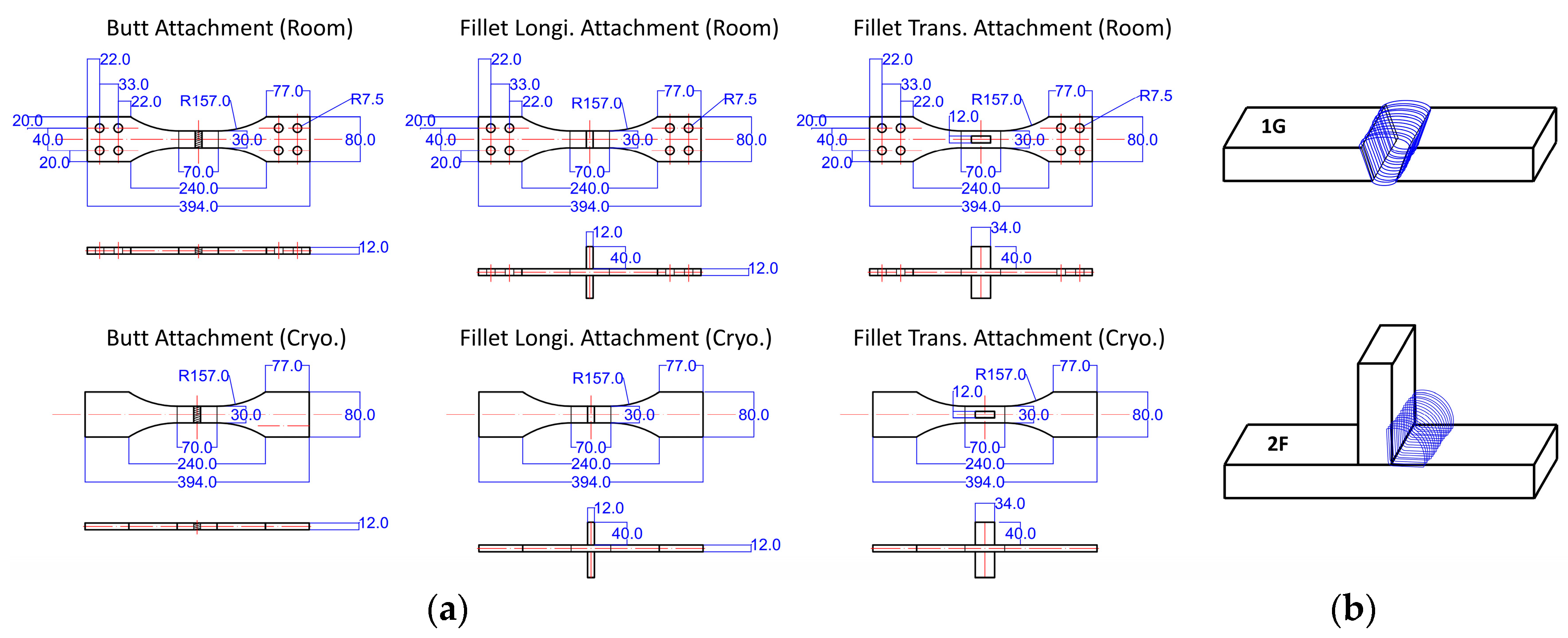
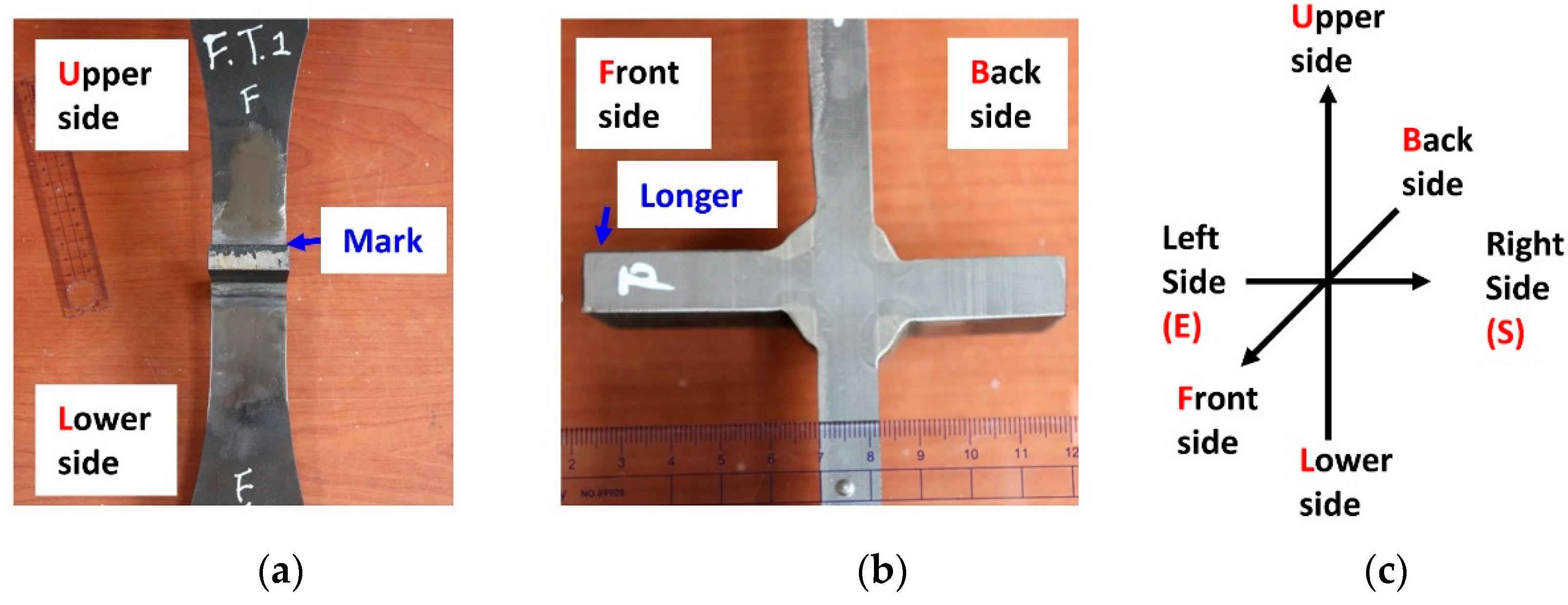
2.1. Orientation and Measurement
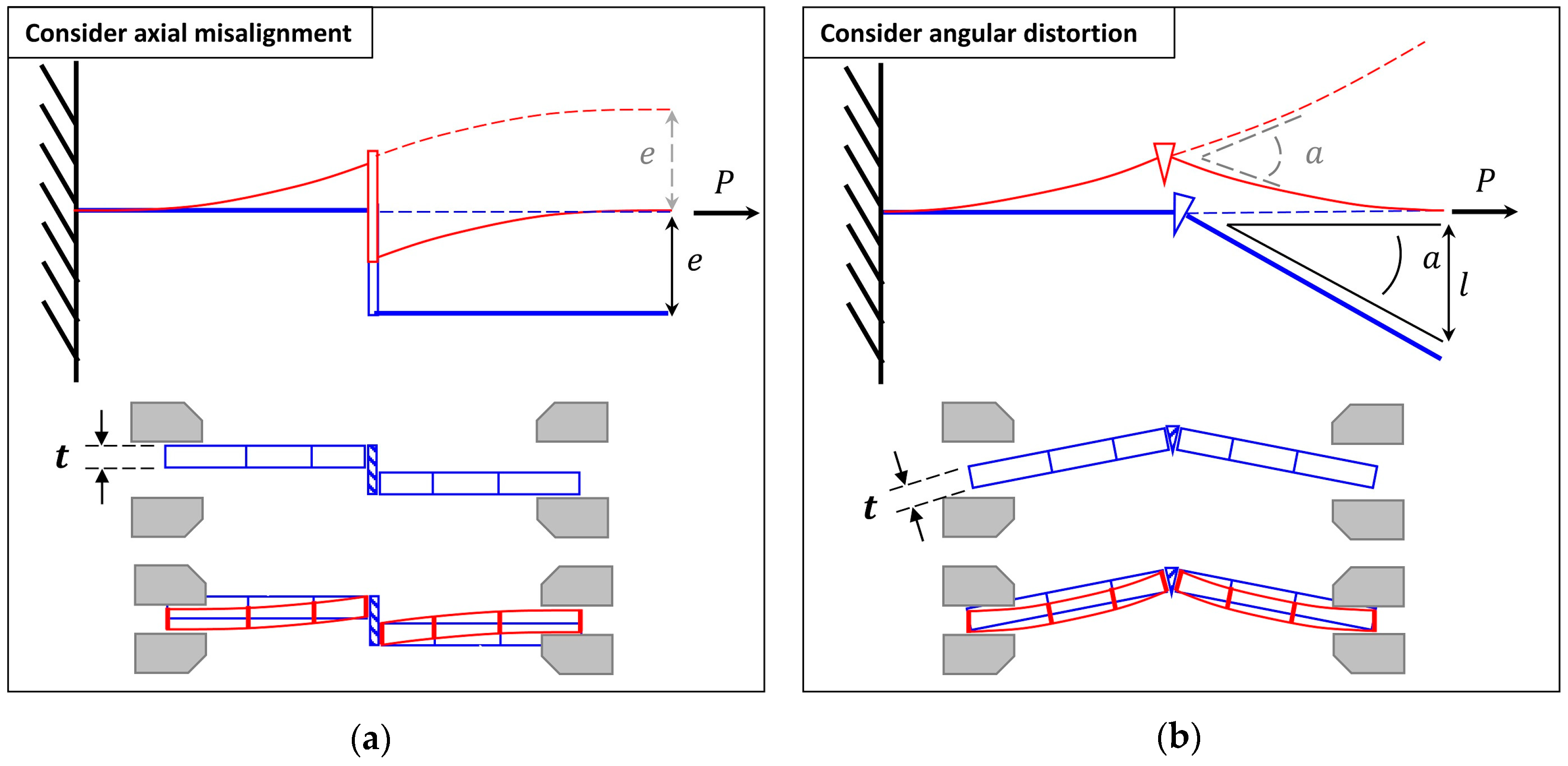
2.2. SCF Prediction Method Review
- : the stress magnification factor due to axial misalignment (dimensionless);
- : the stress magnification factor due to angular distortion (dimensionless);
- : 3 for clamped; 6 for pinned condition;
- : the total length of the specimen (mm);
- : the thickness of the specimen (mm).
2.3. Stress Components
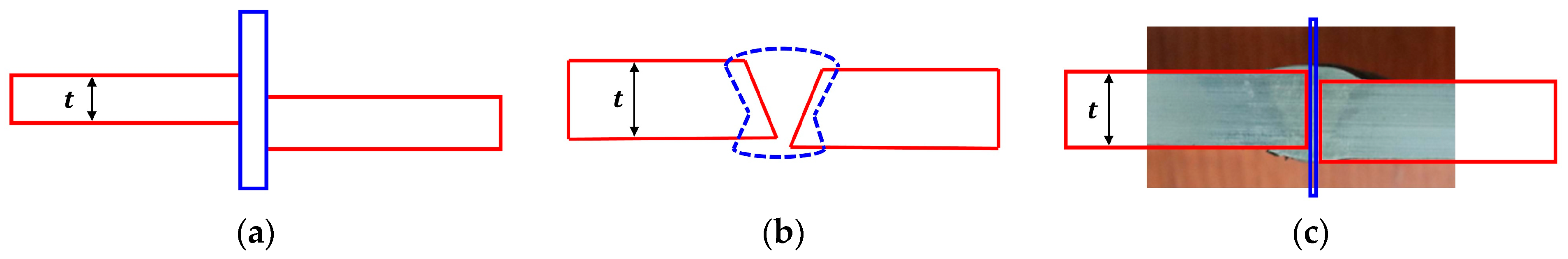
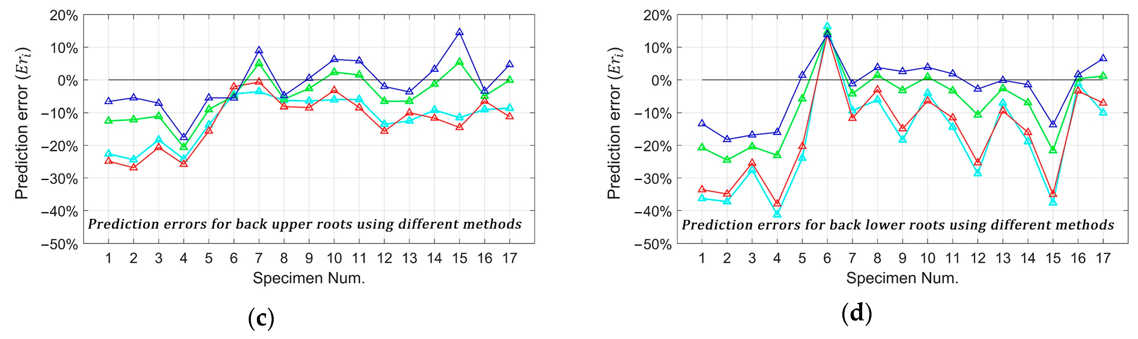
2.4. The Bead Effect
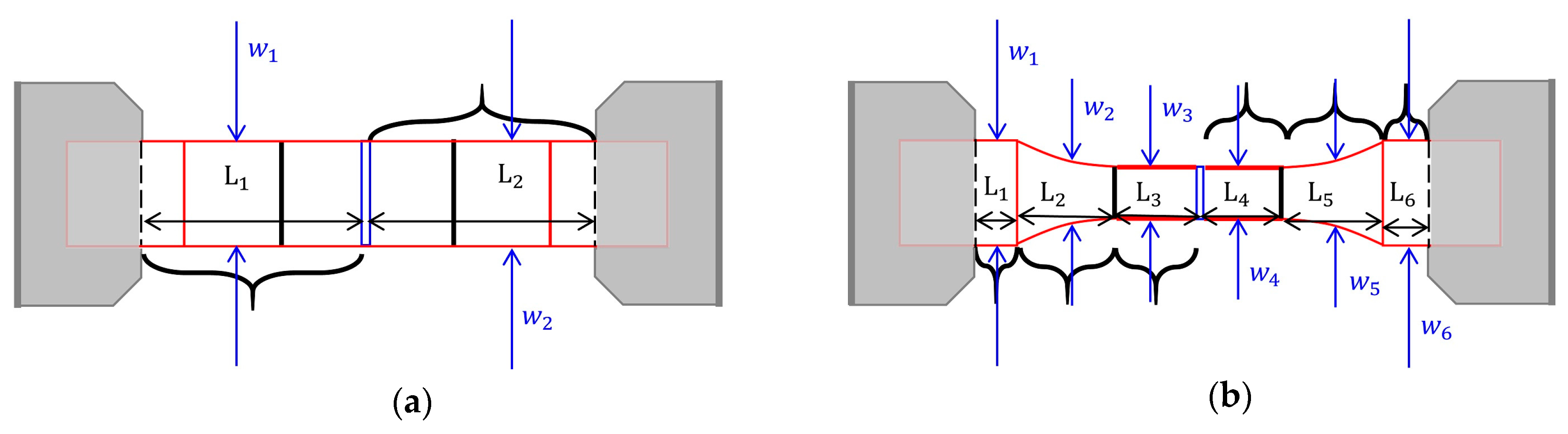
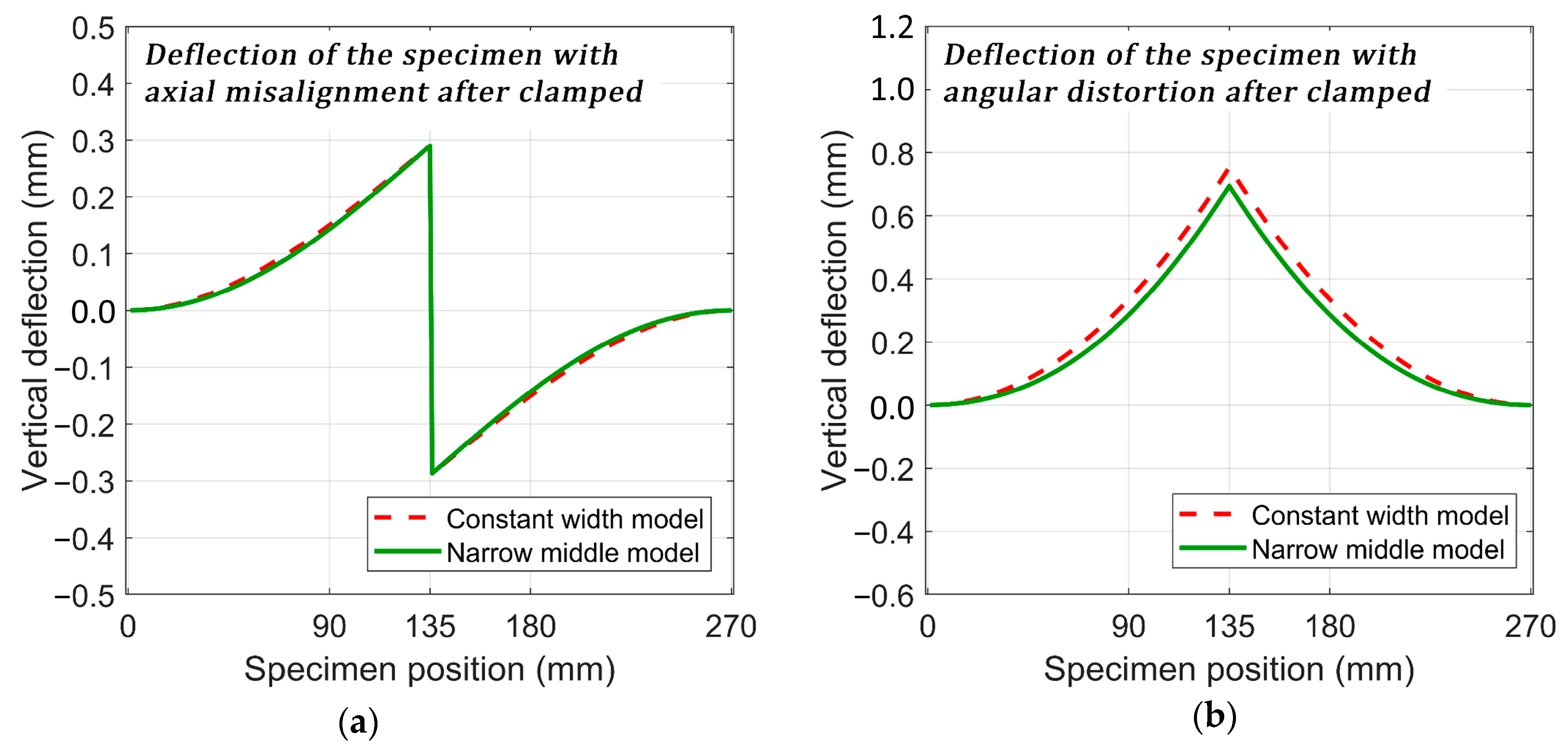
2.5. The Clamped and Reduced Mid-Section Effect
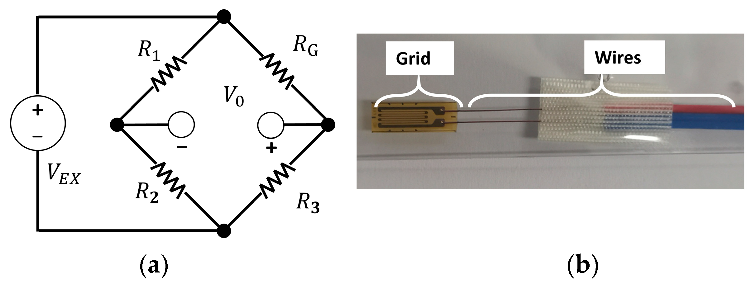
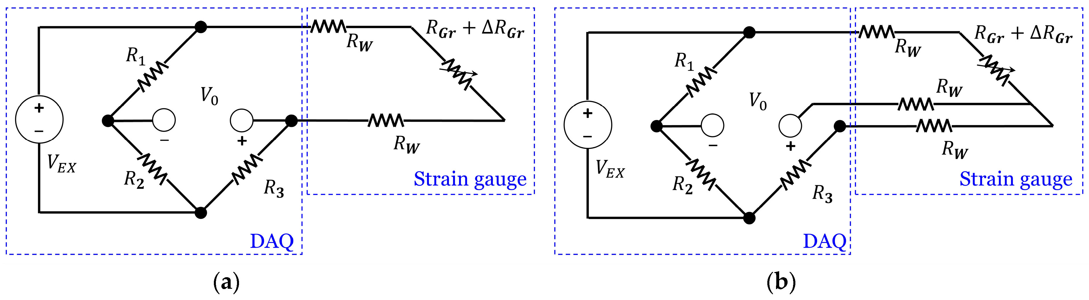
3. Calibrating the 2-Wire Strain Gauge Output
4. Fatigue Test and Test Results
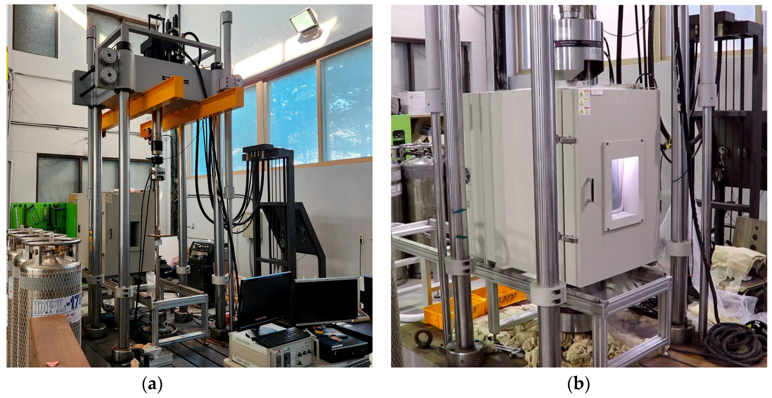
4.1. Test Introduction
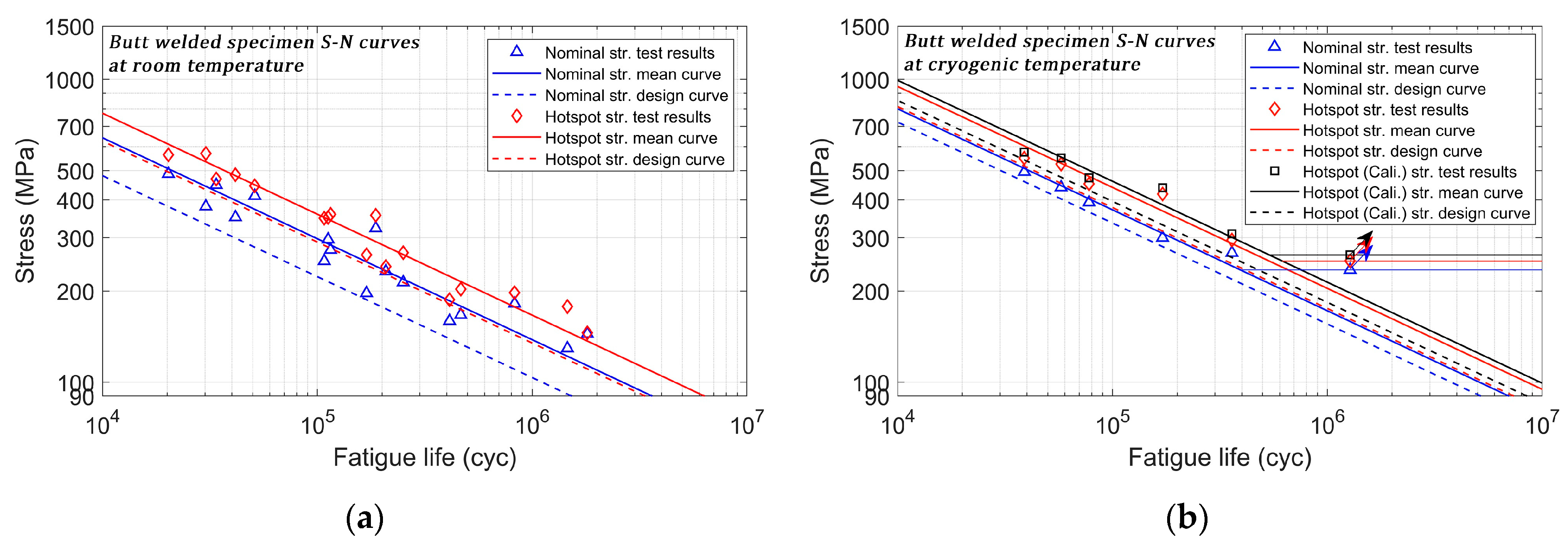
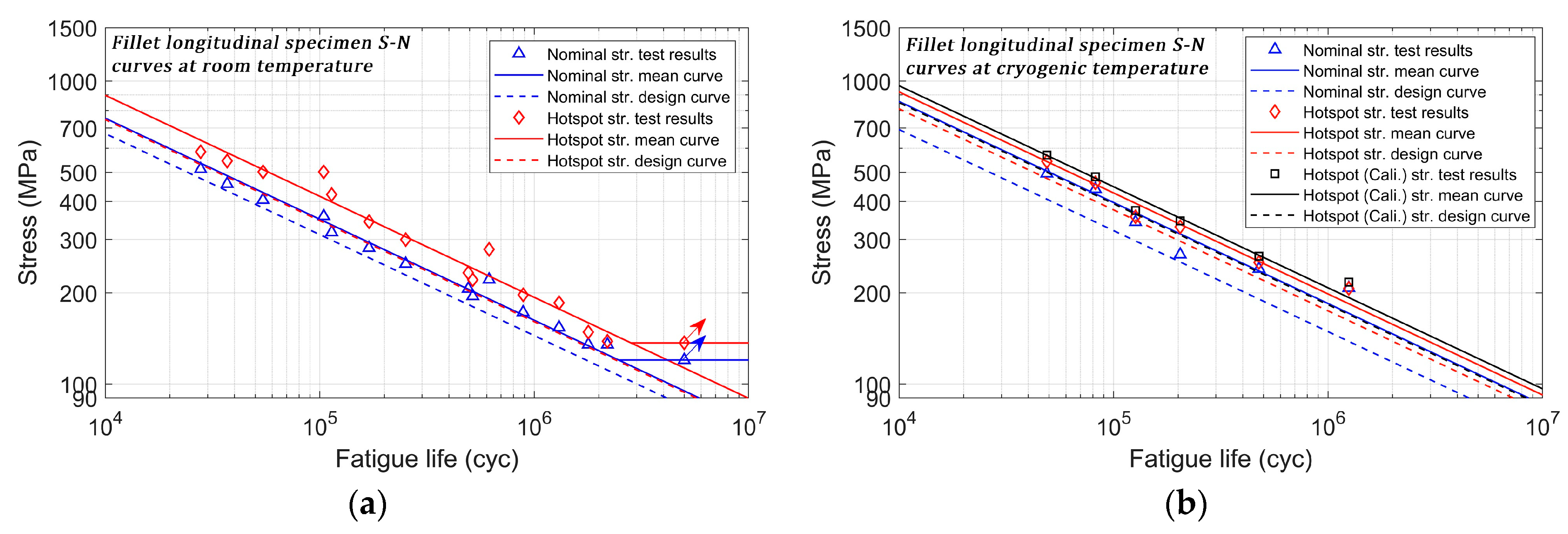
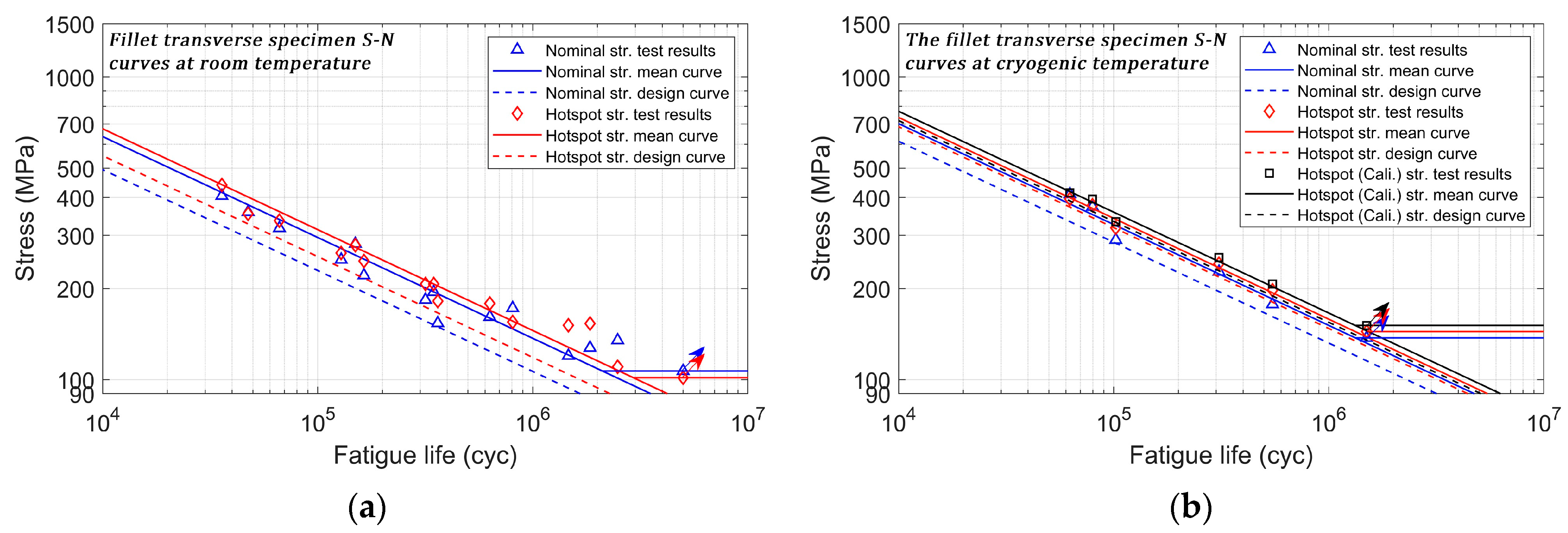
4.2. S-N Curve
4.3. Fracture Point
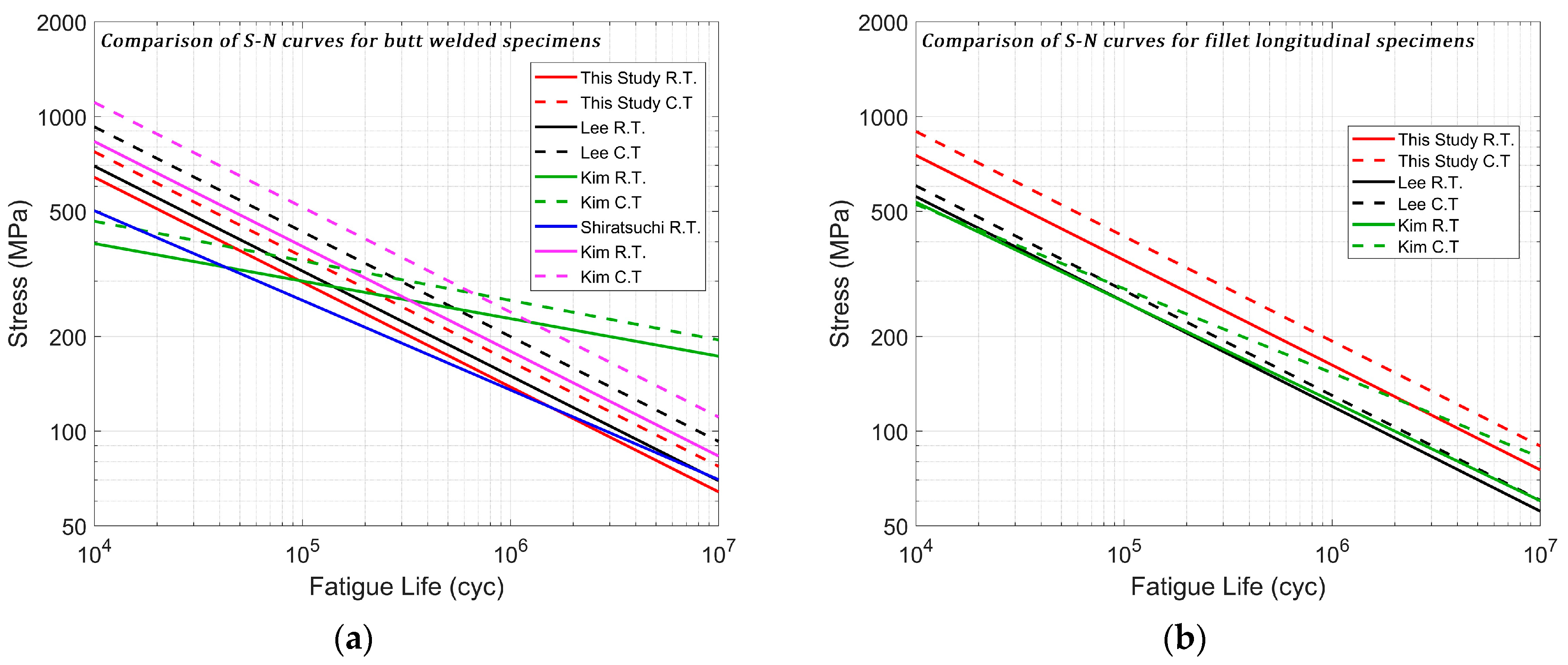
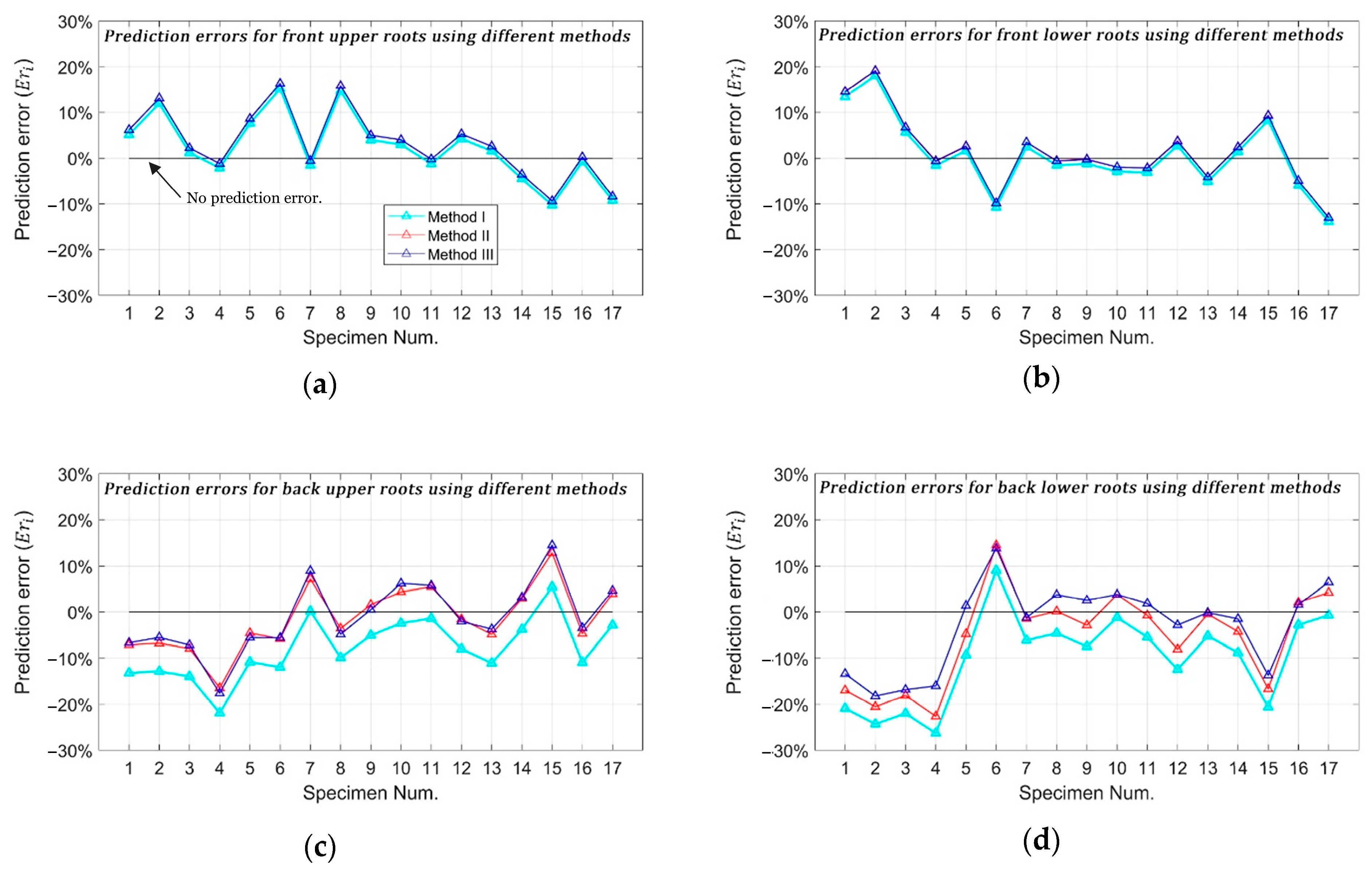
4.4. Comparison of the S-N Curve
5. Discussion of Butt-Welded Test Results
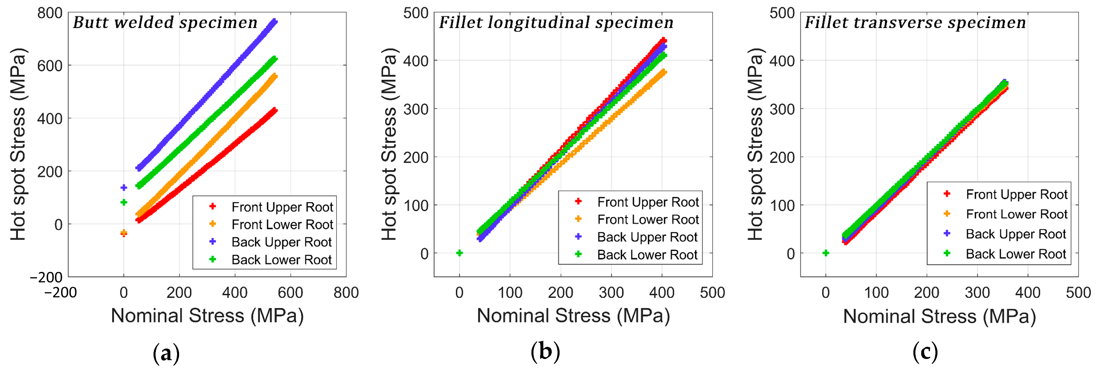
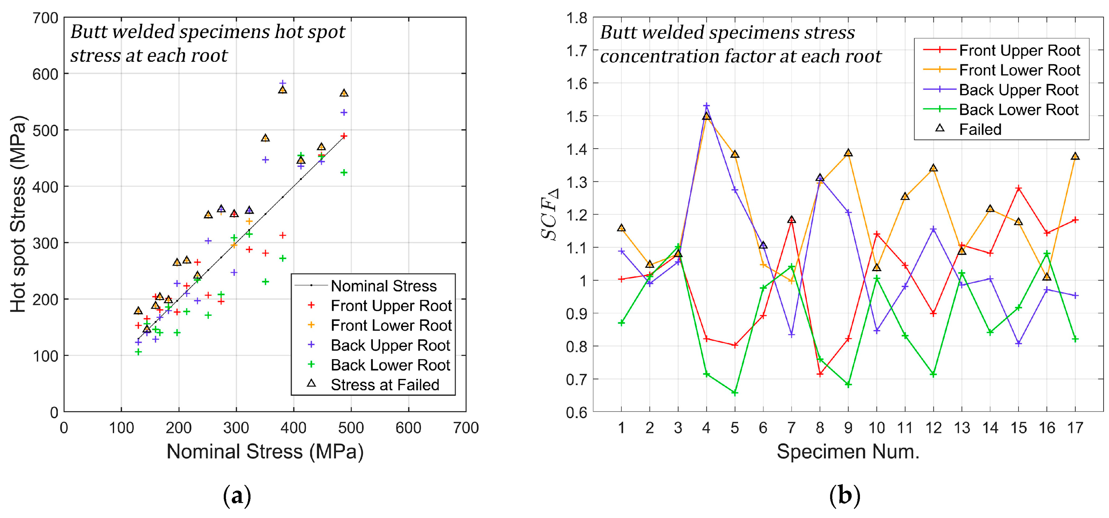
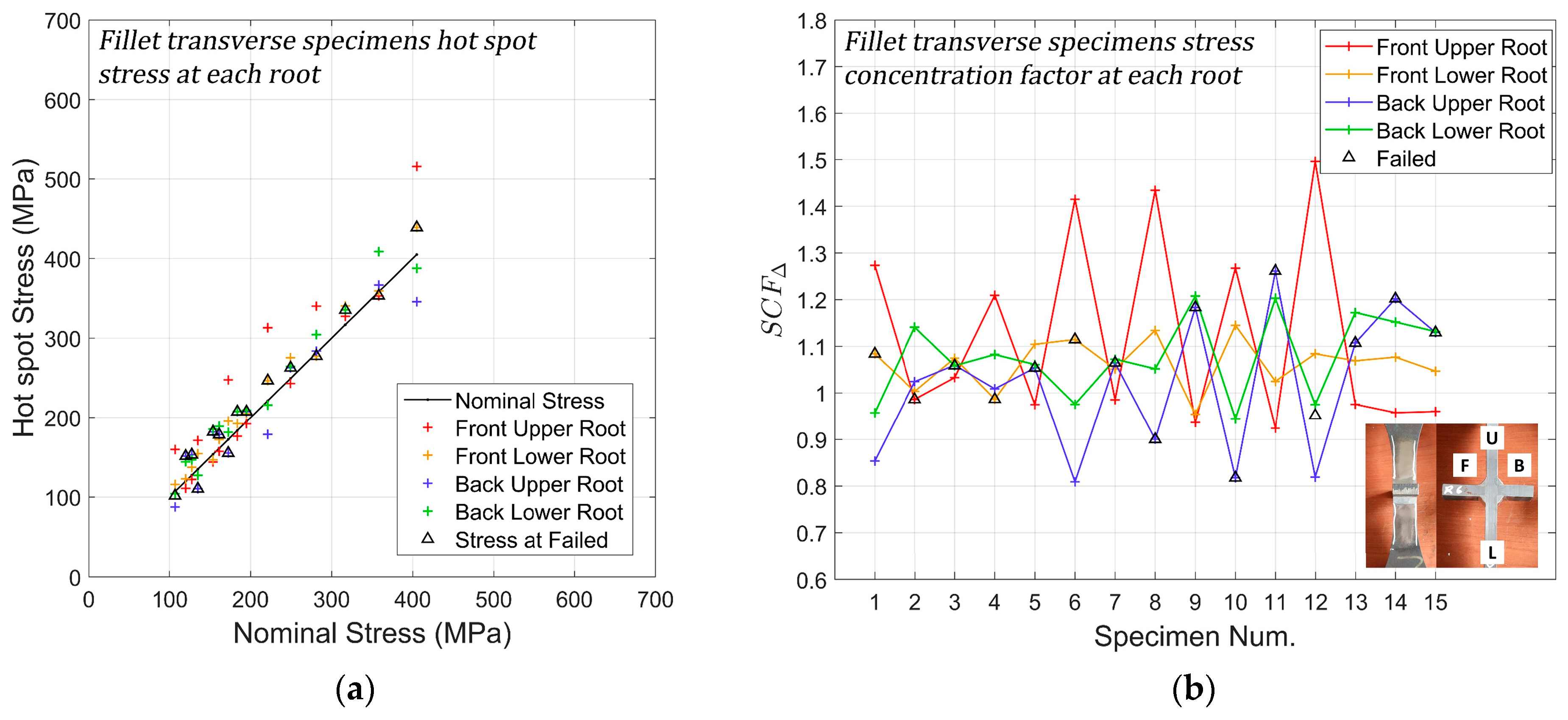
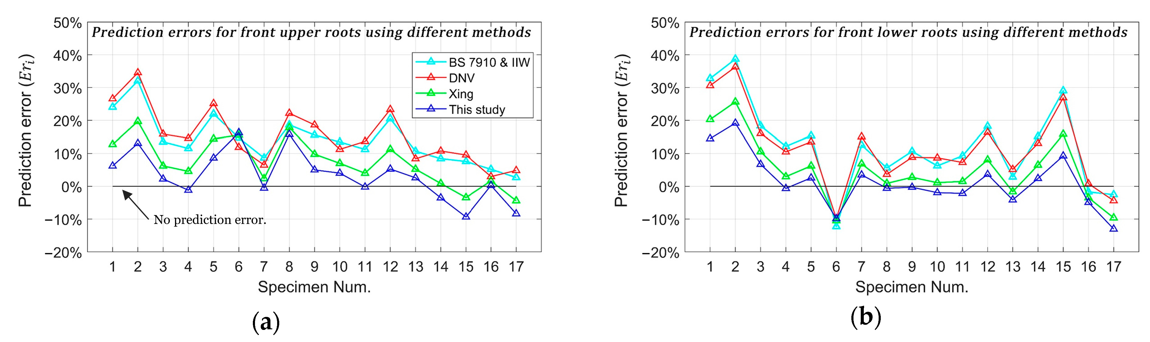
5.1. Hot-Spot Stress Prediction
- : from prediction;
- : from the test result;
- : specimen number.
5.2. Predicted Hot-Spot Stress-Based S-N Curve
6. Conclusions
- To address potential issues during strain gauge measurements, the study proposes a hot-spot stress prediction method. This method considers multiple factors influencing hot-spot stress, enhancing the reliability of stress predictions. Experimental verification confirms the accuracy of predicted hot-spot stresses compared to measured values.
- This study proposes an innovative approach focusing on the influence of the mid-section of the specimen on stress concentration factor (SCF) prediction. Taking into account the clamped effect and the reduced mid-section allows the obtained , values to more accurately predict the hot-spot stress.
- The bead is found to have different effects on the axial tensile stress and on the bending stress concentration. By considering the effect of the bead on axial nominal stress and on bending stress separately, the prediction accuracy can also be improved.
- The research discovers that the ratio of output strain between 3-wire and 2-wire strain gauges remains constant. This finding allows for the correction of 2-wire strain gauge outputs in cryogenic environments, thereby improving the accuracy of experimental results.
Author Contributions
Funding
Data Availability Statement
Acknowledgments
Conflicts of Interest
Abbreviations
| Average of prediction errors of all specimens at each root | |
| Average of prediction errors of all specimens from four roots | |
| prediction error for specimen | |
| The corresponding stress on the curve when fatigue life (cycles) | |
| Gauge factor | |
| 2-/3-wire strain gauge factor in room/cryogenic temperature | |
| / | The total length of the specimen/length of each part of the specimen |
| Mean curve | |
| Design curve | |
| 2-/3-wire strain gauge grid resistance | |
| Gauge resistance | |
| Gauge grid resistance | |
| Gauge wire resistance | |
| Stress concentration factor | |
| Stress concentration factor when focusing on the loading range | |
| from prediction | |
| from the test | |
| / | Fatigue life curve parameters |
| Axial misalignment | |
| The axial misalignment used to calculate in DNV | |
| Stress magnification factor due to angular distortion | |
| Stress magnification factor due to the bead from axial tensile/bending FE model | |
| Stress magnification factor due to the bead | |
| Stress magnification factor due to the bead from bending FE model | |
| Stress magnification factor due to axial misalignment | |
| Correlation coefficient | |
| Standard deviation | |
| Thickness | |
| / | Width of the specimen/width of each part of the specimen |
| Change in resistance of the gauge grid due to deformation of attached object | |
| Hot-spot stress range | |
| Hot-spot stress range from the test after calibration | |
| Hot-spot stress range from prediction | |
| Hot-spot stress range from the test | |
| Nominal stress for balanced axial load in specimen | |
| Bending stress range due to misalignment | |
| Bending stresses for balanced moment in angular distortion existed specimen | |
| Bending stresses for balanced moment in axial misalignment existed specimen | |
| Nominal stress range | |
| Angular distortion | |
| Strain | |
| Strain measured at cryogenic temperature by the 2-wire strain gauge, if accurate/inaccurate gauge factor is used | |
| Strain measured by the 2-/3-wire strain gauge at room/cryogenic temperature | |
| Hot-spot stress | |
| Hot-spot stress obtained from the FE model when axial tensile/bending stress is applied | |
| Hot-spot stress initiated by gripping | |
| Hot-spot stress initiated by nominal stress | |
| Nominal bending stress induced by gripping | |
| Nominal stress | |
| The applied nominal axial tensile/bending stress when studying the bead effect |
Appendix A

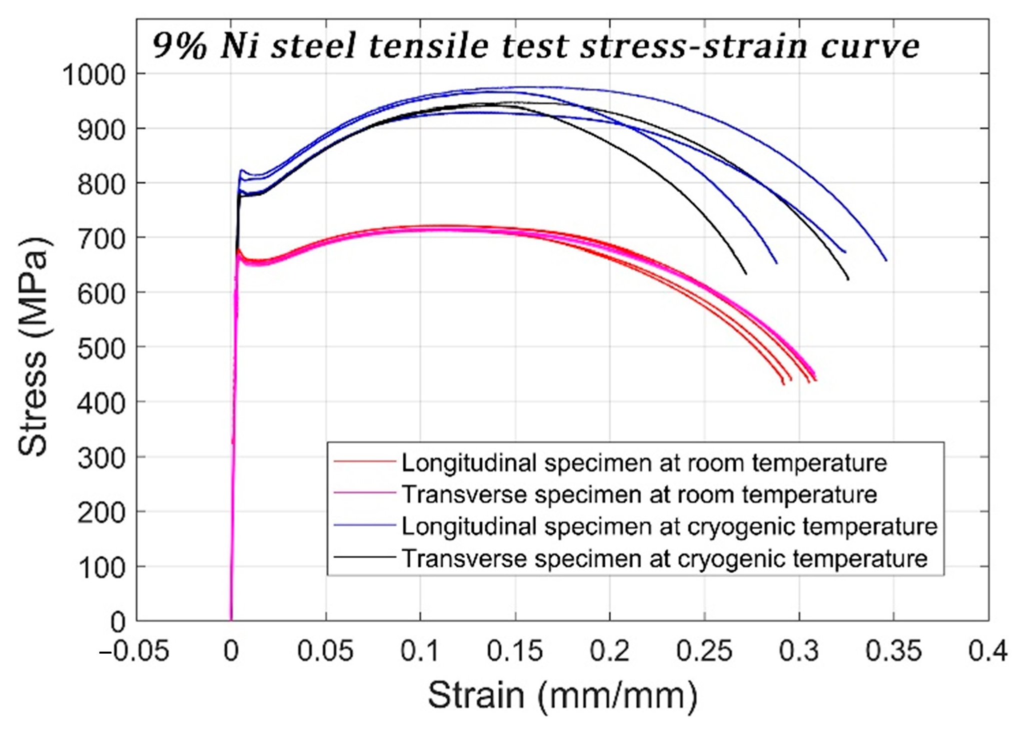
| Temperature | E (GPa) | Yield | Tensile | Fracture | |||||
|---|---|---|---|---|---|---|---|---|---|
| Upper | Lower | ||||||||
| Strength (MPa) | Strain (mm/mm) | Strength (MPa) | Strain (mm/mm) | Strength (MPa) | Strain (mm/mm) | Strength (MPa) | Strain (mm/mm) | ||
| Cryogenic ) | 204.9 | 796.9 | 0.49% | 790.2 | 0.85% | 951.4 | 14.34% | 629.6 | 31.24% |
| Room ) | 197.3 | 670.3 | 0.40% | 654.2 | 1.53% | 716.4 | 10.97% | 438.7 | 30.31% |
References
- Serindağ, H.T.; Tardu, C.; Kirçiçek, İ.Ö.; Çam, G. A study on microstructural and mechanical properties of gas tungsten arc welded thick cryogenic 9% Ni alloy steel butt joint. CIRP J. Manuf. Sci. Technol. 2022, 37, 1–10. [Google Scholar] [CrossRef]
- MEPC. Amendments to the Annex of the Protocol of 1997 to Amend the International Convention for the Prevention of Pollution From Ships, 1973, as Modified by the Protocol of 1978 Relating Thereto. In Amendments to MARPOL Annex VI; MEPC: London, UK, 2011; Volume 70, p. 18. [Google Scholar]
- Abdussamie, N.; Daboos, M.; Elferjani, I.; Shuhong, C.; Alaktiwi, A. Risk assessment of LNG and FLNG vessels during manoeuvring in open sea. J. Ocean Eng. Sci. 2018, 3, 56–66. [Google Scholar] [CrossRef]
- Cao, Y.; Jia, Q.J.; Wang, S.M.; Jiang, Y.; Bai, Y. Safety design analysis of a vent mast on a LNG powered ship during a low-temperature combustible gas leakage accident. J. Ocean Eng. Sci. 2022, 7, 75–83. [Google Scholar] [CrossRef]
- Oh, D.J.; Lee, J.M.; Noh, B.J.; Kim, W.S.; Ryuichi-Ando; Toshiyuki-Matsumoto; Kim, M.H. Investigation of fatigue performance of low temperature alloys for liquefied natural gas storage tanks. Proc. Inst. Mech. Eng. Part C-J. Eng. Mech. Eng. Sci. 2015, 229, 1300–1314. [Google Scholar] [CrossRef]
- Lee, J.S.; You, W.H.; Yoo, C.H.; Kim, K.S.; Kim, Y. An experimental study on fatigue performance of cryogenic metallic materials for IMO type B tank. Int. J. Nav. Archit. Ocean Eng. 2013, 5, 580–597. [Google Scholar] [CrossRef]
- Kim, Y.W.; Oh, D.J.; Lee, J.M.; Noh, B.J.; Sung, H.J.; Ando, R.; Matsumoto, T.; Kim, M.H. An experimental study for fatigue performance of 7% nickel steels for type b liquefied natural gas carriers. J. Offshore Mech. Arct. Eng. 2016, 138, 031401. [Google Scholar] [CrossRef]
- Shiratsuchi, T.; Osawa, N. Fatigue life prediction for 9% Ni steel butt welded joints. Int. J. Fatigue 2021, 142, 105925. [Google Scholar] [CrossRef]
- Kim, T.Y.; Yoon, S.W.; Kim, J.H.; Kim, M.H. Fatigue and Fracture Behavior of Cryogenic Materials Applied to LNG Fuel Storage Tanks for Coastal Ships. Metals 2021, 11, 1899. [Google Scholar] [CrossRef]
- Saini, D.S.; Karmakar, D.; Ray-Chaudhuri, S. A review of stress concentration factors in tubular and non-tubular joints for design of offshore installations. J. Ocean Eng. Sci. 2016, 1, 186–202. [Google Scholar] [CrossRef]
- Dong, Y.; Teixeira, A.P.; Soares, C.G. Fatigue reliability analysis of butt welded joints with misalignments based on hotspot stress approach. Mar. Struct. 2019, 65, 215–228. [Google Scholar] [CrossRef]
- Xin, H.; Correia, J.A.F.O.; Veljkovic, M.; Berto, F.; Manuel, L. Residual stress effects on fatigue life prediction using hardness measurements for butt-welded joints made of high strength steels. Int. J. Fatigue 2021, 147, 106175. [Google Scholar] [CrossRef]
- Kim, M.H.; Kim, S.M.; Kim, Y.N.; Kim, S.G.; Lee, K.E.; Kim, G.R. A comparative study for the fatigue assessment of a ship structure by use of hot spot stress and structural stress approaches. Ocean Eng. 2009, 36, 1067–1072. [Google Scholar] [CrossRef]
- Xing, S.; Dong, P. An analytical SCF solution method for joint misalignments and application in fatigue test data interpretation. Mar. Struct. 2016, 50, 143–161. [Google Scholar] [CrossRef]
- Berge, S.; Myhre, H. Fatigue strength of misaligned cruciform and butt joints. Norw. Mar. Res. 1977, 5, 29–39. [Google Scholar]
- Braun, M.; Kellner, L.; Schreiber, S.; Ehlers, S. Prediction of fatigue failure in small-scale butt-welded joints with explainable machine learning. Procedia Struct. Integr. 2022, 38, 182–191. [Google Scholar] [CrossRef]
- Chen, Z.; Yu, B.; Wang, P.; Qian, H.; Dong, P. Fatigue behaviors of aluminum alloy butt joints with backing plates: Experimental testing and traction stress modeling. Int. J. Fatigue 2022, 163, 107040. [Google Scholar] [CrossRef]
- Qiu, Y.; Shen, W.; Yan, R.; Xu, L.; Liu, E. Fatigue reliability evaluation of thin plate welded joints considering initial welding deformation. Ocean Eng. 2021, 236, 109440. [Google Scholar] [CrossRef]
- Cui, W.; Wan, Z.; Mansour, A.E. Stress concentration factor in plates with transverse butt-weld misalignment. J. Constr. Steel. Res. 1999, 52, 159–170. [Google Scholar] [CrossRef]
- Kang, S.W.; Park, Y.M.; Jang, B.S.; Jeon, Y.C.; Kim, S.M. Study on fatigue experiment for transverse butt welds under 2G and 3G weld positions. Int. J. Nav. Archit. Ocean Eng. 2015, 7, 833–847. [Google Scholar] [CrossRef]
- Lillemäe, I.; Lammi, H.; Molter, L.; Remes, H. Fatigue strength of welded butt joints in thin and slender specimens. Int. J. Fatigue 2012, 44, 98–106. [Google Scholar] [CrossRef]
- Mashiri, F.R.; Zhao, X.L.; Grundy, P. Effects of weld profile and undercut on fatigue crack propagation life of thin-walled cruciform joint. Thin-Walled Struct. 2001, 39, 261–285. [Google Scholar] [CrossRef]
- Hong, K.; Oterkus, S.; Oterkus, E. Peridynamic analysis of fatigue crack growth in fillet welded joints. Ocean Eng. 2021, 235, 109348. [Google Scholar] [CrossRef]
- Chen, Z.; Yu, B.; Wang, P.; Qian, H. Fatigue properties evaluation of fillet weld joints in full-scale steel marine structures. Ocean Eng. 2023, 270, 113651. [Google Scholar] [CrossRef]
- Xing, S.; Pei, X.; Mei, J.; Dong, P.; Su, S.; Zhen, C. Weld toe versus root fatigue failure mode and governing parameters: A study of aluminum alloy load-carrying fillet joints. Mar. Struct. 2023, 88, 103344. [Google Scholar] [CrossRef]
- Ahola, A.; Björk, T. Fatigue strength of misaligned non-load-carrying cruciform joints made of ultra-high-strength steel. J. Constr. Steel. Res. 2020, 175, 106334. [Google Scholar] [CrossRef]
- Skriko, T.; Ahola, A.; Poutiainen, I.; Björk, T. Fatigue strength of laser-dressed non-load-carrying fillet weld joints made of ultra-high-strength steel. Procedia Struct. Integr. 2022, 38, 393–400. [Google Scholar] [CrossRef]
- BS 7910; Guide to Methods for Assessing the Acceptability of Flaws in Metallic Structures. British Standard: London, UK, 2015. [CrossRef]
- Hobbacher, A. Recommendations for Fatigue Design of Welded Joints and Components; IIW (International Institute of Welding): Paris, France, 2018. [Google Scholar] [CrossRef]
- DNV. Fatigue design of offshore steel structures. In DNV Recommended Practice (DNV-RP-C203); DNV: Oslo, Norway, 2010. [Google Scholar]
- Shen, W.; Qiu, Y.; Xu, L.; Song, L. Stress concentration effect of thin plate joints considering welding defects. Ocean Eng. 2019, 184, 273–288. [Google Scholar] [CrossRef]
- ASTM E466; Standard Practice for Conducting Force Controlled Constant Amplitude Axial Fatigue Tests of Metallic Materials. ASTM International: West Conshohocken, PA, USA, 2015. [CrossRef]
- Hannah, R.; Reed, S.E. Strain Gage Users’ Handbook; Springer Science & Business Media: Berlin/Heidelberg, Germany, 1992. [Google Scholar]
- ASTM E8/E8M; Standard Test Methods for Tension Testing of Metallic Materials. ASTM International: West Conshohocken, PA, USA, 2014. [CrossRef]


| Author | Year | Bead Effect | Misalignment Effect | |||||
|---|---|---|---|---|---|---|---|---|
| Axial Load | Bending Component | Axial Misalignment | Angular Distortion | Misalignment Location | Clamping Effect | Reduced Middle Section | ||
| Berge and Myhre adapted from Ref. [15] | 1977 | - | - | ☑ | ☑ | - | - | - |
| Cui et al. adapted from Ref. [19] | 1999 | - | ☑ | - | ☑ | - | - | |
| Lillemäe et al. adapted from Ref. [21] | 2012 | ☑ | - | ☑ | ☑ | - | - | - |
| Kang et al. adapted from Ref. [20] | 2015 | ☑ | - | ☑ | ☑ | - | ☑ | - |
| Xing and Dong adapted from Ref. [14] | 2016 | - | - | ☑ | ☑ | ☑ | ☑ | - |
| Present study | ☑ | ☑ | ☑ | ☑ | ☑ | ☑ | ☑ | |
| Root Position | Front Upper | Front Lower | Back Upper | Back Lower |
|---|---|---|---|---|
| ) | − | + | + | − |
| ) | + | + | − | − |
| Test Item | Welding Process | Thickness (mm) | Welding Position |
|---|---|---|---|
| Butt-Welded | FCAW | 12 | 1G |
| Fillet Longitudinal | FCAW | 12 | 2F |
| Fillet Transverse | FCAW | 12 | 2F |
| Fatigue Test Results (loga Represents the Logarithm Based on e) | Butt-Welded Specimen | Fillet Longitudinal Specimen | Fillet Transverse Specimen | ||
|---|---|---|---|---|---|
| Room Temperature | Curve | 28.60 | 29.08 | 28.58 | |
| r2 | 0.8897 | 0.9841 | 0.9155 | ||
| FAT(M) | 109.7 | 128.8 | 108.8 | ||
| FAT(M-2STD) | 82.2 | 114.7 | 84.6 | ||
Curve | 29.16 | 29.61 | 28.75 | ||
| r2 | 0.9403 | 0.9600 | 0.9439 | ||
| FAT(M) | 132.2 | 153.4 | 115.4 | ||
| FAT(M-2STD) | 106.9 | 127.5 | 94.0 | ||
| Cryogenic Temperature | Curve | 29.26 | 29.47 | 28.87 | |
| r2 | 0.9642 | 0.9132 | 0.942 | ||
| FAT(M) | 136.7 | 146.4 | 120.0 | ||
| FAT(M-2STD) | 123.6 | 118.2 | 104.9 | ||
Curve | 29.77 | 29.68 | 29.01 | ||
| r2 | 0.9174 | 0.9686 | 0.9841 | ||
| FAT(M) | 162.0 | 157.4 | 125.8 | ||
| FAT(M-2STD) | 139.0 | 138.4 | 117.3 | ||
Curve | 29.91 | 29.82 | 29.15 | ||
| r2 | 0.9174 | 0.9686 | 0.9841 | ||
| FAT(M) | 169.8 | 164.5 | 131.9 | ||
| FAT(M-2STD) | 145.7 | 145.0 | 122.9 | ||
| Author | Parameters (Mean Curve) | Butt-Welded | Fillet Longitudinal | Fillet Transverse | Thickness (mm) | Stress Ratio | |
|---|---|---|---|---|---|---|---|
| Room Temperature | This Study | 28.60 | 29.08 | 28.58 | 12 | 0.1 | |
| 3 | 3 | 3 | |||||
| FAT | 109.7 | 128.8 | 108.8 | ||||
| Lee et al. Adapted from Ref. [6] | 28.85 | 28.18 | / | 12 | 0 | ||
| 3 | 3 | / | |||||
| FAT | 119.0 | 95.2 | / | ||||
| Kim et al. Adapted from Ref. [7] | 59.31 | 29.06 | / | 12 | 0 | ||
| 8.38 | 3.16 | / | |||||
| FAT | 209.8 | 100.0 | / | ||||
| Shiratsuchi and Osawa Adapted from Ref. [8] | 31.01 | / | / | 22 | 0.05 | ||
| 3.51 | / | / | |||||
| FAT | 111.0 | / | / | ||||
| Kim et al. Adapted from Ref. [9] | 29.39 | / | / | 8 | 0.1 | ||
| 3 | / | / | |||||
| FAT | 142.5 | / | / | ||||
| Cryogenic Temperature | This Study | 29.26 | 29.47 | 28.87 | 12 | 0.1 | |
| 3 | 3 | 3 | |||||
| FAT | 132.2 | 153.4 | 115.4 | ||||
| Lee et al. Adapted from Ref. [6] | 29.18 | 28.42 | / | 12 | 0 | ||
| 3 | 3 | / | |||||
| FAT | 158.6 | 103.1 | / | ||||
| Kim et al. Adapted from Ref. [7] | 58.03 | 32.58 | / | 12 | 0 | ||
| 7.95 | 3.73 | / | |||||
| FAT | 238.8 | 127.1 | / | ||||
| Kim et al. Adapted from Ref. [9] | 30.24 | / | / | 8 | 0.1 | ||
| 3 | / | / | |||||
| FAT | 189.7 | / | / |
| Author | Contents | ||
|---|---|---|---|
| BS 7910 Adapted from Ref. [29] and IIW Adapted from Ref. [30] | Classical method | 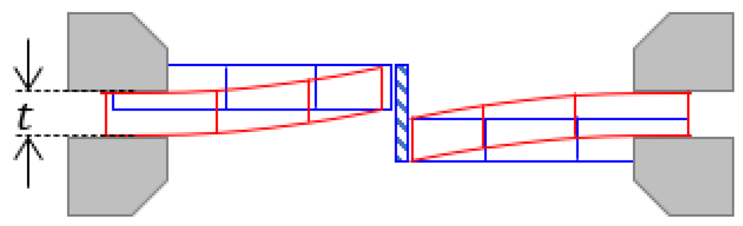 |  |
| DNV Adapted from Ref. [31] | Misalignment Tolerance | 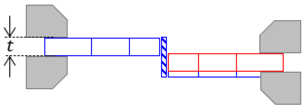 | 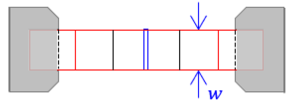 |
| Xing and Dong Adapted from Ref. [14] | Clamped effect |  |  |
| This study | Clamped effect andNarrow mid-section |  | 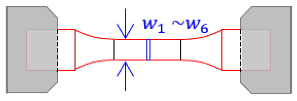 |
| Method | Contents | ||
|---|---|---|---|
| Value Selection | Value Selection | Formula | |
| Method I | |||
| Method II | |||
| Method III | |||
| FU | FL | BU | BL | Average | |
|---|---|---|---|---|---|
| BS 7910 and IIW | 14.15% | 14.32% | 11.79% | 19.91% | 15.04% |
| DNV | 15.34% | 13.35% | 12.62% | 18.23% | 14.89% |
| 8.30% | 7.90% | 6.63% | 9.73% | 8.14% | |
| This Study | 6.03% | 5.84% | 6.23% | 7.01% | 6.28% |
| Number of crack occurrences | 2/17 | 13/17 | 2/17 | 0/17 | /S |
| FU | FL | BU | BL | Average | |
|---|---|---|---|---|---|
| Method I | 5.77% | 5.85% | 8.57% | 11.01% | 7.80% |
| Method II | 6.03% | 5.85% | 5.98% | 8.36% | 6.56% |
| Method III | 6.03% | 5.84% | 6.23% | 7.01% | 6.28% |
| Number of crack occurrences | 2/17 | 13/17 | 2/17 | 0/17 | / |
| Different Ways to Consider the Bead Effect | Average | ||||
|---|---|---|---|---|---|
| Method I | Method II | Method III | |||
| Different methods to calculate the and | BS 7910 and IIW | 18.18% | 16.48% | 15.04% | 16.32% |
| DNV | 18.45% | 16.78% | 14.89% | 16.49% | |
| 10.69% | 8.84% | 8.14% | 9.02% | ||
| This Study | 7.80% | 6.56% | 6.28% | 6.75% | |
| Average | 13.78% | 12.16% | 11.09% | - | |
| Butt-Welded Specimen | Room Temperature | Cryogenic Temperature | ||
|---|---|---|---|---|
| Nominal stress based | 28.60 | 29.26 | ||
| 0.8897 | 0.9642 | |||
| FAT | 109.7 (MPa) | 136.7 (MPa) | ||
| Hot-spot stress-based (from the test) | 29.16 | 29.77 | ||
| 0.9403 | 0.9174 | |||
| FAT | 132.2 (MPa) | 162.0 (MPa) | ||
| Hot-spot stress-based (from test and calibration) | / | 29.91 | ||
| / | 0.9174 | |||
| FAT | / | 169.8 (MPa) | ||
| Hot-spot stress-based (from prediction) | 29.18 | 29.74 | ||
| 0.9719 | 0.9765 | |||
| FAT | 133.0 (MPa) | 160.4 (MPa) | ||
Disclaimer/Publisher’s Note: The statements, opinions and data contained in all publications are solely those of the individual author(s) and contributor(s) and not of MDPI and/or the editor(s). MDPI and/or the editor(s) disclaim responsibility for any injury to people or property resulting from any ideas, methods, instructions or products referred to in the content. |
© 2024 by the authors. Licensee MDPI, Basel, Switzerland. This article is an open access article distributed under the terms and conditions of the Creative Commons Attribution (CC BY) license (https://creativecommons.org/licenses/by/4.0/).
Share and Cite
Lin, Y.-Y.; Han, S.-W.; Park, Y.-H.; Kim, D.K. Experimental Investigation of Stress Concentration and Fatigue Behavior in 9% Ni Steel Welded Joints under Cryogenic Conditions. Metals 2024, 14, 741. https://doi.org/10.3390/met14070741
Lin Y-Y, Han S-W, Park Y-H, Kim DK. Experimental Investigation of Stress Concentration and Fatigue Behavior in 9% Ni Steel Welded Joints under Cryogenic Conditions. Metals. 2024; 14(7):741. https://doi.org/10.3390/met14070741
Chicago/Turabian StyleLin, Yu-Yao, Sang-Woong Han, Young-Hwan Park, and Do Kyun Kim. 2024. "Experimental Investigation of Stress Concentration and Fatigue Behavior in 9% Ni Steel Welded Joints under Cryogenic Conditions" Metals 14, no. 7: 741. https://doi.org/10.3390/met14070741