Multi-Output Prediction Model for Basic Oxygen Furnace Steelmaking Based on the Fusion of Deep Convolution and Attention Mechanisms

Abstract

The objective of basic oxygen furnace (BOF) steelmaking is to achieve molten steel with final carbon content, temperature, and phosphorus content meeting the requirements. Accurate prediction of the above properties is crucial for end-point control in BOF steelmaking. Traditional prediction models typically use multi-variable input and single-variable output approaches, neglecting the coupling relationships between different property indicators, making it difficult to predict multiple outputs simultaneously. Consequently, a multi-output prediction model based on the fusion of deep convolution and attention mechanism networks (FDCAN) is proposed. The model inputs include scalar data, such as the properties of raw materials and target molten steel, and time series data, such as lance height, oxygen supply intensity, and bottom air supply intensity during the blowing process. The FDCAN model utilizes a fully connected module to extract nonlinear features from scalar data and a deep convolution module to process time series data, capturing high-dimensional feature representations. The attention mechanism then assigns greater weight to significant features. Finally, multiple multi-layer perceptron modules predict the outputs—final carbon content, temperature, and phosphorus content. This structure allows FDCAN to learn complex relationships within the input data and between input and output variables. The effectiveness of the FDCAN model is validated using actual BOF steelmaking data, achieving hit rates of 95.14% for final carbon content within ±0.015 wt%, 84.72% for final temperature within ±15 °C, and 88.89% for final phosphorus content within ±0.005 wt%.

1. Introduction

Basic oxygen furnace (BOF) steelmaking is the most widely employed method worldwide. In recent years, due to the continuous development of intelligent manufacturing technology in the metallurgical field, end-point control technology in BOF steelmaking has evolved towards automatic control driven by intelligent models [1,2]. The final carbon content, phosphorus content, and temperature of molten steel are keys to the endpoint control of BOF steelmaking. Inadequate control of carbon content increases the nitrogen and oxygen levels in the steel while excessive carbon content hampers the dephosphorization and desulfurization processes in molten steel. In other words, inadequate or excessive carbon content reduces the properties of steel [3]. Similarly, an excessively high or low final temperature will also increase the consumption of coolant and auxiliary materials, which not only prolongs the converting time but also has a great impact on the life of the furnace lining [4]. The increase in phosphorus content in steel will significantly reduce the strength and toughness of the steel, resulting in increased cold brittleness [5]. Hence, the precise prediction of final carbon content, phosphorus content, and temperature in molten steel can effectively reduce production costs, shorten the steelmaking cycle, stabilize control of the steelmaking process, and improve the properties of molten steel.

Traditional end-point prediction models for BOF steelmaking primarily consist of mechanism-based models and intelligent models [6,7]. For different steel grades in different steel plants, BOF steelmaking has varying requirements for the accuracy of the final carbon and phosphorus contents and the temperature of the molten steel [8]. The allowable error ranges [9,10] are typically within ±0.005 wt%, ±0.010 wt%, ±0.015 wt%, or ±0.020 wt% for carbon content; within ±10 °C, ±15 °C, or ±20 °C for temperature; and within ±0.003 wt%, ±0.005 wt%, or ±0.007 wt% for phosphorus content. Based on these standards, the existing mechanism-based models and intelligent models can meet these requirements to varying degrees.

Mechanism-based models are established on principles derived from reaction mechanisms, including mass balance, heat balance, thermodynamics, fluid flow [11], and mass transport coefficients. Some scholars have utilized mechanism-based models to predict the final carbon content, temperature, and phosphorus content of BOF steelmaking. For instance, Schlautmann et al. [12] developed a dynamic model for the final phosphorus content in BOF steelmaking based on detailed investigations regarding the related thermodynamics, fluid flow, and kinetics by mass transport. Feng et al. [13] proposed a case-based reasoning method based on mechanistic model similarity (CBR-MM). This method utilizes the slag phosphorus distribution ratio and the principle of conservation of matter to predict the final phosphorus content. Li et al. [14] introduced the concept of molten pool mixing degree based on traditional three-stage decarburization theory and proposed a model for the simultaneous prediction of carbon content and temperature at the end of BOF steelmaking, considering the impact of the oxygen jet on decarburization. The hit rate for final temperature within ±20 °C was 83.3%, carbon content was 82.6% within ±0.02 wt% (when below 0.1 wt%), and the double hit rate for both was 70.8%. Therefore, it can be concluded that these models’ prediction accuracies largely satisfy the practical production requirements.

In recent years, with the rapid development of computer technology, intelligent algorithms have been increasingly used in the metallurgical field. Compared with traditional mechanism models, intelligent models have obvious advantages in handling complex nonlinear relationships within data [15]. Therefore, many scholars have proposed intelligent models, such as machine learning regression prediction (MLRP) models [16,17,18] and neural network prediction (NNP) models [19,20], to improve the final prediction accuracy of BOF steelmaking. In terms of MLRP models, Han et al. [21] integrated fuzzy c-means clustering, mutual information, and support vector regression (SVR) to improve case reasoning for predicting final carbon content in BOF steelmaking. The model was validated with actual data from a 180-ton converter, and the hit rate of final carbon content reached 91.98% within ±0.02 wt%. Gao et al. [22] proposed a BOF steelmaking end-point control model using improved unconstrained twin support vector regression (IUTSVR). For the 100-heat test set, the double hit rate for carbon content within ±0.005 wt% and temperature within ±15 °C was 90%. In addition to the intelligent models based on the SVR method. Zhang et al. [23] compared five machine learning models for predicting final phosphorus content, including ridge regression, gradient boosting regression, SVR, random forest regression (RFR), and convolutional neural networks. The RFR model performed best, with a root mean square error of 0.00319 wt%. Qian et al. introduced the functional kernel partial least squares (FKPLS) method [24] and the functional relevance vector machine (FRVM) method [25]. The FKPLS method achieved mean relative prediction errors of less than 15.31% for carbon content and 0.66% for temperature in molten steel. The FRVM method had a mean relative prediction error of less than 18.09% for phosphorus content in molten steel. The above scholars validated their models using extensive production data, demonstrating good applicability and stability under various conditions.

In terms of NNP models, such methods achieve data learning and prediction by establishing a multi-layer network structure and a nonlinear activation function to automatically capture the characteristics of the data [26,27,28,29]. Improved prediction models based on deep neural networks are widely used for predicting the end point of BOF steelmaking. He et al. [30] established an intelligent model combining principal component analysis (PCA) and a back propagation neural network (BPNN) to predict the final phosphorus content. The hit rates for phosphorus content within the error range of ±0.007 wt%, ±0.005 wt%, and ±0.004 wt% were 96.67%, 93.33%, and 86.67%. Liu et al. [31] proposed a hybrid model (PCA-GA-BP) combining PCA, a genetic algorithm (GA), and a BPNN. Applied to a 250-ton BOF, the PCA–GA–BP method achieved a root mean square error of 7.89 °C for temperature and 0.0030 wt% for carbon content. Zhou et al. [32] proposed a final phosphorus content prediction model based on a monotone-constrained BPNN (MC-BP). Using actual production data, the hit rates within error ranges of ±0.005 wt% and ±0.003 wt% were 94% and 74%. Gu et al. [33] combined the CBR algorithm with a long short-term memory (LSTM) network to create a real-time prediction model for carbon content in the final stage of BOF steelmaking. The hit rates for carbon content within error ranges of ±0.015 wt% and ±0.020 wt% were 71%, and 91%. The above results show that NNP models have effectively predicted the final carbon and phosphorus contents and temperature in BOF steelmaking.

It can be seen from the results of the above prediction models that different models developed for the BOF steelmaking process led to different results. The differences in model methodologies are the primary reason for the differing prediction results. Mechanism-based models involve the modeling of physical and chemical processes, often involving numerous theoretical assumptions and complex calculations. In contrast, intelligent models are data-driven, learning from vast amounts of historical data to recognize patterns and make predictions. These two approaches handle nonlinear relationships and complex variables differently, leading to differing results. Additionally, intelligent models usually require complex feature extraction methods to improve prediction accuracy, and the choice of different feature extraction methods can lead to varying model performance. In conclusion, traditional mechanism-based models rely on numerous theoretical assumptions and struggle with the strong nonlinear relationship between the final properties of molten steel and process parameters, limiting their predictive accuracy. The MLRP models, while improving accuracy and generalization, are hindered by the complexity of feature extraction and the selection of appropriate methods. The NNP models, despite using mixed scalar and time series data, often fail to fully utilize time series information and typically focus on single-variable outputs, neglecting the coupling relationships between different property indicators. Therefore, effective feature extraction from mixed data and the decoupling of property relationships remain critical challenges.

In view of the problems existing in the traditional prediction model, a multi-output prediction model based on the fusion of deep convolution and attention mechanism networks (FDCAN) is proposed. Scalar data such as the properties of raw materials and target molten steel, as well as time series data, such as lance height, oxygen supply intensity, and bottom air supply intensity, are used as inputs to the prediction model. The FDCAN model extracts non-linear features from scalar data using a fully connected module, while a deep convolution module extracts features from time series data. Then, these features are concatenated and input into the attention-augmented multi-layer perceptron module, which assigns weights to the features. The weighted features are used to predict the final carbon and phosphorous contents and temperature of steel through three multi-layer perceptron modules. The advantages of the FDCAN method are as follows. (1) In order to extract features of mixed input variables, the fully connected module is used to extract nonlinear features of scalar data, and the embedding and group convolution modules are used to process time series data. The embedding module can map data to high channel dimensions and facilitate the extraction of long-term dependencies by slicing the time series. Two sets of group convolutions are used to extract local features of the time series in the channel and variable dimension, which is beneficial to capturing the complex temporal correlation within the blowing process parameters. (2) In order to decouple the complex relationship between different output variables, the attention mechanism is used to give greater weight to important features. Multiple independent multi-layer perceptron modules are used to learn the mapping relationship between each output variable and important features separately. The above branch structure helps capture the potential correlation between all variables and maintain the independence of the output variables. The effectiveness of the FDCAN model is verified using actual data from BOF steelmaking.

The rest of the paper is organized as follows. Section 2 describes the problems present in traditional end-point property prediction models and gives a brief overview of the principle of multi-output property prediction models. Section 3 details the FDCAN model architecture. Section 4 verifies the model’s effectiveness using BOF steelmaking data, discusses core parameters, and selects optimal values for the best predictions. Comparison methods and ablation experiments further validate the FDCAN model. Section 5 concludes the paper.

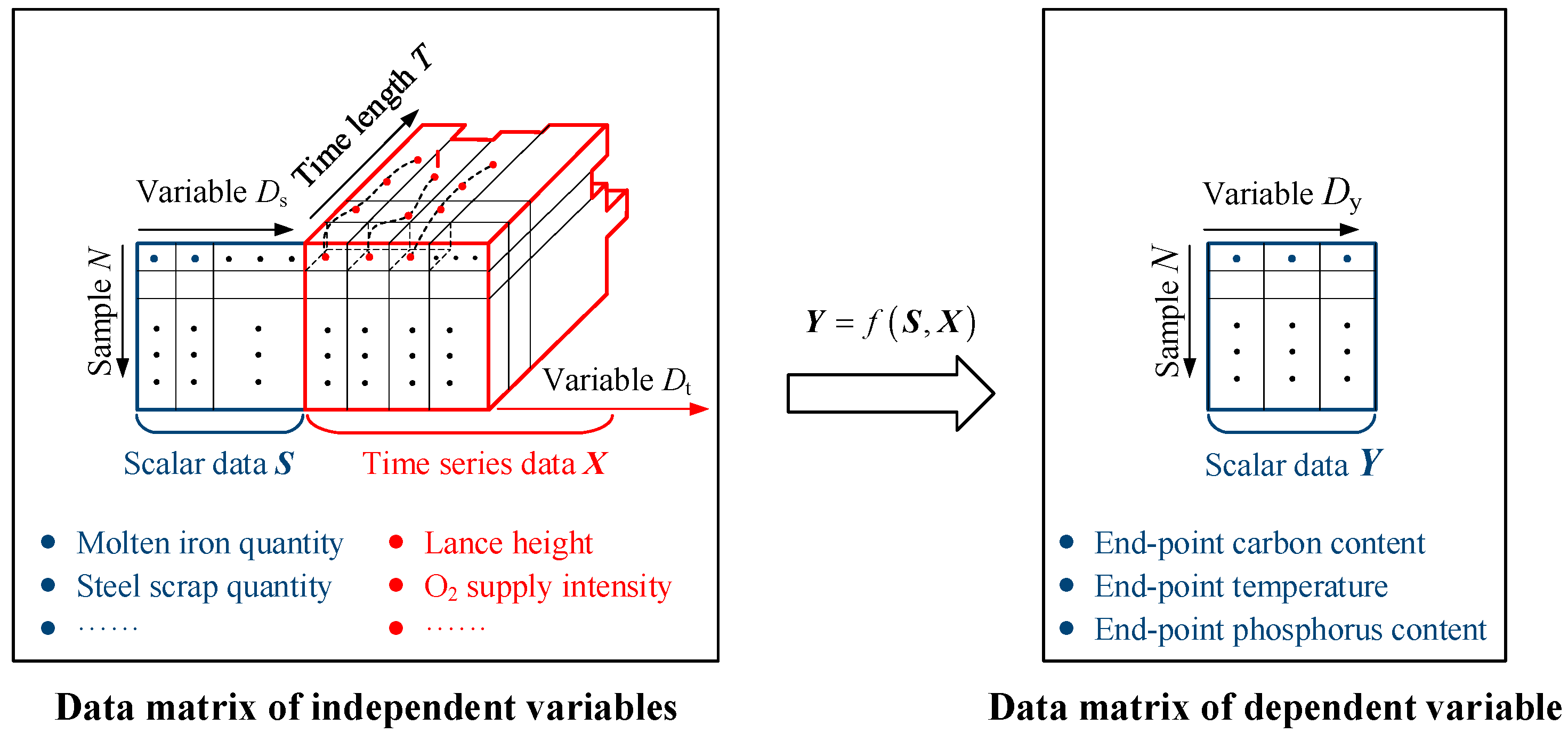
2. Problem Statement

The key task of end-point control of the BOF steelmaking process is to ensure that the final carbon and phosphorous contents and temperature of steel meet the requirements. Accurate control of the end-point can decrease the number of additional blows, which is of great significance for improving production efficiency, reducing production costs, and stabilizing the properties of the final product. However, steelmaking is a process with a long production cycle, complex physical and chemical reactions, large fluctuations in raw materials, strong time variability in the blowing process, unstable process control, and a heavy reliance on manual experience. Traditional prediction models such as MLRP models and NNP models exhibit the following limitations when applied to predicting the final properties of BOF steelmaking.

• The BOF steelmaking process includes both scalar data such as raw material properties and time series data such as the process parameters of the blowing process. Traditional prediction models still have certain limitations in capturing the nonlinear and time-varying characteristics of steelmaking data containing mixed data types, especially time series data.
• The final carbon and phosphorous contents and temperature of steel are not only affected by a variety of input variables but also the complex non-linear coupling relationships between these property indicators. For example, the temperature will affect the decarburization rate and dephosphorization rate, which will in turn affect the carbon content and phosphorus content. At different blowing stages, changes in carbon content will have different effects on the dephosphorization rate. Traditional prediction models ignore the mutual coupling relationships between property indicators, and it is necessary to further improve the accuracy of the simultaneous prediction of multiple property indicators.

In order to solve the above problems, deep learning technology is used to establish a multi-output prediction model for BOF steelmaking. The main idea of the model is shown in Figure 1.

Scalar data such as raw material properties provide key physical and chemical parameters relevant to the steelmaking process. These data have a direct impact on the final carbon content, phosphorus content, and temperature. Time series data such as lance height provide information on dynamic changes occurring during the blowing process. For instance, changes in oxygen supply intensity will affect the decarburization rate and thus the final carbon content. Hence, both scalar and time series data serve as input variables for the model. Deep network structures can be used to extract features of mixed input variables. The mapping relationship $f$ between output variables and input variables is established to predict multiple output variables by inputting multiple variables. The improved accuracy and reliability of the final prediction will provide data guidance for dynamically controlling the steelmaking process.

3. Methodology

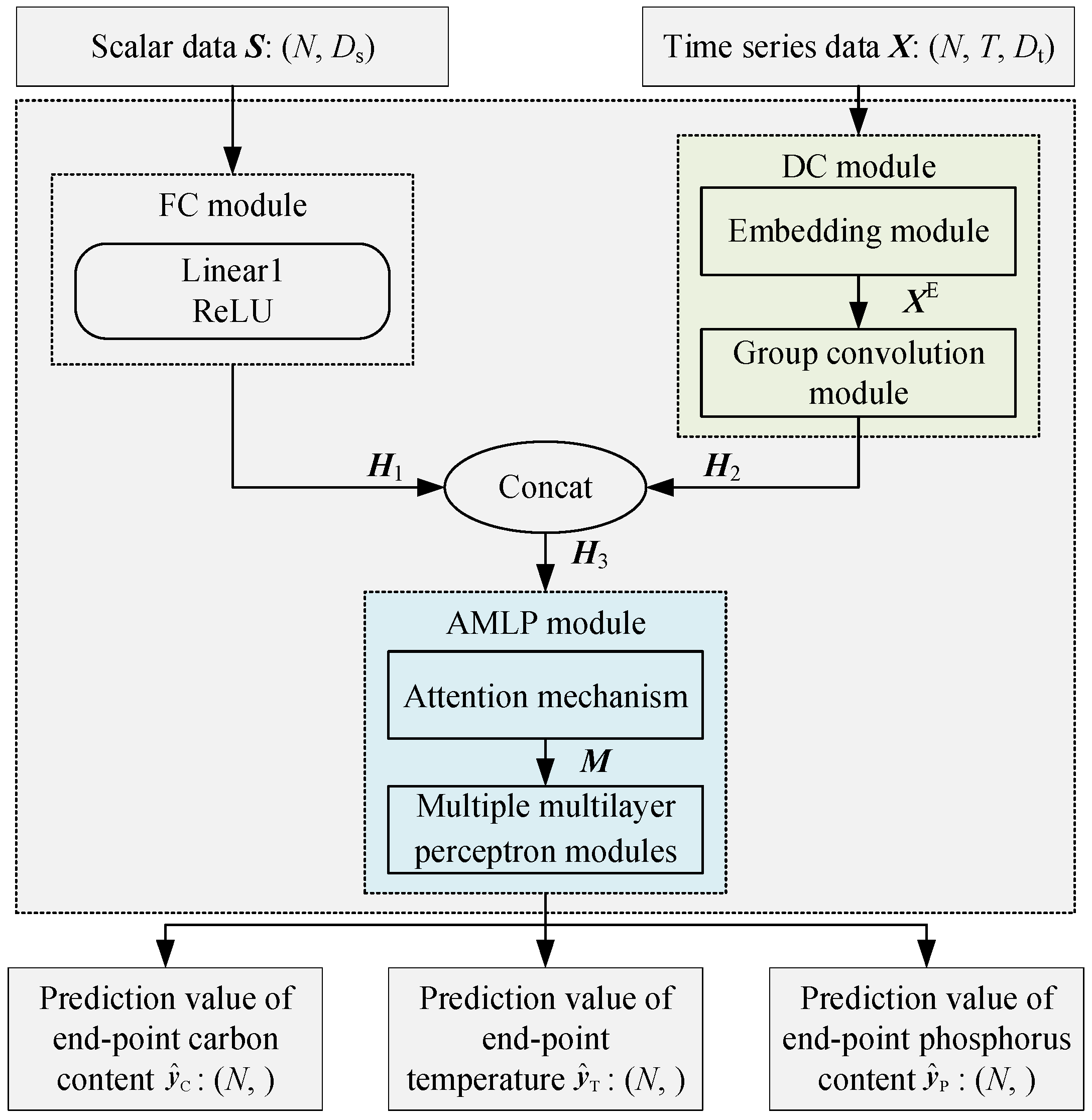
3.1. Network Structure

BOF steelmaking data include scalar data such as properties of raw materials and time series data based on process parameters. Let ${\mathit{A}}_{\mathrm{tr}}={\left\{\left(\mathit{S},\mathit{X}\right)\right\}}_{n=1}^N$ represent the training dataset. Let $\mathit{S}=\left\{s_{n1},s_{n2},\cdots ,s_{n{D}_s}\right\}$, $n=1,2,\dots ,N$, $\mathit{S}\in {\Re }^{N\times D_s}$ be a vector space of scalar variables, where $n$ represents the number of samples and $D_{\mathrm{s}}$ is the dimension of scalar variables. Let $\mathit{X}=\left\{{\mathit{x}}_1,\cdots ,{\mathit{x}}_t,\cdots ,{\mathit{x}}_T\right\}$, $\mathit{X}\in {\Re }^{N\times T\times D_{\mathrm{t}}}$ be a vector space of time series variables, where ${\mathit{x}}_t={\left[{\mathit{x}}_{t1},{\mathit{x}}_{t2},\cdots ,{\mathit{x}}_{t{D}_{\mathrm{t}}}\right]}^{\mathrm{T}}$ represents the observed values of all variables at the $t$-th moment, $T$ represents the time length of time series variables, and $D_{\mathrm{t}}$ represents the dimension of the time series variables.

The network architecture of the FDCAN model, shown in Figure 2, primarily comprises a fully connected (FC) module, a deep convolution (DC) module, and an attention-augmented multi-layer perceptron (AMLP) module. The FC module is utilized for extracting features from scalar data. The DC module is employed to capture the characteristics inherent in time series data. The AMLP module serves the dual purpose of learning feature representations from heterogeneous data and predicting multiple output variables.

The FC module is employed to extract nonlinear features within scalar data and consists of a linear layer followed by a ReLU activation function, as shown in the left branch in Figure 2. The output ${\mathit{H}}_1$ of the FC module can be represented as follows:

$${\mathit{H}}_1=\mathrm{ReLU}\left({\mathit{W}}_1\mathit{S}+{\mathit{b}}_1\right)$$

(1)

where ${\mathit{W}}_1$ and ${\mathit{b}}_1$ represent the weight and bias of Linear1, while $\mathrm{ReLU}\left(\right)$ denotes the activation function.

The network structures of the DC module and AMLP module are introduced in detail in Section 3.2 and Section 3.3.

3.2. Deep Convolution Module

The DC module consists of two parts: the embedding (Embed) module and the group convolution (GC) module. Specifically, the embedding module maps the original data to a multi-channel dimension space by embedding a channel dimension into the original multivariate time series, which is beneficial to capturing the long dependence of the data in the time dimension. In addition, the group convolution module extracts the characteristics of time series data in the variable dimension and channel dimension through variable group convolution and channel group convolution with different numbers of groups. In summary, the main function of the DC module is to extract feature representations of various dimensions from time series data.

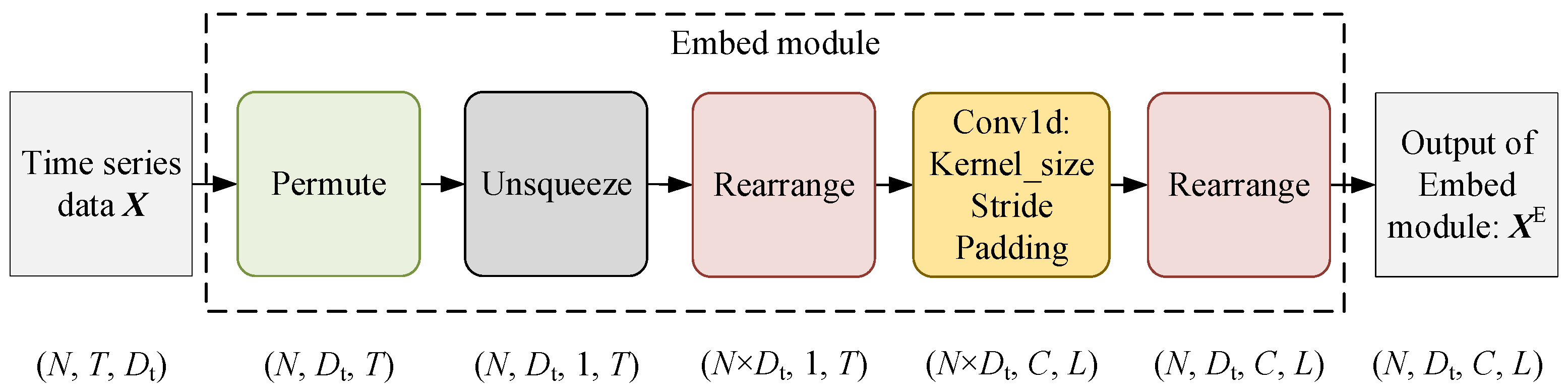
3.2.1. Embedding Module

The original multivariate time series includes a sample dimension, a time dimension, and a variable dimension. The embedding module first embeds a channel dimension based on the three dimensions of the original multivariate time series, with the purpose of mapping the original data into a multi-channel dimensional space to obtain richer information representation. Then, the time series is sliced through the larger convolutional receptive field in one-dimensional convolution (Conv1d) to capture long dependent relationships in the time dimension. The network structure of the embedding module is shown in Figure 3.

The permute function is employed to exchange the time dimension $T$ and variable dimension $D_{\mathrm{t}}$ of the original multivariate time series, resulting in a data shape of $\left(N,D_{\mathrm{t}},T\right)$. Then, the unsqueeze function is applied to add a dimension to the tensor, resulting in a data shape of $\left(N,D_{\mathrm{t}},1,T\right)$. The rearrange function is utilized to merge the dimensions of tensors, resulting in a data shape of $\left(N\times D_{\mathrm{t}},1,T\right)$. One-dimensional convolution is employed to extract features along the time dimension from the data obtained above. Assuming that the number of output channels of one-dimensional convolution is $C$, this results in a data shape of $\left(N\times D_{\mathrm{t}},C,L\right)$. The time length $L$ after the convolution operation can be expressed as the following equation:

$$L=⌊\frac{T-\mathrm{kernel}\_\mathrm{size}+\mathrm{padding}\_\mathrm{left}+\mathrm{padding}\_\mathrm{right}}{\mathrm{stride}}⌋+1$$

(2)

where $\lfloor \rfloor$ represents rounding down, $\mathrm{kernel}\_\mathrm{size}$ represents the convolution kernel size, $\mathrm{padding}\_\mathrm{left}$ and $\mathrm{padding}\_\mathrm{right}$ represent the left and right padding length of the time series, and $\mathrm{stride}$ represents the stride size.

In order to facilitate subsequent data processing, the rearrange function is used to transform the dimensions of the data. Therefore, the data shape of the output feature ${\mathit{X}}^{\mathrm{E}}$ is $\left(N,D_{\mathrm{t}},C,L\right)$ after the original data is processed by the embedding module.

While the number of variables in the original multivariate time series remains unchanged, the embedding module can enhance the richness of the data by increasing the channel dimension, which is beneficial to subsequent feature extraction operations. In addition, the introduction of channel dimensions can characterize the evolution trend of each variable at different time points from different channel dimensions, which is beneficial to capturing complex nonlinear characteristics within the data. At the same time, employing larger convolution kernels in one-dimensional convolution enables the network to acquire a broader receptive field, which helps the network capture longer distance dependencies, thereby improving the performance of the model.

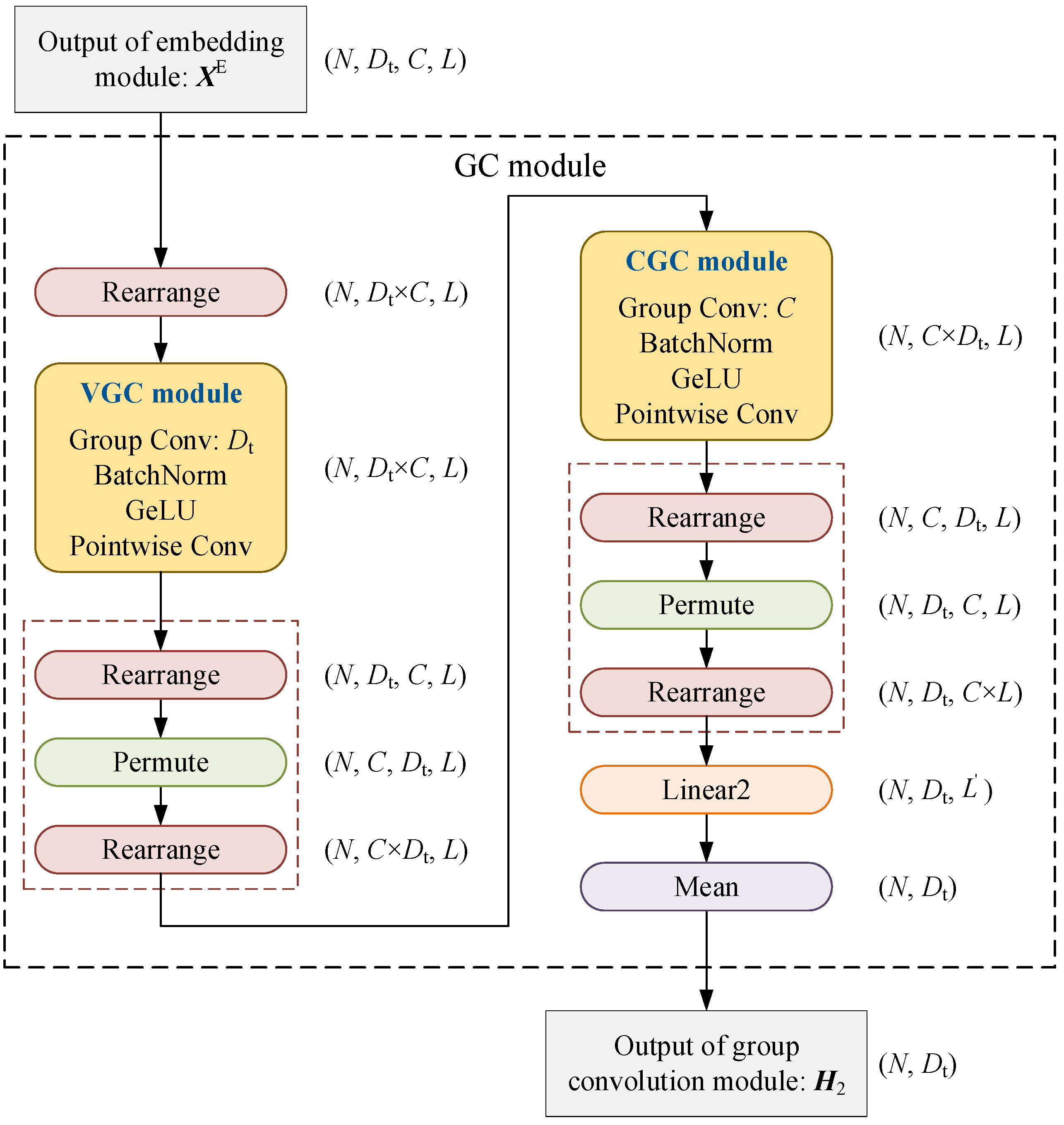
3.2.2. Group Convolution Module

In order to extract the characteristics of multivariate time series in the variable dimension and channel dimension, the group convolution module [34] consists of a variable group convolution (VGC) module, a channel group convolution (CGC) module, and functions such as dimension permute and dimension rearrange. The network structure of the group convolution module is shown in Figure 4.

The rearrange function is employed to multiply the channel dimension and variable dimension of ${\mathit{X}}^{\mathrm{E}}$ output by the embedding module, resulting in a data shape of $\left(N,D_{\mathrm{t}}\times M,L\right)$. The purpose of the above shape transformation is to provide data support for the subsequent extraction of the evolutionary trends of the time series in both the channel and variable dimensions.

The variable group convolution module is composed of a one-dimensional group convolution, a batch normalization, a GeLU activation function, and a pointwise convolution. The number of groups of one-dimensional group convolution in the variable group convolution module is $D_{\mathrm{t}}$, that is, the data are divided into groups $D_{\mathrm{t}}$, with each group containing the time series data for all channels of a variable. Therefore, one-dimensional group convolution can extract the local features of the time series of each variable on all channels.

A batch normalization function and a GeLU activation function are added after the one-dimensional group convolution. Batch normalization introduces noise to the data by randomly sampling the mean and variance of the data. The purpose is to prevent drastic changes in data distribution from causing a decrease in convergence speed. Therefore, batch normalization can reduce the problem of gradient explosion or gradient disappearance during the training process and speed up the convergence of the network. GeLU (Gaussian Error Linear Unit) is an activation function based on the Gaussian error function. Compared with other activation functions such as ReLU, GeLU has a smoother output, which helps improve the convergence speed of the training process. Using one-dimensional group convolution, it is difficult to fuse information between different variables because variables are used one by one. Consequently, a pointwise convolution is introduced following one-dimensional group convolution, batch normalization, and the GeLU activation function. The output channels of pointwise convolution are equal to the input channels because the convolution kernel size is 1. Pointwise convolution can achieve linear transformation between variables without changing the time dimension of the input features. Thus, pointwise convolution can obtain new feature representations that incorporate information between various variables. In summary, the variable group convolution module is capable of simultaneously capturing time series information within and across variables. The equation of the variable group convolution module is as follows:

$${\mathit{X}}^{\mathrm{out}}=\mathrm{PWconv}\left(\mathrm{B}\left(\mathrm{GeLU}\left(\mathrm{Gconv}\left({\mathit{X}}^{\mathrm{in}}\right)\right)\right)\right)$$

(3)

where ${\mathit{X}}^{\mathrm{in}}$ and ${\mathit{X}}^{\mathrm{out}}$ denote the input and output of the variable group convolution module, respectively. $\mathrm{Gconv}\left(\right)$ represents a one-dimensional group convolution. $\mathrm{GeLU}\left(\right)$ represents the GeLU activation function. $\mathrm{B}\left(\right)$ represents batch normalization. $\mathrm{PWconv}\left(\right)$ represents pointwise convolution.

The channel group convolution module has the same network structure as the variable group convolution module and is composed of one-dimensional group convolution, batch normalization, the GeLU activation function, and point-wise convolution. The number of groups of one-dimensional group convolution in the channel group convolution module is $C$, that is, the data are divided into $C$ groups, with each group containing the time series data of all variables of one channel. Therefore, one-dimensional group convolution can extract the local features of the time series of each channel on all variables. The channel group convolution module can simultaneously capture the time series information of all variables within and between channels of time series data.

The group convolution module uses variable group convolution and channel group convolution with different numbers of groups to extract features in the channel dimension and variable dimension of time series data. It is worth mentioning that operations such as rearrange and permute are performed between the two group convolutions in order to correctly group the time series data in the variable dimension and channel dimension. After the utilization of the variable group convolution module and the channel group convolution module to fully extract the time-varying features of the time series data, Linear2 is used to map the time dimension features to a lower dimension, that is, the shorter time dimension $L\prime$. Finally, the Mean function is applied to compress the time dimension to retain the variable dimension of the extracted features, resulting in a data shape of ($N,D_{\mathrm{t}}$). The features of the scalar and time series data extracted by the fully connected module and the group convolution module are input to the attention-augmented multi-layer perceptron module.

3.3. Attention-Augmented Multi-Layer Perceptron Module

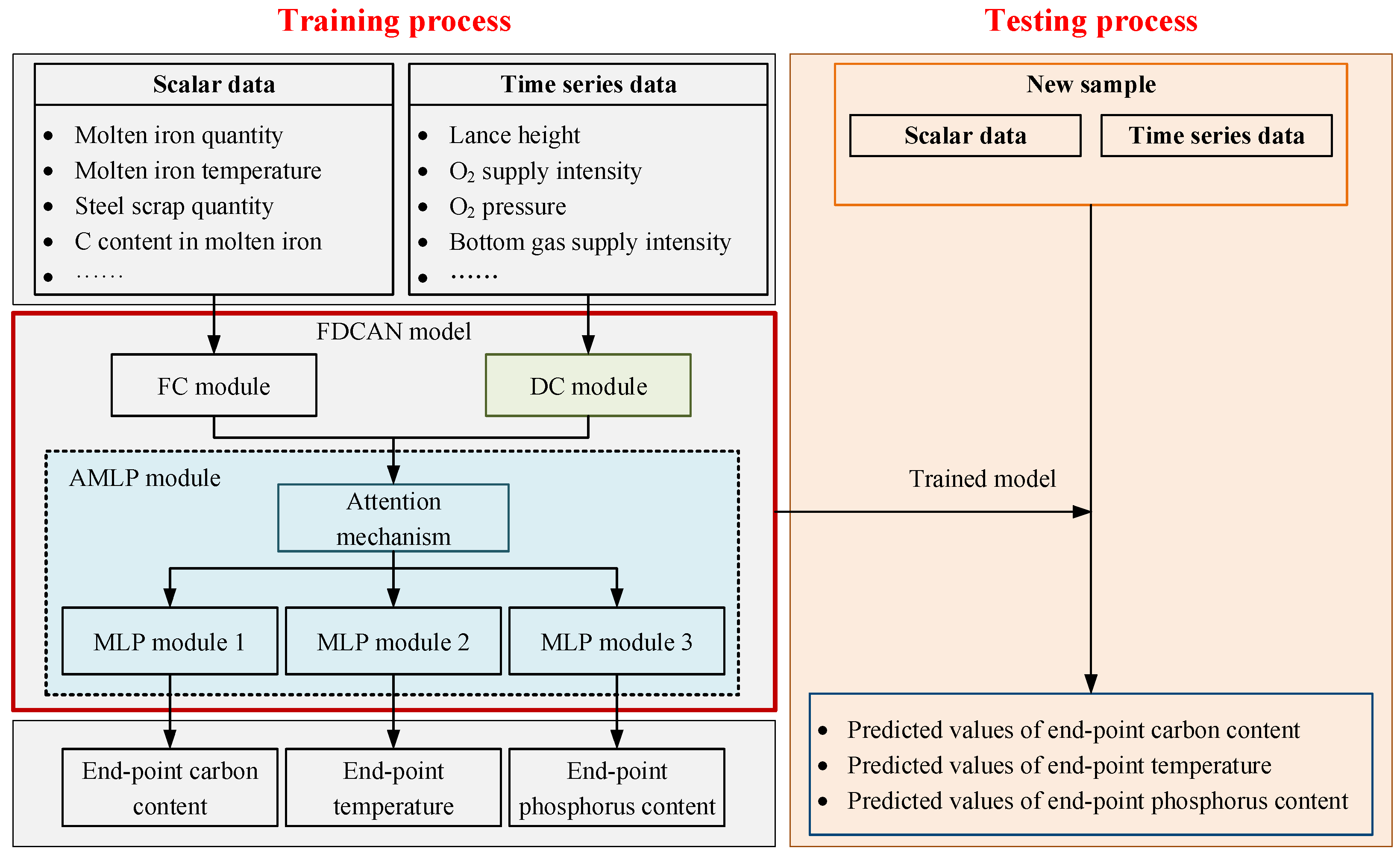
The attention-augmented multi-layer perceptron module consists of an attention mechanism and multiple multilayer perceptron (MLP) modules. The network structure of the attention-augmented multi-layer perceptron module is shown in Figure 5.

The attention mechanism is employed to jointly extract features of scalar and time series data. Feature ${\mathit{H}}_1$ of scalar data extracted by the FC module and feature ${\mathit{H}}_2$ of time series data extracted by the DC module are concatenated along the variable dimension to obtain the mixed feature ${\mathit{H}}_3$:

$${\mathit{H}}_3=\mathrm{cat}\left({\mathit{H}}_1,{\mathit{H}}_2\right)$$

(4)

where $\mathrm{cat}\left(\right)$ represents the concatenate.

In order to facilitate focusing on features relevant to the prediction task, the mixed feature ${\mathit{H}}_3$ is input into the attention mechanism, which consists of a linear layer and the ReLU activation function. The mixed features are mapped to a new representation space through linear transformation, and the ReLU activation function is used to increase the nonlinear expression ability of the model. Hence, the attention mechanism can be employed to obtain the corresponding weights of different features. The calculation equation of attention weight $\mathit{S}$ is as follows:

$$\mathit{S}=\mathrm{ReLU}\left({\mathit{W}}_3{\mathit{H}}_3+{\mathit{b}}_3\right)$$

(5)

where ${\mathit{W}}_3$ and ${\mathit{b}}_3$ represent the weight and bias of Linear3.

Multiply the weight $\mathit{S}$ obtained by the attention mechanism and the corresponding elements of feature ${\mathit{H}}_3$ to obtain feature $\mathit{M}$ with different weights. It is worth noting that Linear3 has the same input dimensions and output dimensions. The advantages of the design are that it not only simplifies the structure of the model but also allows the model to keep the dimensions of the features unchanged during the learning process, making it easier to transfer and combine information. Therefore, the value ${\mathit{m}}^{\left(j\right)}$ of the $j$-th feature of the weighted feature $\mathit{M}$ can be expressed as follows:

$${\mathit{m}}^{\left(j\right)}={\mathit{h}}_3^{\left(j\right)}\odot {\mathit{s}}^{\left(j\right)}$$

(6)

where ${\mathit{s}}^{\left(j\right)}$ represents the $j$-th feature in tensor $\mathit{S}$, ${\mathit{h}}_3^{\left(j\right)}$ represents the $j$-th feature in tensor ${\mathit{H}}_3$, and $\odot$ denotes multiplying the elements at corresponding positions in the two vectors.

The attention mechanism is used to assign different weights to mixed features, which helps the module to pay more attention to the key information in the mixed features. Moreover, the attention mechanism is followed by three multi-layer perceptron modules, which are used to predict the final carbon and phosphorus contents and temperature. Each multi-layer perceptron module is composed of multiple linear layers and non-linear activation functions, which can perform in-depth learning and representation of weighted mixed features and mine complex features that are strongly related to each prediction target. Furthermore, each multi-layer perceptron module is used to independently learn specific features relevant to the respective prediction target, rather than mixing features from all variables. Therefore, the design of the branching structure helps to decouple the characteristic relationships between different dependent variables. The equations of the three multi-layer perceptron modules are as follows:

$$\begin{array}{l}{\widehat{\mathit{y}}}_{\mathrm{C}}=\mathrm{Sigmoid}\left({\mathit{W}}_5\left(\mathrm{ReLU}\left({\mathit{W}}_4\mathit{M}+{\mathit{b}}_4\right)\right)+{\mathit{b}}_5\right)\\ {\widehat{\mathit{y}}}_{\mathrm{P}}=\mathrm{Sigmoid}\left({\mathit{W}}_7\left(\mathrm{ReLU}\left({\mathit{W}}_6\mathit{M}+{\mathit{b}}_6\right)\right)+{\mathit{b}}_7\right)\\ {\widehat{\mathit{y}}}_{\mathrm{T}}=\mathrm{Sigmoid}\left({\mathit{W}}_9\left(\mathrm{ReLU}\left({\mathit{W}}_8\mathit{M}+{\mathit{b}}_8\right)\right)+{\mathit{b}}_9\right)\end{array}$$

(7)

where ${\widehat{\mathit{y}}}_{\mathrm{C}}$, ${\widehat{\mathit{y}}}_{\mathrm{T}}$, and ${\widehat{\mathit{y}}}_{\mathrm{P}}$ represent the predicted values of end-point carbon content, temperature, and phosphorus content, ${\mathit{W}}_4$ and ${\mathit{b}}_4$, ${\mathit{W}}_5$ and ${\mathit{b}}_5$, ${\mathit{W}}_6$ and ${\mathit{b}}_6$, ${\mathit{W}}_7$ and ${\mathit{b}}_7$, ${\mathit{W}}_8$ and ${\mathit{b}}_8$, and ${\mathit{W}}_9$ and ${\mathit{b}}_9$ represent the weight and bias of Linear4, Linear5, Linear6, Linear7, Linear8, and Linear9.

The objective of the FDCAN model is to precisely predict the end-point carbon content, temperature, and phosphorus content simultaneously. The FDCAN model uses the mean squared error (MSE) loss function, which is as follows:

$$L=\frac{1}{N}{\displaystyle \sum _{i=1}^N{\left({\mathit{y}}_i-{\widehat{\mathit{y}}}_i\right)}^2}$$

(8)

where $N$ is the number of samples, ${\mathit{y}}_i$ is the true value of end-point carbon content, temperature, and phosphorus content, and ${\widehat{\mathit{y}}}_i$ is the predicted value of end-point carbon content, temperature, and phosphorus content.

3.4. Flow of FDCAN

The training and testing process of the proposed FDCAN model is shown in Figure 6. The training process is as follows.

• Normalize the training set sample ${\mathit{A}}_{\mathrm{tr}}$ to eliminate the influence of dimension.
• Initialize the global parameters of the FDCAN model, including the maximum number of iteration epochs, the sample batch size, the learning rate lr, and the weight decay wd.
• Use the fully connected module to extract features of scalar data and obtain hidden features ${\mathit{H}}_1$;
• Use the embedding module and deep convolution module to extract the characteristics of time series data in the time dimension, variable dimension, and channel dimension to obtain hidden features ${\mathit{H}}_2$;
• Hidden features ${\mathit{H}}_1$ and ${\mathit{H}}_2$ are concatenated to obtain ${\mathit{H}}_3$, which is input into the attention mechanism of the attention-augmented multi-layer perceptron module to obtain hidden features $\mathit{M}$. Multiple multi-layer perceptron modules are used to predict multiple output variables.
• Employ the MSE loss to measure the difference between the predicted and real values. The Adam optimizer is applied to update the FDCAN model.
• Train the FDCAN model and obtain the prediction results of the training set.

The testing process of the FDCAN model is as follows.

• The maximum and minimum values of each variable in the training dataset are used to normalize the testing dataset.
• The trained FDCAN model is employed to obtain the predicted values of final carbon content, temperature, and phosphorus content of new samples in the testing dataset.

4. Experiment on BOF Steelmaking

4.1. Data Description

The data on BOF steelmaking are collected from a 260-ton converter in the steelmaking department of a steel plant. The steel types involved in the data are low-carbon medium-phosphorus steels, which adopt a low-carbon pulling process and a single slag process. The low-carbon pulling process involves reducing the carbon content in steel by optimizing the blowing process, adding appropriate cooling agents, and fine-tuning the end-of-blow operations to achieve the desired low carbon levels, thereby improving the properties of the steel. The target end-point carbon content is 0.04 wt%. The upper limit of the target end-point phosphorus content is 0.035 wt%. The target tapping temperature for each heat is provided by the process card. The original data need to be preprocessed, including eliminating missing values and outliers. A total of 724 heats of data are obtained. In order to accurately predict the final carbon content, temperature, and phosphorus content, it is necessary to select independent variables that are highly correlated with the dependent variables according to the metallurgical mechanism [35]. Moreover, these independent variables are able to characterize the physical and chemical reactions and operating conditions during the steelmaking process.

The independent variables that affect the final carbon content, phosphorus content, and temperature mainly include the following variables: (1) Variables related to molten iron include steel scrap quantity, molten iron quantity, molten iron temperature, molten iron carbon, silicon, manganese, phosphorus, and sulfur content. The physical heat of molten iron is the main source of heat balance income for the entire steelmaking process. The addition of scrap steel will absorb heat and lower the temperature. The carbon and phosphorus content of molten iron determine the initial chemical composition of steelmaking. Therefore, these variables have a direct impact on the final carbon content, phosphorus content, and temperature. (2) Oxygen-supply-related variables include lance height, oxygen supply intensity, and oxygen pressure. The control of these variables will affect the distribution and utilization efficiency of heat in the furnace, which in turn affects the control of the carbon oxidation rate, the efficiency of dephosphorization, and the final temperature. (3) Bottom-blow-related variables include bottom air supply intensity. Bottom-blowing gas can enhance the stirring effect of the molten pool and promote the mixing and reaction kinetics inside the molten steel, which is conducive to the decarburization reaction and promotes more efficient dephosphorization. Especially in the last blowing stage, strengthening the bottom air supply intensity can promote the further reaction of carbon and oxygen, help reduce the oxygen content in the molten steel, and thus affect the final temperature. (4) Temperature-related variables are molten iron temperature, TSC (Temperature sampling carbon) temperature, and target tapping temperature. Higher temperatures enhance the oxidation reactions that remove carbon and improve the reaction kinetics, making carbon removal more efficient. Similarly, optimal temperatures facilitate the dephosphorization process by accelerating phosphorus removal reactions and promoting proper slag formation. However, excessively high temperatures can decrease the solubility of phosphorus in slag, leading to its reversion into the steel. Thus, precise temperature control is essential for effectively reducing both carbon and phosphorus content. (5) Variables related to auxiliary materials, including the amount of slagging agent (lime) and coolant (ore). The addition of auxiliary materials absorbs heat, causing a temperature drop in the furnace and affecting the oxidation reaction of carbon. Conversely, the reaction between lime and impurities such as sulfur and phosphorus to form slag is exothermic, potentially increasing the furnace temperature. The FeO content in the slag also influences the decarburization rate. Additionally, the amount of lime affects the slag’s basicity, which in turn influences the phosphorus distribution ratio and removal efficiency. Thus, the careful management of auxiliary materials is essential for optimizing both carbon and phosphorus removal. Additionally, TSC carbon content can directly affect the final carbon content and temperature.

Among the variables mentioned above, variables related to oxygen supply, bottom blowing, and auxiliary materials are sequential process parameters. The entire time series is used for modeling to capture the dynamic changes in the smelting process. Therefore, the above independent variables can comprehensively consider various factors such as material balance, heat balance, chemical composition, and process control in the steelmaking process, thereby more accurately predicting the final carbon content, temperature, and phosphorus content.

According to the above metallurgical mechanism, each sample has 17 independent variables and three dependent variables. The independent variables include 11 scalar variables and six time series variables, and the dependent variables are all scalar variables, as shown in

Table 1. BOF steelmaking process parameters.

Symbols	Data Type	Variable Name	Sampling Frequency/Hz	Min	Max	Mean
v1	Scalar	Steel scrap quantity/t	/	24.48	64.94	44.41
v2		Molten iron quantity/t	/	213.77	269.11	242.58
v3		Molten iron temperature/°C	/	1232	1407	1327.28
v4		C content in molten iron/wt%	/	3.9	4.82	4.48
v5		Si content in molten iron/wt%	/	0.08	0.65	0.35
v6		Mn content in molten iron/wt%	/	0.08	0.20	0.13
v7		P content in molten iron/wt%	/	0.06	0.15	0.10
v8		S content in molten iron/wt%	/	0.001	0.015	0.004
v9		TSC C content/wt%	/	0.07	0.855	0.42
v10		TSC temperature/°C	/	1541	1673	1609.22
v11		Target tapping temperature/°C	/	1620	1705	1675.92
v12	Time series	Lance height/cm	0.5	167	393	/
v13		O2 supply intensity/(m3 · t−1·min−1)	0.5	2.00	4.66	/
v14		O2 pressure/MPa	0.5	1.04	1.50	/
v15		Bottom gas supply intensity/(m3 · t−1·min−1)	0.5	0.002	0.104	/
v16		Amount of slagging agent/kg	0.5	0	20,530	/
v17		Amount of coolant/kg	0.5	0	8430	/
yC	Scalar	TSO C content/wt%	/	0.02	0.07	0.05
yT		TSO temperature/°C	/	1626	1714	1675.09
yP		TSO P content/wt%	/	0.006	0.030	0.016

. The dependent variables are detected by TSO (Temperature sampling oxygen). Slagging agents include light-burned dolomite, activated lime, dolomite, and fluorspar. Coolants include ores and sinter. It is worth mentioning that each heat has a different blowing time. Therefore, the time series data is padded with −1 to the maximum time length of the blowing process. After counting the time length of the process parameters of 724 heats, it is determined that the maximum number of sampling points for the parameters in the blowing process is 605. Therefore, the dimensions of the scalar data and time series data of the independent variable and the scalar data of the dependent variable are 724 × 11, 724 × 605 × 6, and 724 × 3. The data are normalized to the interval (0,1) to eliminate the dimensional influence between process parameters. In addition, the data are denormalized for production applications.

A total of 80% of the 724 samples are randomly selected to construct the training set, and the remaining 20% of samples are used to constitute the testing set. As a result, the training set contains 580 samples. The testing set contains 144 samples.

4.2. Parameter Settings

The Adam optimizer is utilized to optimize parameters in the FDCAN model. Global parameters [36] include the epoch, batchsize, learning rate ($lr$), and weight decay ($wd$). The epoch represents the number of times the model is trained on the training data set. A small epoch may prevent the model from fully learning the data characteristics, thereby affecting the convergence and performance of the model. Conversely, an excessively large epoch may lead the model to overfit and reduce its generalization ability on new data. Typically, the epoch is set within the range of 200 to 400. The batchsize refers to the number of samples included in each batch during the training process. Batch size has a significant impact on gradient update. A reasonable batchsize can help the model converge stably. The batchsize is generally set to a multiple of 32. The learning rate determines the step size at each iteration while updating the parameters of the model based on the gradients of the loss function. It influences the convergence speed and stability of the training process. A learning rate that is too small may slow down convergence, while a learning rate that is too large may cause instability or divergence. Generally, the learning rate is set within the range of 0.001 to 0.01. The weight decay is a regularization technique that adds a penalty term to the loss function proportional to the square of the magnitude of the weights. It helps prevent overfitting by encouraging smaller weights. The weight decay effectively reduces the complexity of the model, improving its generalization ability. Typically, weight decay is set within the range of $1\times {10}^{-6}$ to $1\times {10}^{-4}$. After experimental tuning and verification, the global parameters of the FDCAN model are set as epoch = 300, batchsize = 64, $lr=2\times {10}^{-3}$, and $wd=5\times {10}^{-4}$.

In addition to global parameters, the network structure parameters of the model [37] play a key role in the prediction performance of the model. After experimental verification, the crucial parameter of the FDCAN model is the channel number  of the embedding module. The embedding module is located at the front end of time series data feature extraction. The purpose of embedding channel dimensions is to increase the feature dimension of the data, thereby helping the model capture more complex feature representations. If more channels are embedded, the data will be mapped to a higher dimensional space, and the model will have a larger number of parameters and higher computational complexity. When the number of samples is small, a large number of channels may cause the model to easily overfit. Thus, the number of channels directly affects the performance and generalization ability of the model. Grid search [38] and cross-validation [39] are used to select the optimal number of channels to improve the accuracy of model predictions.

Prediction accuracy can be evaluated by mean relative prediction error (MRPE). MRPE is usually used to measure the relative error between the predicted value and the real value. First, the relative prediction error is calculated separately for each output variable of each sample, and then the mean of the relative prediction errors of all output variables is calculated to obtain the MRPE of the testing dataset. The equation of the MRPE is as follows:

$$\mathrm{MRPE}=\frac{1}{N_{\mathrm{te}}{D}_{\mathit{y}}}{\displaystyle \sum _{i=1}^{N_{\mathrm{te}}}{\displaystyle \sum _{j=1}^{D_y}\frac{\left|y_{ij}-{\widehat{y}}_{ij}\right|}{\left|y_{ij}\right|}\times 100\%}}$$

(9)

where $N_{\mathrm{te}}$ represents the number of testing dataset samples, $D_y$ represents the number of end-point output variables, $y_{ij}$ represents the real value of the $j$-th output variable of the $i$-th sample, and ${\widehat{y}}_{ij}$ represents the predicted value of the $j$-th output variable of the $i$-th sample.

The channel number $C$ is sequentially set to the power of 2 using the grid search method, that is, 1, 2, 4, 8, 16, 32, and 64. The 5-fold cross-validation method is employed to improve the robustness of parameter selection. The mean relative prediction errors of the final carbon content, temperature, and phosphorus content of the testing datasets are shown in Figure 7.

It can be seen from Figure 7 that when the channel number of the embedding module is $C=2$, the final carbon content, temperature, and phosphorus content have the smallest mean relative prediction errors. Therefore, it can be determined that $C=2$ is the optimal number of channels.

The network structure parameter settings of the FC module, Embed module, GC module, and AMLP module of the FDCAN model are shown in

Table 2. Parameter settings of the FDCAN model.

Network	Name	Shape of Input Data	Number of Output Features	Shape of Output Data	Parameters
FC module	Linear1	(64,12)	64	(64,64)	/
Embed module	Conv1d	(64×6,1,605)	2	(64×6,2,151)	kernel_size = 8 stride = 4 padding = (0,4)
GC module	Group Conv1d1	(64,6×2,151)	12	(64,6×2,151)	kernel_size = 1, stride = 1, groups = 6
	Pointwise Conv1d1	(64,6×2,151)	12	(64,6×2,151)	kernel_size = 1, stride = 1
	Group Conv1d2	(64,2×6,151)	12	(64,2×6,151)	kernel_size = 1, stride = 1, groups = 2
	Pointwise Conv1d2	(64,2×6,151)	12	(64,2×6,151)	kernel_size = 1, stride = 1
	Linear2	(64,6,302)	20	(64,6,20)	/
AMLP module	Linear3	(64,70)	70	(64,70)	/
	Linear4	(64,70)	32	(64,32)	/
	Linear5	(64,32)	1	(64,1)	/
	Linear6	(64,70)	32	(64,32)	/
	Linear7	(64,32)	1	(64,1)	/
	Linear8	(64,70)	32	(64,32)	/
	Linear9	(64,32)	1	(64,1)	/

. The parameters of full connection mainly include the number of output features. The parameters of convolution mainly include the number of output channels, the convolution kernel size (kernel_size), the stride size, the padding size, and the number of groups in group convolution.

4.3. Prediction Result

The FDCAN model is trained using the training dataset, and the trained model is used on 144 samples of the testing dataset of the same steel type as the training set. The comparison between the predicted and real values of the final carbon content, temperature, and phosphorus content of the 144 samples in the testing dataset is shown in Figure 8.

As can be seen from Figure 8, the predicted value of the end-point carbon content is closest to the real value compared with the end-point temperature and the end-point phosphorus content. The above results show that the FDCAN model can effectively capture the key features that affect the final carbon content, making the changes in carbon content easier to identify and predict by the model relative to changes in temperature and phosphorus content. Comparing the predicted values and the real values of the final phosphorus content, it can be found that there is a large prediction error in the range of 0.025 wt% to 0.03 wt% regarding the final phosphorus content. This is because there are complex nonlinear correlations between different output variables in the multi-output variable prediction model, which to a certain extent causes interference in the feature representation learned by the model, thereby affecting the prediction accuracy of phosphorus content.

The performance of different prediction models is verified using the same training and testing data from BOF steelmaking. The ANN (Artificial neural network) [27], DCNN (Deep convolutional neural network) [28], SD-DBN (Supervised dual-branch deep belief network) [29], PCA-BP [30], MC-BP (Monotone-constrained BP) [32], and LSTM [33] models are trained for comparison with the FDCAN model. The trained models are used to obtain the predicted values of the end-point parameters for the testing dataset. Among the above six comparison models, except for the SD-DBN model, which can predict the final carbon content and temperature at the same time, the other five models are all multi-input single-output prediction models. The parameters of the six prediction models are tuned using the cross-validation method, so the prediction results are obtained under optimal conditions. The mean relative prediction errors of the final carbon content, temperature, and phosphorus content of the above seven prediction models are listed in

Table 3. Comparison of the MRPE of different models.

No.	Model	${\mathbf{MRPE}}_{\mathbf{C}}$ *	${\mathbf{MRPE}}_{\mathbf{T}}$ *	${\mathbf{MRPE}}_{\mathbf{P}}$ *	Remarks
1	FDCAN	13.99	0.57	15.78	Simultaneous prediction model of final carbon content, temperature, and phosphorus content
2	ANN	18.24	/	/	Carbon content prediction model
3	DCNN	/	0.51	/	Temperature prediction model
4	SD-DBN	17.56	0.58	/	Simultaneous prediction model of final carbon content and temperature
5	PCA-BP	/	/	15.82	Phosphorus content prediction model
6	MC-BP	/	/	16.74	Phosphorus content prediction model
7	LSTM	17.44	/	/	Carbon content prediction model

* The mean relative prediction errors of the final carbon content, temperature, and phosphorus content are denoted as ${\mathrm{MRPE}}_{\mathrm{C}}$, ${\mathrm{MRPE}}_{\mathrm{T}}$, and ${\mathrm{MRPE}}_{\mathrm{P}}$.

.

As can be seen from Table 3, the mean relative prediction error between the predicted value and the real value of the final carbon content is 13.99%. The mean relative prediction error between the predicted value and the real value of the end-point temperature is 0.57%. The mean relative prediction error between the predicted value and the real value of the final phosphorus content is 15.78%. Compared with the other prediction models, the FDCAN model has the smallest MRPE values for final carbon content and phosphorus content. The results show that the FDCAN model can fully extract the coupling relationships between variables, resulting in superior prediction performance for multiple output variables. While other models, such as the ANN model, can also capture the nonlinearity of mixed data through parameter optimization, the FDCAN model demonstrates higher accuracy. In addition to capturing the nonlinear characteristics of mixed data, the FDCAN model can also learn the temporal variability of time series data, which enhances its ability to accurately predict the final properties of steel.

The final hit rate (HR) is a key property indicator in the BOF steelmaking process. The thresholds are a ±0.015 wt% prediction error range for final carbon content, a ±15 °C prediction error range for final temperature, and a ±0.005 wt% prediction error range for final phosphorus content [30,40]. These thresholds are based on industry standards, which indicate that for low-carbon, medium-phosphorus steel grades, such tolerance levels are acceptable to ensure the properties of the final molten steel [25]. When the predicted values of the final carbon content, temperature, and phosphorus content are within the above threshold ranges, the properties of the final molten steel are considered to reach the target requirements. The final hit rate can be evaluated by calculating the ratio of the number of hits to the total number of samples. The end-point hit rate of the $j$-th variable of molten steel is as follows:

$$h_j=\frac{{\displaystyle \sum _{i=1}^{N_{\mathrm{te}}}{A}_{ij}}}{N_{\mathrm{te}}}$$

(10)

where $A_{ij}$ can be written as $A_{ij}=\left\{\begin{array}{c}1,if\left|y_{ij}-{\widehat{y}}_{ij}\right|\le \mathrm{threshold}\\ 0,f\left|y_{ij}-{\widehat{y}}_{ij}\right|>\mathrm{threshold}\end{array}\right.$. When the predicted value of the $j$-th variable of the $i$-th sample is within the threshold range of the real value, it indicates that the end point is hit and is recorded as 1; otherwise, it is recorded as 0.

For the 144 samples in the testing dataset, the prediction results of the six prediction models for the final carbon content within the ±0.015 wt% error range, the final temperature within the ±15 °C error range, and the final phosphorus content within the ±0.005 wt% error range are shown in Figure 9, Figure 10 and Figure 11.

It can be seen from Figure 9, Figure 10 and Figure 11 that compared with other models, the results predicted by the FDCAN model are closer to the real values. The scattered points predicted by the FDCAN model are more concentrated and closely distributed between the center line and the threshold range. In addition, other models can only obtain high prediction accuracy on one or two output variables, and cannot achieve high prediction accuracy on three output variables at the same time. For example, the SD-DBN model has a high hit rate in predicting the final carbon content but a low hit rate in predicting the final temperature. The above results show that the FDCAN model can maintain stable prediction performance when multiple property indicators are coupled with each other. Therefore, the FDCAN model has high robustness and helps provide a reference for final control in the actual production process.

A total of seven prediction models, FDCAN, ANN, DCNN, SD-DBN, PCA-BP, MC-BP, and LSTM, are employed in the BOF steelmaking process. The hit rates for the final carbon content within the error range of ±0.015 wt%, the final temperature within the error range of ±15 °C, and the final phosphorus content within the error range of ±0.005 wt%, as well as the number of parameters of different models and the computation efficiency of the training process and testing process, are listed in

Table 4. Comparison of the performance of different prediction models.

No.	Model	Hit Rate of [C]/%	Hit Rate of [T]/%	Hit Rate of [P]/%	Number of Parameters	Computation Efficiency
						Training/s	Testing/ms
1	FDCAN	95.14	84.72	88.89	19,643	63.525	0.692
2	ANN	89.58	/	/	24,897	127.402	0.894
3	DCNN	/	85.42	/	54,081	455.379	1.850
4	SD-DBN	87.50	81.94	/	32,450	349.968	1.493
5	PCA-BP	/	/	86.81	25,025	66.059	0.751
6	MC-BP	/	/	88.19	30,465	79.163	0.743
7	LSTM	90.97	/	/	28,135	56.303	0.634

.

Compared with the other six models in Table 4, the FDCAN model can predict three end-point properties simultaneously. Specifically, the FDCAN model has the largest number of samples, with final carbon and phosphorus contents falling within the target range. This means that the final carbon content and phosphorus content predicted by the FDCAN model have the highest final hit rates. The above results show that the FDCAN model can accurately predict the final composition of the BOF steelmaking process, satisfying the target requirements for the properties. In terms of the number of parameters and computational efficiency, the FDCAN model stands out, with the fewest parameters and a training time that is second only to the LSTM model. The FDCAN model needs to be trained only once to simultaneously obtain the three final properties of molten steel. Additionally, it achieves higher prediction accuracy for final carbon content compared to the LSTM model. When predicting the final carbon content, phosphorus content, and temperature of molten steel, training the LSTM model three times would consume more computational resources. Other single-variable prediction models, such as the DCNN model, although slightly more accurate in predicting final temperature, require 54,081 parameters and a training time of 455.379 s, which is seven times longer than that of the FDCAN model. Predicting all three final properties with the DCNN model would result in an enormous parameter count and an even longer training time. Therefore, the significant advantage of the FDCAN model lies in its ability to simultaneously predict multiple final properties of molten steel with minimal parameters and high computational efficiency. The FDCAN model consumes fewer memory resources, making it more suitable for deployment in industrial environments. This efficiency aids on-site staff in promptly adjusting process parameters, thereby providing robust support for production decisions.

The experiments are conducted on a personal computer with a Core i7-12700K, 2.10-GHz processor, Nvidia 3090 GPU, and 24 GB RAM. The operating system is a 64-bit version of Linux Ubuntu. The program has been developed using PyCharm, and the programming language is Python. In terms of the computational efficiency of the test process, the final prediction time for the new sample is approximately 0.692 milliseconds. The highest sampling frequency of data in the BOF steelmaking process is 0.5 Hz, that is, the minimum sampling interval is 2 s, which is much longer than the testing process of the FDCAN model. In conclusion, in terms of end-point hit rates and computational efficiency, the proposed FDCAN model can meet the requirements for the accurate prediction of final properties in BOF steelmaking. Moreover, the proposed FDCAN model is sufficient to keep up with the real-time dynamic control of the process, which ensures that the digital twin can effectively support dynamic control in BOF steelmaking.

5. Discussion

The proposed FDCAN model contains an embedding module, a group convolution module, an attention mechanism, and multiple multi-layer perceptron modules in the attention-augmented multi-layer perceptron module.

Table 5. Results of structural ablation experiments of the FDCAN model.

No.	Structural Description	Hit Rate of [C]/%	Hit Rate of [T]/%	Hit Rate of [P]/%
1	FDCAN model	95.14	84.72	88.89
2	Remove the Embed module	70.83	75.69	80.56
3	Remove the GC module	85.42	57.64	81.25
4	Remove the attention mechanism	81.94	75.69	85.42
5	Remove the MLP module	80.56	70.14	75.69

lists five sets of structural ablation experiments to verify the effectiveness of the above structures through the hit rate of final carbon content, temperature, and phosphorus content. It is worth mentioning that a fully connected layer is used to replace the removed modules to complete the shape transformation of the data in the ablation experiment.

As can be seen from Table 5, all structures of the FDCAN model contribute to improving the prediction accuracy of final property indicators. The Embed module can embed a new channel dimension in time series data and map the data to a high-dimensional channel space. In addition, the one-dimensional convolution in the Embed module can learn the relationship between different time points in the data, which is beneficial to obtaining long-term dependencies in time series data. The GC module uses variable group convolution and channel group convolution to extract local features in time series data from the variable dimension and channel dimension, respectively. Convolution has the property of translation invariance, allowing it to combine local features in time series to obtain more comprehensive feature representation without being affected by the time dimension. This property helps to capture complex patterns in time series data and improves the model’s robustness. The attention mechanism in the AMLP module is used to assign greater weight to important features extracted from scalar and time series data, which can reduce the attention paid to redundant information. Moreover, the attention mechanism can also help to selectively focus on key features, which not only improves the efficiency of the model in extracting and utilizing key information in the data but also improves the performance of the model. Multiple MLP modules can integrate multiple related but not identical tasks into one model and share the representation of underlying features, which is beneficial to improving data utilization efficiency and reducing the risk of model overfitting. In addition, different MLP modules have different parameters, which can better adapt to the characteristics of different dependent variables and help improve the generalization ability of the model. In summary, the hierarchical feature learning structure of the FDCAN model can extract features at different levels from the original data and realize feature interaction, integration, and refinement, which helps capture crucial information in the data that is beneficial to the final prediction. Removing any of the above structures will lead to poorer prediction accuracy and lower hit rates. Therefore, the above results prove the effectiveness of each module in the FDCAN model.

6. Conclusions

This paper proposes a multi-output prediction model for the final properties of steel in the BOF steelmaking process based on the fusion of deep convolution and attention mechanism networks (FDCAN). The FDCAN model utilizes an embedding module to map time series data, such as lance height, oxygen supply intensity, and bottom air supply intensity during the blowing process, into a high-dimensional feature space, capturing long-term dependencies. In addition, the deep convolutional network extracts local features of time series data across the channel, variable, and time dimensions, allowing the model to handle complex sequence trends and maintain robustness with mixed input data.

The FDCAN model employs the attention mechanism to assign greater weight to key features with significant importance. Multiple multi-layer perceptron modules share the same underlying feature representation while adapting to the predictive characteristics of different output variables, effectively decoupling complex nonlinear relationships among them. Therefore, the FDCAN model can consider the correlation between input variables (e.g., properties of raw materials and lance height), between input variables and output variables (e.g., bottom air supply intensity and final phosphorus content), and between output variables (i.e., final carbon content, temperature, and phosphorus content), thereby enhancing data guidance for end-point control in actual production.

Ablation experiments demonstrate that the embedding module, group convolution module, and attention-augmented multi-layer perceptron module significantly improve the model’s prediction performance. Compared to other prediction models, the FDCAN model achieves the highest hit rate for simultaneous predictions: 95.14% for final carbon content within ±0.015 wt%, 84.72% for final temperature within ±15 °C, and 88.89% for final phosphorus content within ±0.005 wt%, confirming the method’s effectiveness.

References

1. Qian, Q.; Dong, Q.; Xu, J.; Zhao, W.; Li, M. A metallurgical dynamics-based method for production state characterization and end-point time prediction of basic oxygen furnace steelmaking. Metals 2022, 13, 2. [Google Scholar] [CrossRef]
2. Wang, R.; Mohanty, I.; Srivastava, A.; Roy, T.K.; Gupta, P.; Chattopadhyay, K. Hybrid method for endpoint prediction in a basic oxygen furnace. Metals 2022, 12, 801. [Google Scholar] [CrossRef]
3. Wang, Z.; Liu, Q.; Liu, H.; Wei, S. A review of end-point carbon prediction for BOF steelmaking process. High Temp. Mater. Process. 2020, 39, 653–662. [Google Scholar] [CrossRef]
4. Guo, J.-W.; Zhan, D.-P.; Xu, G.-C.; Yang, N.-H.; Wang, B.; Wang, M.-X.; You, G.-W. An online BOF terminal temperature control model based on big data learning. J. Iron Steel Res. Int. 2023, 30, 875–886. [Google Scholar] [CrossRef]
5. Barui, S.; Mukherjee, S.; Srivastava, A.; Chattopadhyay, K. Understanding dephosphorization in basic oxygen furnaces (BOFs) using data driven modeling techniques. Metals 2019, 9, 955. [Google Scholar] [CrossRef]
6. Qing, X.; Niu, Y. Hourly day-ahead solar irradiance prediction using weather forecasts by LSTM. Energy 2018, 148, 461–468. [Google Scholar] [CrossRef]
7. Chen, Z.; Wang, B.; Gorban, A.N. Multivariate Gaussian and Student-t process regression for multi-output prediction. Neural Comput. Appl. 2020, 32, 3005–3028. [Google Scholar] [CrossRef]
8. Li, H.; Barui, S.; Mukherjee, S.; Chattopadhyay, K. Least squares twin support vector machines to classify end-point phosphorus content in BOF steelmaking. Metals 2022, 12, 268. [Google Scholar] [CrossRef]
9. Phull, J.; Egas, J.; Barui, S.; Mukherjee, S.; Chattopadhyay, K. An application of decision tree-based twin support vector machines to classify dephosphorization in bof steelmaking. Metals 2019, 10, 25. [Google Scholar] [CrossRef]
10. Wang, Z.; Xie, F.; Wang, B.; Liu, Q.; Lu, X.; Hu, L.; Cai, F. The Control and Prediction of End-Point Phosphorus Content during BOF Steelmaking Process. Steel Res. Int. 2014, 85, 599–606. [Google Scholar] [CrossRef]
11. Cai, X.-Y.; Duan, H.-J.; Li, D.-H.; Xu, A.-J.; Zhang, L.-F. Water modeling on fluid flow and mixing phenomena in a BOF steelmaking converter. J. Iron Steel Res. Int. 2024, 31, 595–607. [Google Scholar] [CrossRef]
12. Schlautmann, M.; Kleimt, B.; Khadhraoui, S.; Hack, K.; Monheim, P.; Glaser, B.; Antonic, R.; Adderley, M.; Schrama, F. Dynamic on-line monitoring and end point control of dephosphorisation in the BOF converter. In Proceedings of the 3rd European Steel Technology and Application Days (ESTAD), Vienna, Austria, 26–29 June 2017. [Google Scholar]
13. Feng, K.; Xu, A.; He, D.; Wang, H. An improved CBR model based on mechanistic model similarity for predicting end phosphorus content in dephosphorization converter. Steel Res. Int. 2018, 89, 1800063. [Google Scholar] [CrossRef]
14. Li, G.-H.; Wang, B.; Liu, Q.; Tian, X.-Z.; Zhu, R.; Hu, L.-N.; Cheng, G.-G. A process model for BOF process based on bath mixing degree. Int. J. Miner. Metall. Mater. 2010, 17, 715–722. [Google Scholar] [CrossRef]
15. Zhang, C.-J.; Zhang, Y.-C.; Han, Y. Industrial cyber-physical system driven intelligent prediction model for converter end carbon content in steelmaking plants. J. Ind. Inf. Integr. 2022, 28, 100356. [Google Scholar] [CrossRef]
16. Zhang, R.; Yang, J. State of the art in applications of machine learning in steelmaking process modeling. Int. J. Miner. Metall. Mater. 2023, 30, 2055–2075. [Google Scholar] [CrossRef]
17. Gao, C.; Shen, M.; Liu, X.; Wang, L.; Chen, M. End-point prediction of BOF steelmaking based on KNNWTSVR and LWOA. Trans. Indian Inst. Met. 2019, 72, 257–270. [Google Scholar] [CrossRef]
18. Liu, L.; Li, P.; Chu, M.; Gao, C. End-point prediction of 260 tons basic oxygen furnace (BOF) steelmaking based on WNPSVR and WOA. J. Intell. Fuzzy Syst. 2021, 41, 2923–2937. [Google Scholar] [CrossRef]
19. Xin, Z.; Zhang, J.; Jin, Y.; Zheng, J.; Liu, Q. Predicting the alloying element yield in a ladle furnace using principal component analysis and deep neural network. Int. J. Miner. Metall. Mater. 2023, 30, 335–344. [Google Scholar] [CrossRef]
20. Qi, L.; Liu, H.; Xiong, Q.; Chen, Z. Just-in-time-learning based prediction model of BOF endpoint carbon content and temperature via vMF mixture model and weighted extreme learning machine. Comput. Chem. Eng. 2021, 154, 107488. [Google Scholar] [CrossRef]
21. Han, M.; Cao, Z. An improved case-based reasoning method and its application in endpoint prediction of basic oxygen furnace. Neurocomputing 2015, 149, 1245–1252. [Google Scholar] [CrossRef]
22. Gao, C.; Shen, M.; Liu, X.; Zhao, N.; Chu, M. End-point dynamic control of basic oxygen furnace steelmaking based on improved unconstrained twin support vector regression. J. Iron Steel Res. Int. 2020, 27, 42–54. [Google Scholar] [CrossRef]
23. Zhang, R.; Yang, J.; Wu, S.; Sun, H.; Yang, W. Comparison of the Prediction of BOF End-Point Phosphorus Content Among Machine Learning Models and Metallurgical Mechanism Model. Steel Res. Int. 2023, 94, 2200682. [Google Scholar] [CrossRef]
24. Qian, Q.; Li, M.; Xu, J. Dynamic prediction of multivariate functional data based on functional kernel partial least squares. J. Process Control 2022, 116, 273–285. [Google Scholar] [CrossRef]
25. Qian, Q.; Chang, F.; Dong, Q.; Li, M.; Xu, J. Dynamic Prediction with Statistical Uncertainty Evaluation of Phosphorus Content Based on Functional Relevance Vector Machine. Steel Res. Int. 2024, 95, 2300351. [Google Scholar] [CrossRef]
26. Huang, C.; Dai, Z.; Sun, Y.; Wang, Z.; Liu, W.; Yang, S.; Li, J. Recognition of Converter Steelmaking State Based on Convolutional Recurrent Neural Networks. Metall. Mater. Trans. B 2024, 55, 1856–1868. [Google Scholar] [CrossRef]
27. Yang, L.; Li, B.; Guo, Y.; Wang, S.; Xue, B.; Hu, S. Influence factor analysis and prediction model of end-point carbon content based on artificial neural network in electric arc furnace steelmaking process. Coatings 2022, 12, 1508. [Google Scholar] [CrossRef]
28. Song, G.W.; Tama, B.A.; Park, J.; Hwang, J.Y.; Bang, J.; Park, S.J.; Lee, S. Temperature control optimization in a steel-making continuous casting process using a multimodal deep learning approach. Steel Res. Int. 2019, 90, 1900321. [Google Scholar] [CrossRef]
29. Lu, Z.; Liu, H.; Chen, F.; Li, H.; Xue, X. BOF steelmaking endpoint carbon content and temperature soft sensor based on supervised dual-branch DBN. Meas. Sci. Technol. 2023, 35, 035119. [Google Scholar] [CrossRef]
30. He, F.; Zhang, L. Prediction model of end-point phosphorus content in BOF steelmaking process based on PCA and BP neural network. J. Process Control 2018, 66, 51–58. [Google Scholar] [CrossRef]
31. Liu, Z.; Cheng, S.; Liu, P. Prediction model of BOF end-point temperature and carbon content based on PCA-GA-BP neural network. Metall. Res. Technol. 2022, 119, 605. [Google Scholar] [CrossRef]
32. Zhou, K.-X.; Lin, W.-H.; Sun, J.-K.; Zhang, J.-S.; Zhang, D.-Z.; Feng, X.-M.; Liu, Q. Prediction model of end-point phosphorus content for BOF based on monotone-constrained BP neural network. J. Iron Steel Res. Int. 2022, 29, 751–760. [Google Scholar] [CrossRef]
33. Gu, M.; Xu, A.; Wang, H.; Wang, Z. Real-time dynamic carbon content prediction model for second blowing stage in BOF based on CBR and LSTM. Processes 2021, 9, 1987. [Google Scholar] [CrossRef]
34. Wang, X.; Kan, M.; Shan, S.; Chen, X. Fully learnable group convolution for acceleration of deep neural networks. In Proceedings of the IEEE/CVF Conference on Computer Vision and Pattern Recognition, Long Beach, CA, USA, 16–17 June 2019. [Google Scholar]
35. Xie, T.-Y.; Zhang, C.-D.; Zhou, Q.-L.; Tian, Z.-Q.; Liu, S.; Guo, H.-J. TSC prediction and dynamic control of BOF steelmaking with state-of-the-art machine learning and deep learning methods. J. Iron Steel Res. Int. 2024, 31, 174–194. [Google Scholar] [CrossRef]
36. Niu, T.; Wang, J.; Lu, H.; Yang, W.; Du, P. Developing a deep learning framework with two-stage feature selection for multivariate financial time series forecasting. Expert Syst. Appl. 2020, 148, 113237. [Google Scholar] [CrossRef]
37. Triwiyanto, T.; Pawana, I.P.A.; Purnomo, M.H. An improved performance of deep learning based on convolution neural network to classify the hand motion by evaluating hyper parameter. IEEE Trans. Neural Syst. Rehabil. Eng. 2020, 28, 1678–1688. [Google Scholar] [CrossRef] [PubMed]
38. Yao, L.; Fang, Z.; Xiao, Y.; Hou, J.; Fu, Z. An intelligent fault diagnosis method for lithium battery systems based on grid search support vector machine. Energy 2021, 214, 118866. [Google Scholar] [CrossRef]
39. Liland, K.H.; Skogholt, J.; Indahl, U.G. A new formula for faster computation of the k-fold cross-validation and good regularisation parameter values in Ridge Regression. IEEE Access 2024, 12, 17349–17368. [Google Scholar] [CrossRef]
40. Shi, C.; Guo, S.; Wang, B.; Ma, Z.; Wu, C.L.; Sun, P. Prediction model of BOF end-point phosphorus content and sulfur content based on LWOA-TSVR. Ironmak. Steelmak. 2023, 50, 857–866. [Google Scholar] [CrossRef]
Figure 1. The main idea of a multi-output prediction model.
Metals 14 00773 g001
Figure 2. Network architecture of the FDCAN model.
Metals 14 00773 g002
Figure 3. Network structure of the Embed module.
Metals 14 00773 g003
Figure 4. Network structure of the GC module.
Metals 14 00773 g004
Figure 5. Network structure of the AMLP module.
Metals 14 00773 g005
Figure 6. Flowchart of the FDCAN model.
Metals 14 00773 g006
Figure 7. Channel number selection for the embedding module.
Metals 14 00773 g007
Figure 8. Comparison of predicted and real values. (a) End-point carbon content, (b) End-point temperature, and (c) End-point phosphorus content.
Metals 14 00773 g008
Figure 9. Comparison of hit rates for end-point carbon content. (a) FDCAN model, (b) ANN model, (c) SD-DBN model, and (d) LSTM model.
Metals 14 00773 g009
Figure 10. Comparison of hit rates for end-point temperature. (a) FDCAN model, (b) DCNN model, and (c) SD-DBN model.
Metals 14 00773 g010
Figure 11. Comparison of hit rates for end-point phosphorus content. (a) FDCAN model, (b) PCA-BP model, and (c) MC-BP model.
Metals 14 00773 g011