Energy and Structure of the Terbium Domain Wall


Abstract
:1. Introduction
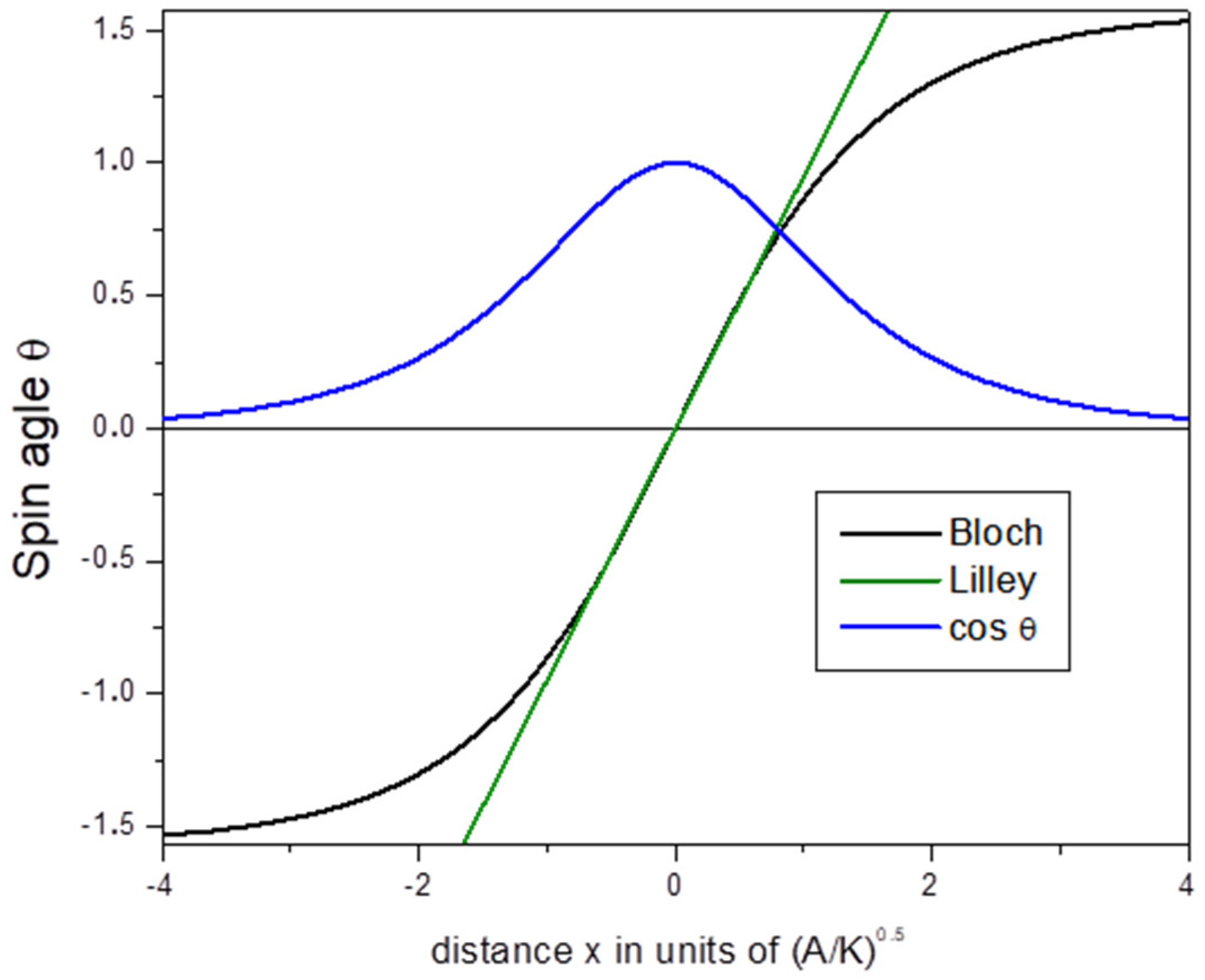
2. The Bloch Model
3. The Egami Model
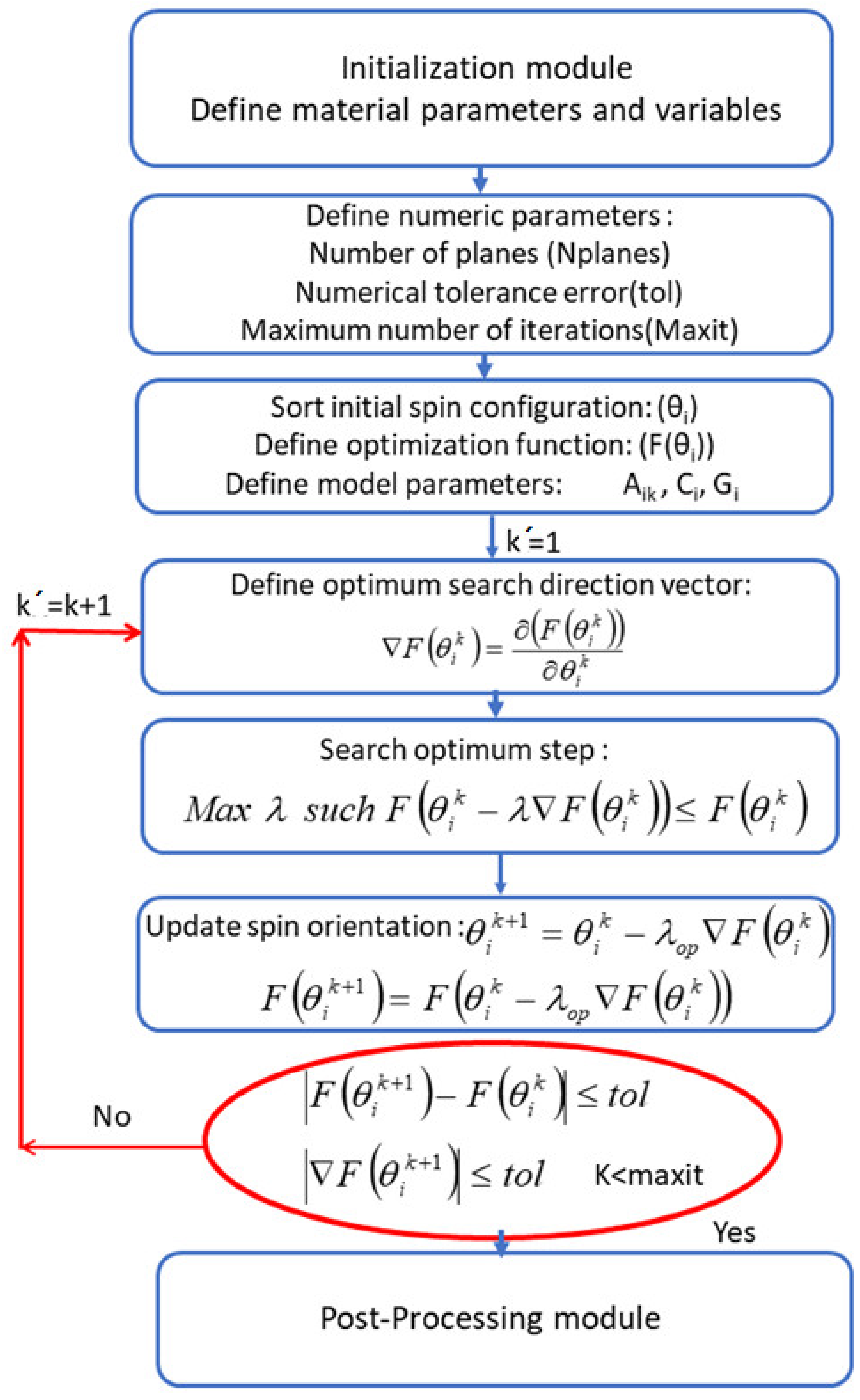
Model Solution
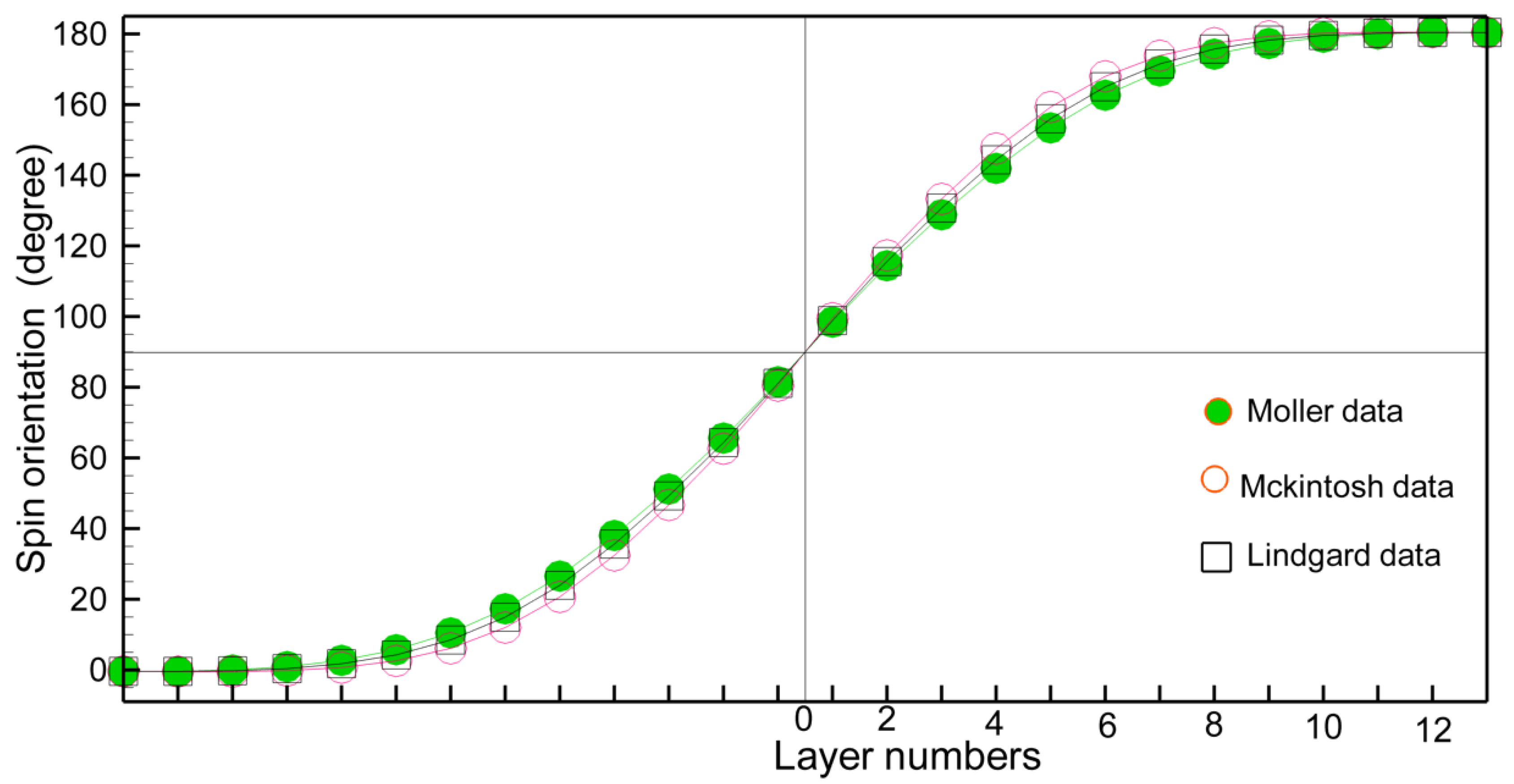
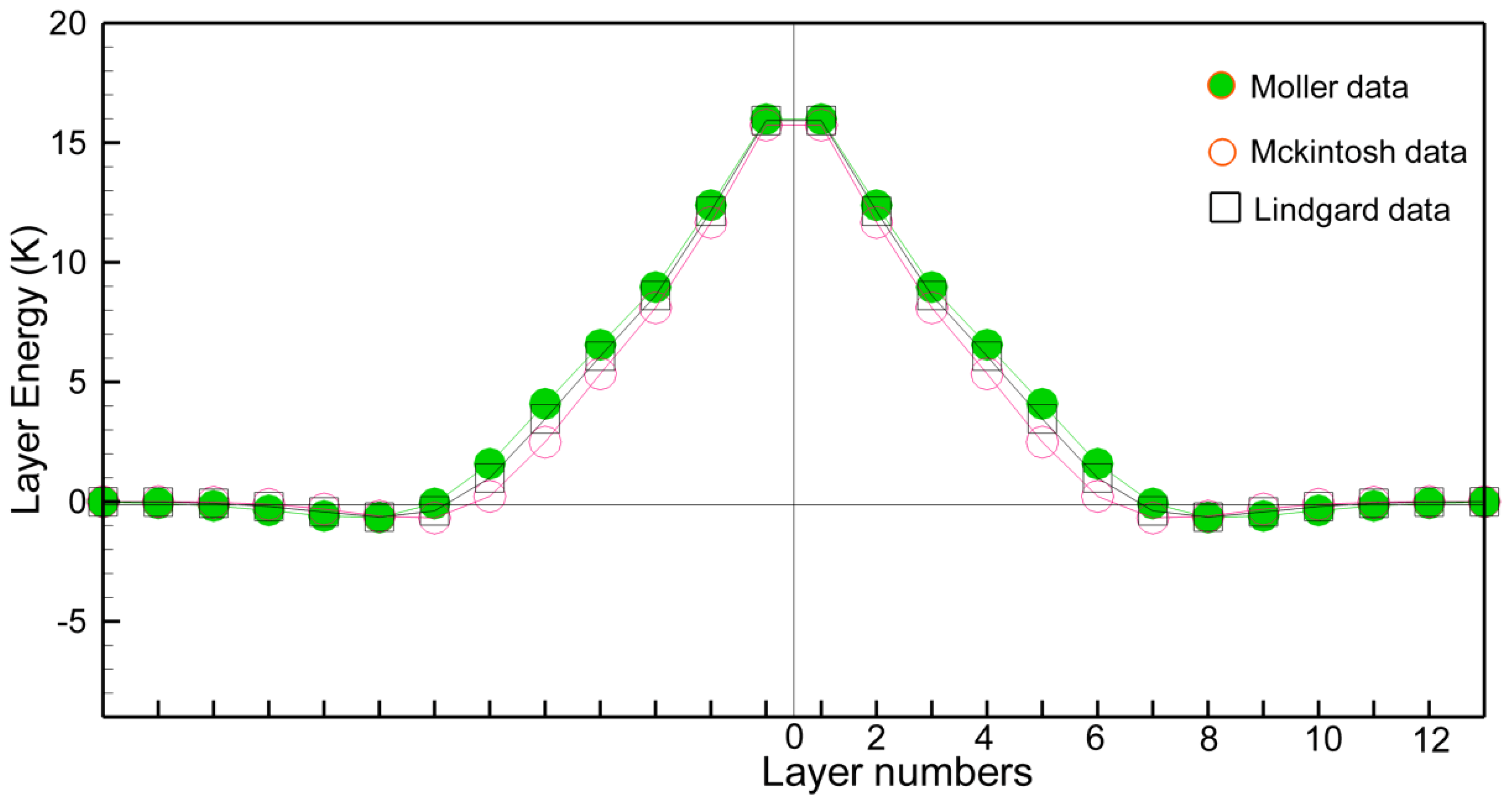
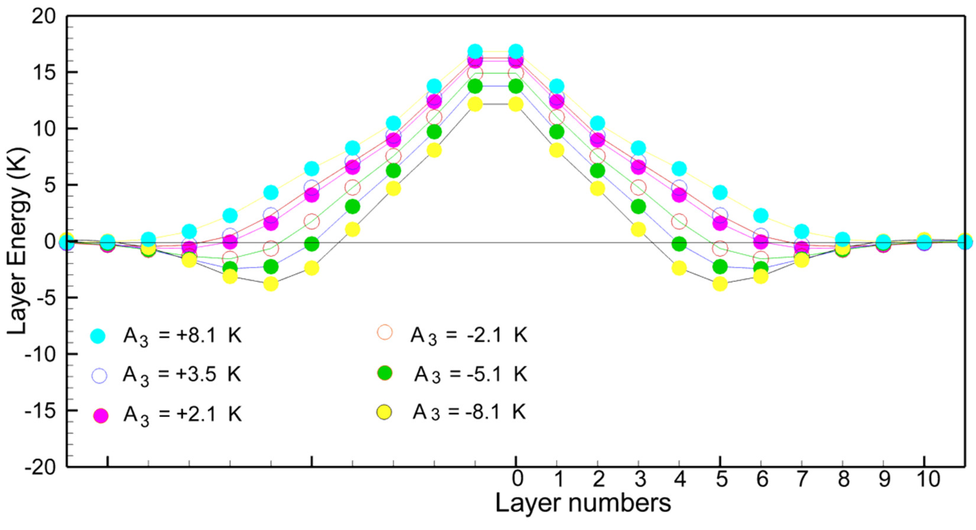
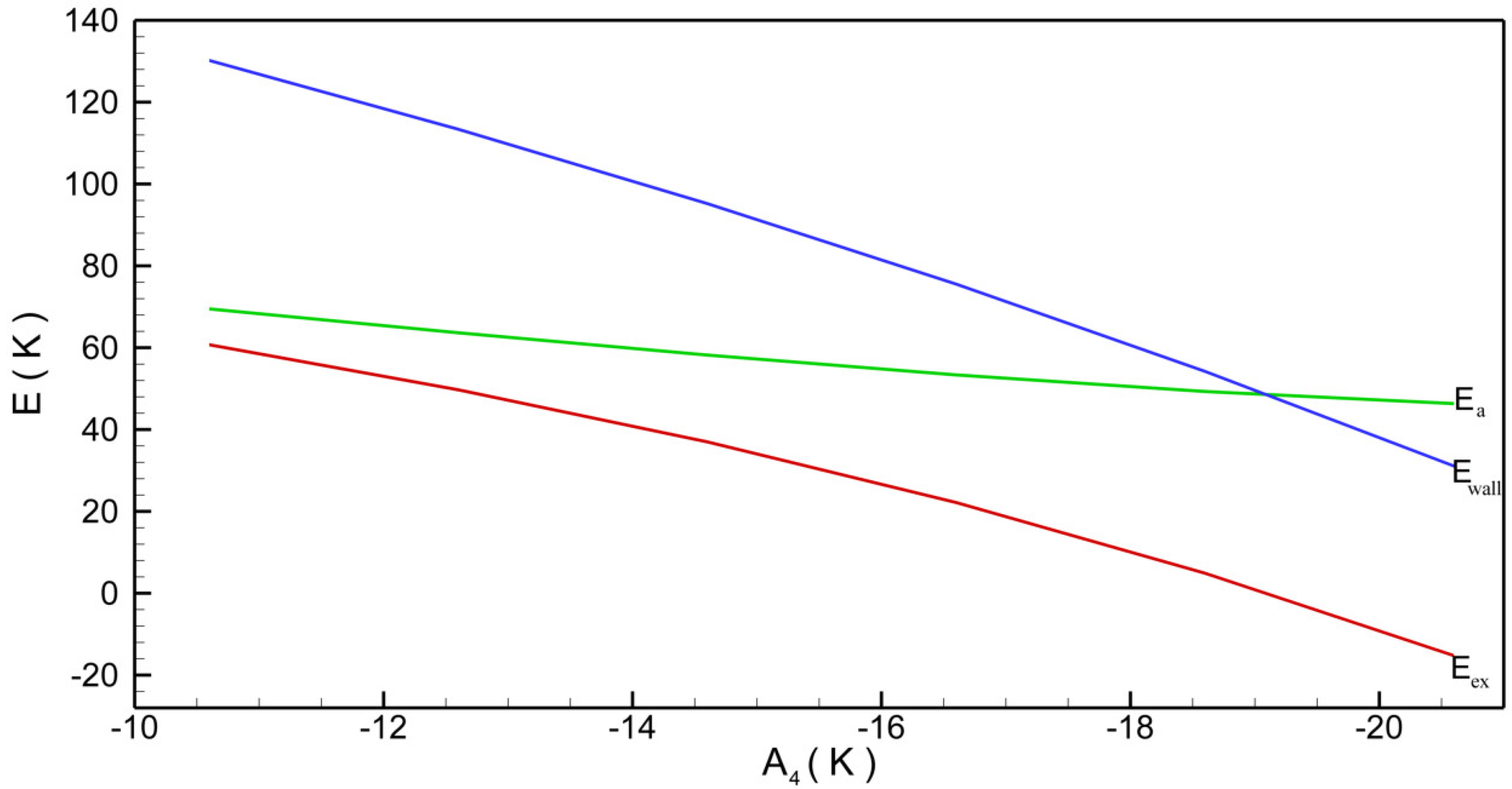
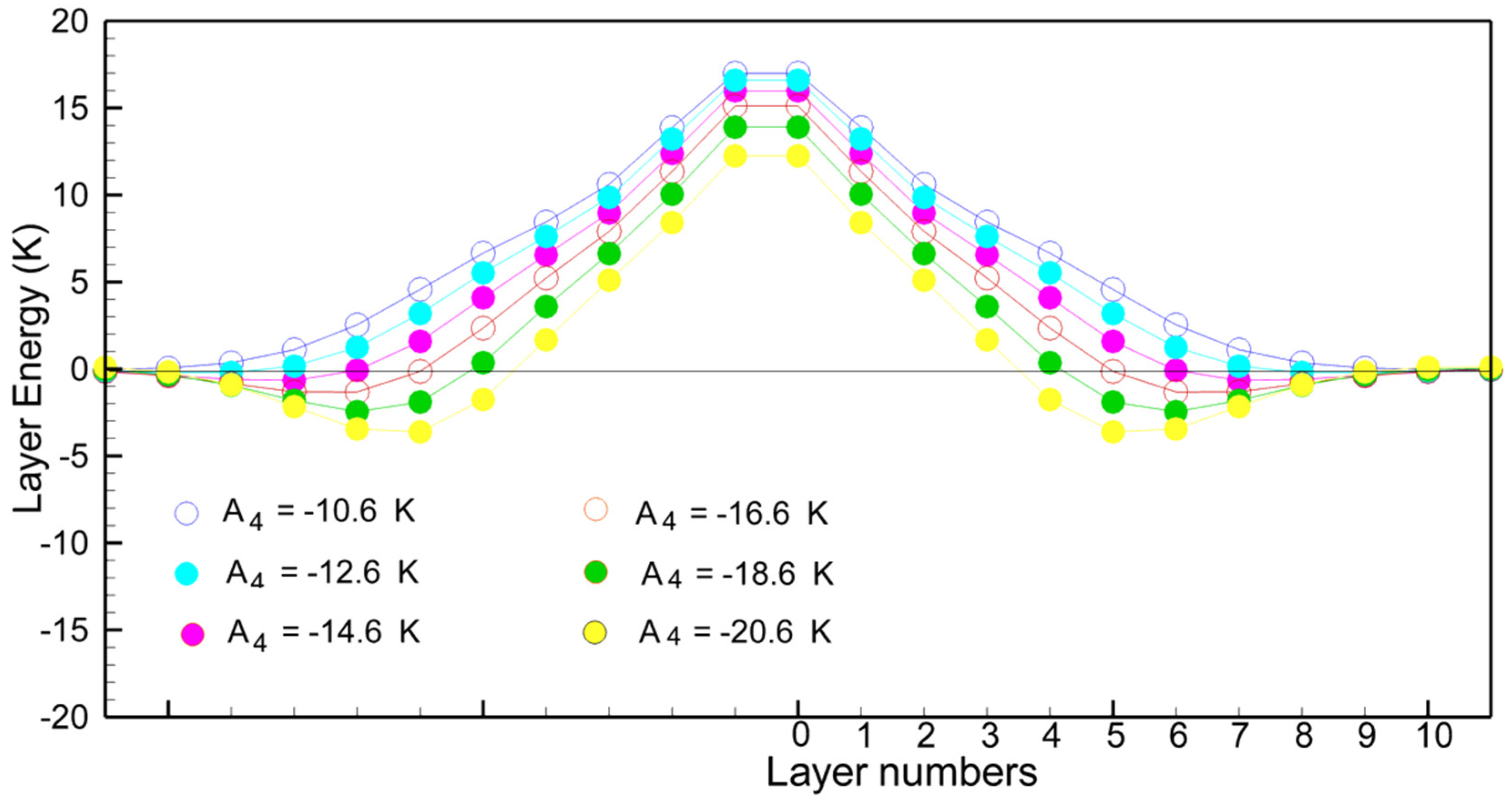
4. The Terbium Domain Wall
5. Some Remarks
6. Comment on the Bloch Wall
7. Conclusions
Author Contributions
Funding
Data Availability Statement
Acknowledgments
Conflicts of Interest
References
- Egami, T.; Graham, C.D., Jr. Domain walls in ferromagnetic Dy and Tb. J. Appl. Phys. 1971, 42, 1299. [Google Scholar] [CrossRef]
- Egami, T. Domain Walls in Ferromagnetic Dy. Ph.D. Dissertation, University of Pennsylvania, Philadelphia, PA, USA, 1971. [Google Scholar]
- Krause, S.; Berbil-Bautista, L.; Hanke, T.; Vonau, F.; Bode, M.; Wiesendanger, R. Consequences of line defects on the magnetic structure of high anisotropy films: Pinning centers on Dy/W(110). Europhys. Lett. 2006, 76, 637–643. [Google Scholar] [CrossRef]
- Berbil-Bautista, L.; Krause, S.; Bode, M.; Wiesendanger, R. Spin-polarized scanning tunneling microscopy and spectroscopy of ferromagnetic Dy(0001)/W(110) films. Phys. Rev. B 2007, 76, 064411. [Google Scholar] [CrossRef]
- Prieto, J.E.; Chen, G.; Schmid, A.K.; de la Figuera, J. Magnetism of epitaxial Tb films on W(110) studied by spin-polarized low-energy electron microscopy. Phys. Rev. B 2016, 94, 174445. [Google Scholar] [CrossRef]
- Chapman, J.N.; Morrison, G.R.; Fort, D.; Jones, D.W. An electron microscope investigation of domain structures in thin terbium foils. J. Magn. Magn. Mater. 1981, 22, 212–219. [Google Scholar] [CrossRef]
- Heigl, F.; Prieto, J.E.; Krupin, O.; Starke, K.; Kaindl, G. Annealing-induced extension of the antiferromagnetic phase in epitaxial terbium metal films. Phys. Rev. B 2005, 72, 035417. [Google Scholar] [CrossRef]
- Corner, D.W.; AI-Bassam, T.S. Magnetic domain structure of terbium single crystals. J. Phys. C Solid St. Phys. 1971, 4, 47–52. [Google Scholar] [CrossRef]
- Herring, C.P.; Jakubovics, J.P. Observation of magnetic domain patterns in terbium and dysprosium. J. Phys. F Met. Phys. 1973, 3, 157–160. [Google Scholar] [CrossRef]
- Corner, W.D.; Bareham, H.; Smith, R.L.; Saad, F.M.; Tanner, B.K.; Farrant, S.; Jones, D.W.; Beaudry, B.J.; Gschneidner, K.A. Magnetic domain structures in high purity single crystal terbium. J. Magn. Magn. Mater. 1980, 15–18, 1488–1490. [Google Scholar] [CrossRef]
- Morrison, G.R. The Observation of Magnetic Domain Structure in a Transmission Electron Microscope. Ph.D. Thesis, University of Glasgow, Glasgow, UK, 1981. [Google Scholar]
- Møller, H.B.; Houmann, J.C.G. Inelastic Scattering of Neutrons by Spin Waves in Terbium. Phys. Rev. Lett. 1966, 16, 737–739. [Google Scholar] [CrossRef]
- Moller, H.B.; Houmann, J.C.G.; Mackintosh, A.R. Magnetic Interactions in Tb and Tb-10% Ho from Inelastic Neutron Scattering. J. Appl. Phys. 1968, 39, 807–815. [Google Scholar] [CrossRef]
- Mackintosh, A.R.; Moller, H.B. Spin Waves. In Magnetic Properties of Rare Earth Metals; Elliott, R.J., Ed.; Springer: Greer, SC, USA, 1972; pp. 187–244. [Google Scholar]
- Lindgard, P.A. Spin waves in the heavy-rare-earth metals Gd, Tb, Dy, and Er. Phys. Rev. B 1978, 17, 2348. [Google Scholar] [CrossRef]
- Lindgard, P.A. Theory of Spin Excitations in the Rare Earth Systems. In Spin Waves and Magnetic Excitations; Modern Problems in Condensed Matter Sciences; Borovik-Romanov, A.S., Sinha, S.K., Eds.; North-Holland: Amsterdam, The Netherland, 1988; Volume 22, pp. 287–366. [Google Scholar]
- Stringfellow, M.W.; Holden, T.M.; Powell, B.M.; Woods, A.D.B. Spin waves in holmium. J. Phys. C Metal Phys. Suppl. 1970, 2, S189. [Google Scholar] [CrossRef]
- da Silva, A.F., Jr.; Mde Campos, F.; Martins, A.S. Domain wall structure in metals: A new approach to an old problem. J. Magn. Magn. Mater. 2017, 442, 236–241. [Google Scholar] [CrossRef]
- Van Den Broek, J.; Zijlstra, H. Calculation of intrinsic coercivity of magnetic domain walls in perfect crystals. IEEE Trans. Magn. 1971, 7, 226–230. [Google Scholar] [CrossRef]
- Kooy, C.; Enz, U. Experimental and theoretical study of the domain configuration in thin layers of BaFe_<12>O_<19>. Philips Res. Rep. 1960, 15, 7. [Google Scholar]
- Bloch, F. Zur Theorie des Austauschproblems und der Remanenzerscheinung der Ferromagnetika. Z. Für Phys. 1932, 74, 295–335. [Google Scholar] [CrossRef]
- Lilley, B.A. Energies and widths of domain boundaries in ferromagnetics. Phil. Mag. 1950, 41, 792–813. [Google Scholar] [CrossRef]
- Barbara, B. Louis Néel: His multifaceted seminal work in magnetism. Comptes Rendus Phys. 2019, 20, 631–649. [Google Scholar] [CrossRef]
- Scheie, A.; Laurell, P.; McClarty, P.A.; Granroth, G.E.; Stone, M.B.; Moessner, R.; Nagler, S.E. Spin-exchange Hamiltonian and topological degeneracies in elemental gadolinium. Phys. Rev. B 2022, 105, 104402. [Google Scholar] [CrossRef]
- Aharoni, A. Introduction to the Theory of Ferromagnetism; Oxford University Press: New York, NY, USA, 1996; p. 121. [Google Scholar]
- Hubert, A.; Schafer, R. The Analysis of Magnetic Microstructures. In Magnetic Domains, 3rd ed.; Springer: Berlin/Heidelberg, Germany, 1998; p. 203. [Google Scholar]
- Becker, R.; Doring, W. Ferromagnetismus; Springer: Berlin, Germany, 1939; p. 192. [Google Scholar]
- Enz, C.P. Heisenberg’s applications of quantum mechanics (1926–1933) or the settling of the new land. Helv. Phys. Acta 1983, 56, 993–1001. [Google Scholar]
- Locht, I.L.M.; Kvashnin, Y.O.; Rodrigues, D.C.M.; Pereiro, M.; Bergman, A.; Bergqvist, L.; Lichtenstein, A.I.; Katsnelson, M.I.; Delin, A.; Klautau, A.B.; et al. Standard model of the rare earths, analyzed from the Hubbard I approximation. Phys. Rev. B 2016, 94, 085137. [Google Scholar] [CrossRef]
- Goodings, D.A. Exchange interactions and the spin-wave spectrum of terbium. J. Phys. C (Proc. Phys. Soc.) 1968, 1, 125. [Google Scholar] [CrossRef]
- Jensen, J.; Mackintosh, A.R. Rare Earth Magnetism Structures and Excitations; Clarendon Press: Oxford, UK, 1991. [Google Scholar]
- Cooper, B.R. Magnetic properties of rare earth metals. Solid State Phys. 1968, 21, 393–490. [Google Scholar]
- Chapra, S.C.; Canale, R.P. Numerical Methods for Engineers; McGraw-Hill Education: New York, NY, USA, 2014. [Google Scholar]
- Rhyne, J.J.; Clark, A.E. Magnetic anisotropy of terbium and dysprosium. J. Appl. Phys. 1967, 38, 1379–1380. [Google Scholar] [CrossRef]
- Nicklow, R.M. SpinWave Dispersion Relation in RareEarth Metals. J. Appl. Phys. 1971, 42, 1672–1679. [Google Scholar] [CrossRef]
- Birss, R.R.; Keeler, G.J.; Shepherd, C.H. Temperature dependence of the magnetocrystalline anisotropy energy of terbium in the basal plane. J. Phys. F Met. Phys. 1977, 7, 1669–1681. [Google Scholar] [CrossRef]
- Ratnam, D.V.; Wells, R.G. Determination of Domain Wall Energies in Rare Earth Cobalt Compounds. AIP Conf. Proc. 1973, 10, 568. [Google Scholar] [CrossRef]
- Livingston, J.D.; McConnel, M.D. Domain-wall energy in cobalt-rare-earth compounds. J. Appl. Phys. 1972, 43, 4756–4762. [Google Scholar] [CrossRef]
- de Campos, M.F.; Romero, S.A.; de Castro, J.A. Estimation of texture and anisotropy field in a NdDyFeCoB magnet by magnetic measurements at the perpendicular direction. J. Magn. Magn. Mater. 2022, 564, 170119. [Google Scholar] [CrossRef]
- da Silva, A.F., Jr.; Martins, A.S.; de Campos, M.F. Spin glass transition in AuFe, CuMn, AuMn, AgMn and AuCr systems. J. Magn. Magn. Mater. 2019, 479, 222–228. [Google Scholar] [CrossRef]
- Furrer, A.; Podlesnyak, A.; Krämer, K.W. Extraction of exchange parameters in transition-metal perovskites. Phys. Rev. 2015, 92, 104415. [Google Scholar] [CrossRef]
- Wade R., H. The Determination of Domain Wall Thickness in Ferromagnetic Films by Electron Microscopy. Proc. Phys. Soc. 1962, 79, 1237. [Google Scholar] [CrossRef]
- Stoner, E.C.; Wohlfarth, E.P. A mechanism of magnetic hysteresis in heterogeneous alloys. IEEE Trans. Magn. 1991, 27, 3475–3518. [Google Scholar] [CrossRef]
- de Campos, M.F.; de Castro, J.A. Calculation of Recoil Curves in Isotropic and Anisotropic Stoner-Wohlfarth Materials. IEEE Trans. Magn. 2020, 56, 7512304. [Google Scholar] [CrossRef]
- Frei, E.H.; Shtrikman, S.; Treves, D. Critical Size and Nucleation Field of Ideal Ferromagnetic Particles. Phys. Rev. 1957, 106, 446–455. [Google Scholar] [CrossRef]
- de Campos, M.F. Achievements in micromagnetic techniques of steel plastic stage evaluation. Adv. Mater. Sci. 2020, 20, 16–55. [Google Scholar] [CrossRef]
- Döring, W. Point Singularities in Micromagnetism. J. Appl. Phys. 1968, 39, 1006. [Google Scholar] [CrossRef]
- Ruderman, M.A.; Kittel, C. Indirect Exchange Coupling of Nuclear Magnetic Moments by Conduction Electrons. Phys. Rev. 1954, 96, 99–102. [Google Scholar] [CrossRef]
- da Silva, A.F., Jr.; Martins, A.S.; de Campos, M.F. Longe Range Exchange Interactions in Sintered CuMn Alloys: A Monte Carlo Study. In Materials Science Forum; Trans Tech Publications, Ltd.: Bäch SZ, Switzerland, 2017; Volume 899, pp. 266–271. [Google Scholar] [CrossRef]
- da Silva, A.F.; Martins, A.S.; de Campos, M.F.; Lima, A.P. Revisiting Spin Glasses: Impact of Spin-Spin Interaction Range. Braz. J. Phys. 2018, 48, 39–45. [Google Scholar] [CrossRef]


| Exchange Term An | Moller [12,13] | Mckintosh [14] | Lindgard [15] |
|---|---|---|---|
| A1 | 127.4 | 112.4 | 121.6 |
| A2 | 31.3 | 30.1 | 35.9 |
| A3 | 2.1 | −4.2 | −0.4 |
| A4 | −14.6 | −15.5 | −20.0 |
| A5 | - | 3.3 | 3.8 |
Disclaimer/Publisher’s Note: The statements, opinions and data contained in all publications are solely those of the individual author(s) and contributor(s) and not of MDPI and/or the editor(s). MDPI and/or the editor(s) disclaim responsibility for any injury to people or property resulting from any ideas, methods, instructions or products referred to in the content. |
© 2024 by the authors. Licensee MDPI, Basel, Switzerland. This article is an open access article distributed under the terms and conditions of the Creative Commons Attribution (CC BY) license (https://creativecommons.org/licenses/by/4.0/).
Share and Cite
de Campos, M.F.; de Souza, K.S.T.; de Lima, I.R.; da Silva, C.C.; de Castro, J.A. Energy and Structure of the Terbium Domain Wall. Metals 2024, 14, 866. https://doi.org/10.3390/met14080866
de Campos MF, de Souza KST, de Lima IR, da Silva CC, de Castro JA. Energy and Structure of the Terbium Domain Wall. Metals. 2024; 14(8):866. https://doi.org/10.3390/met14080866
Chicago/Turabian Stylede Campos, Marcos F., Kaio S. T. de Souza, Ingrid R. de Lima, Charle C. da Silva, and Jose A. de Castro. 2024. "Energy and Structure of the Terbium Domain Wall" Metals 14, no. 8: 866. https://doi.org/10.3390/met14080866