
Investigation of Laser-Welded EH40 Steel Joint Stress with Different Thicknesses Based on a New Heat Source Model

Abstract
1. Introduction
2. Experiment
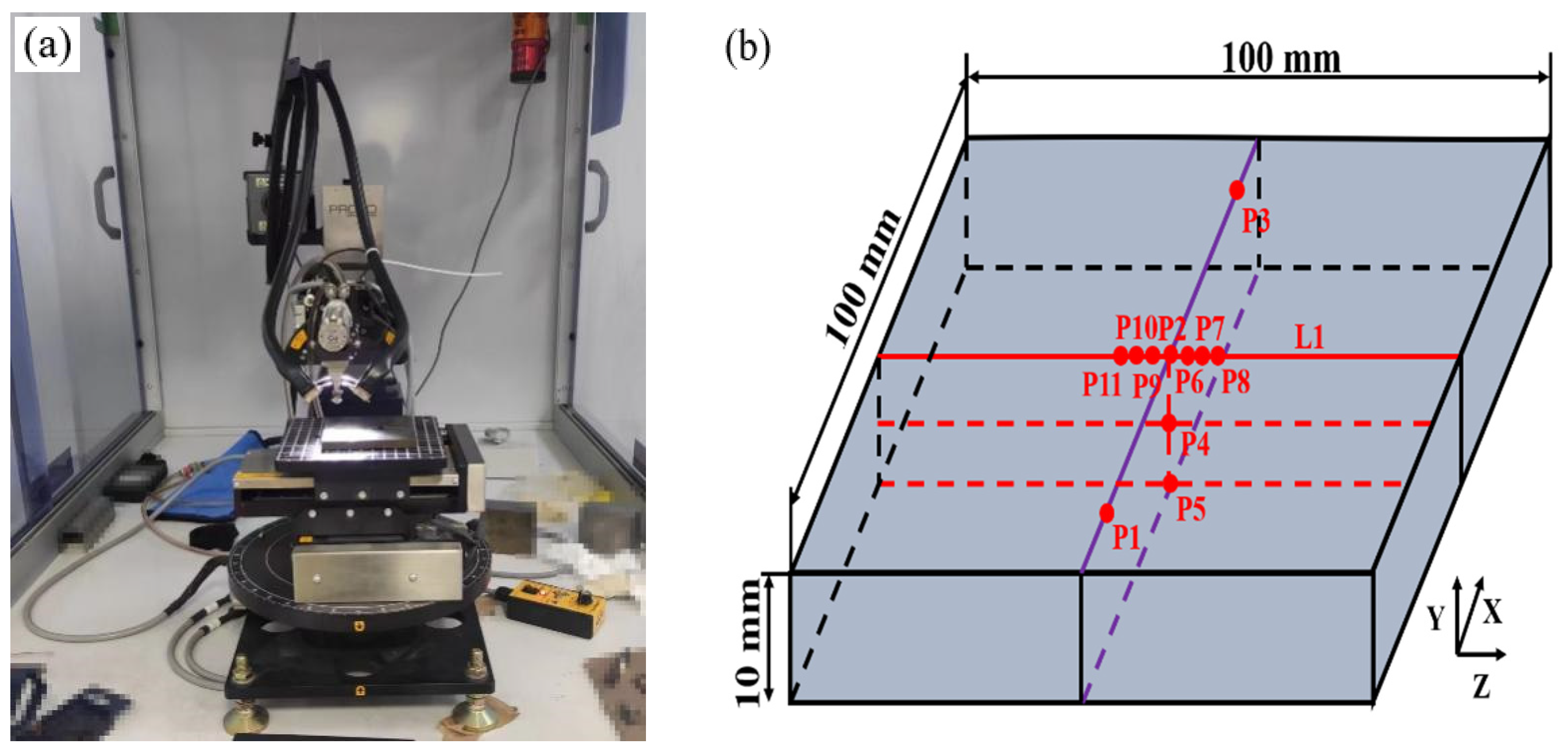
2.1. Welding and Measurement
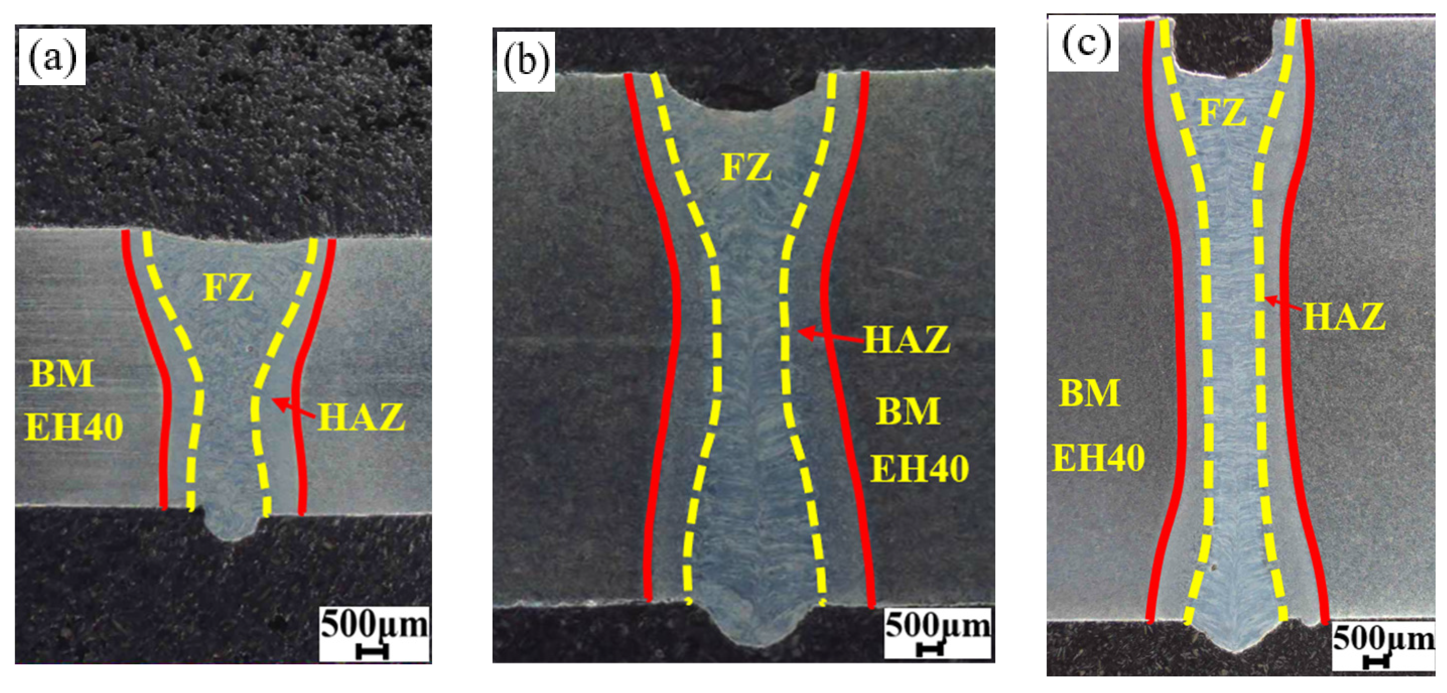
2.2. Weld Profile Analysis
3. Thermo-Mechanical Model and Numerical Simulation
3.1. New Heat Source Model and Theoretical Derivation
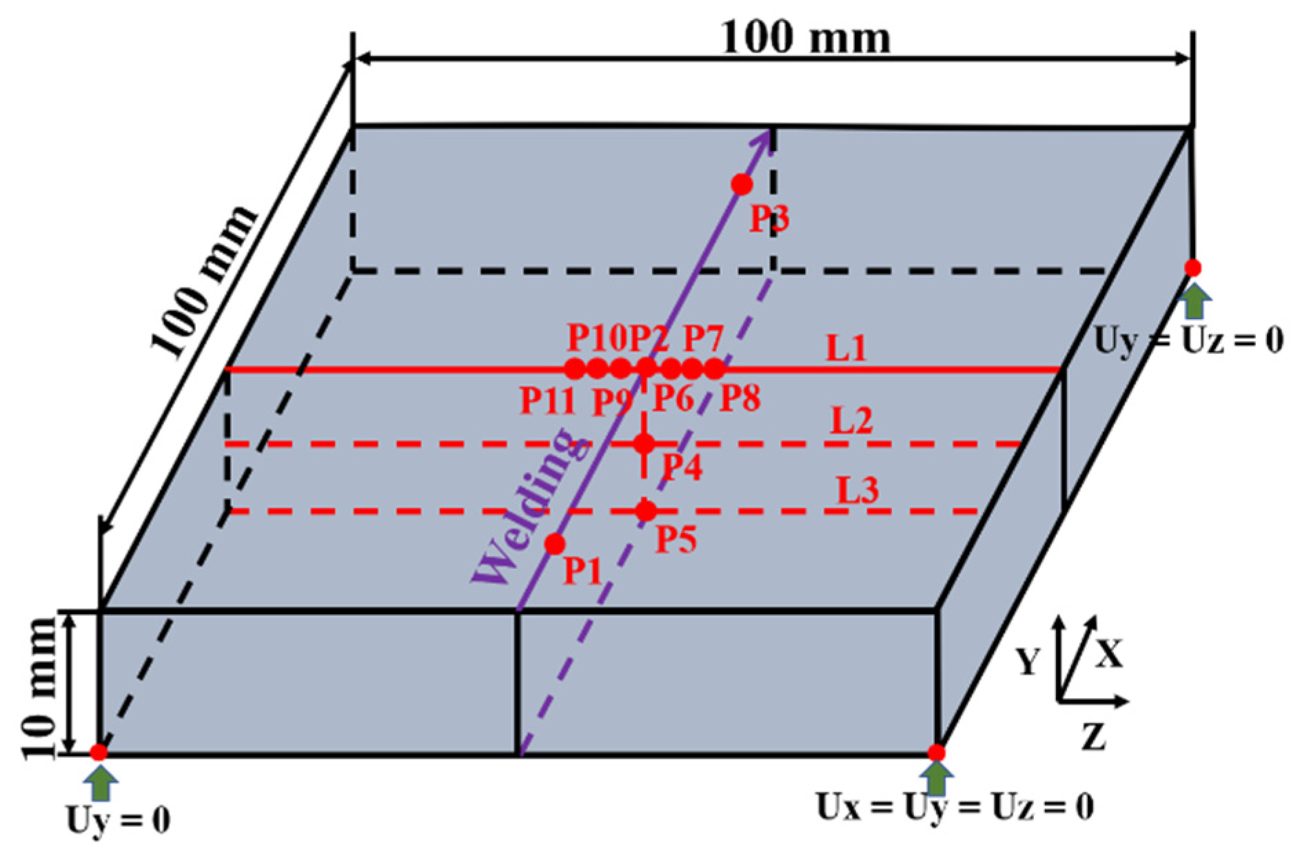
3.2. Mechanical Equilibrium Equation
3.3. Numerical Calculation Process
4. Results and Discussion
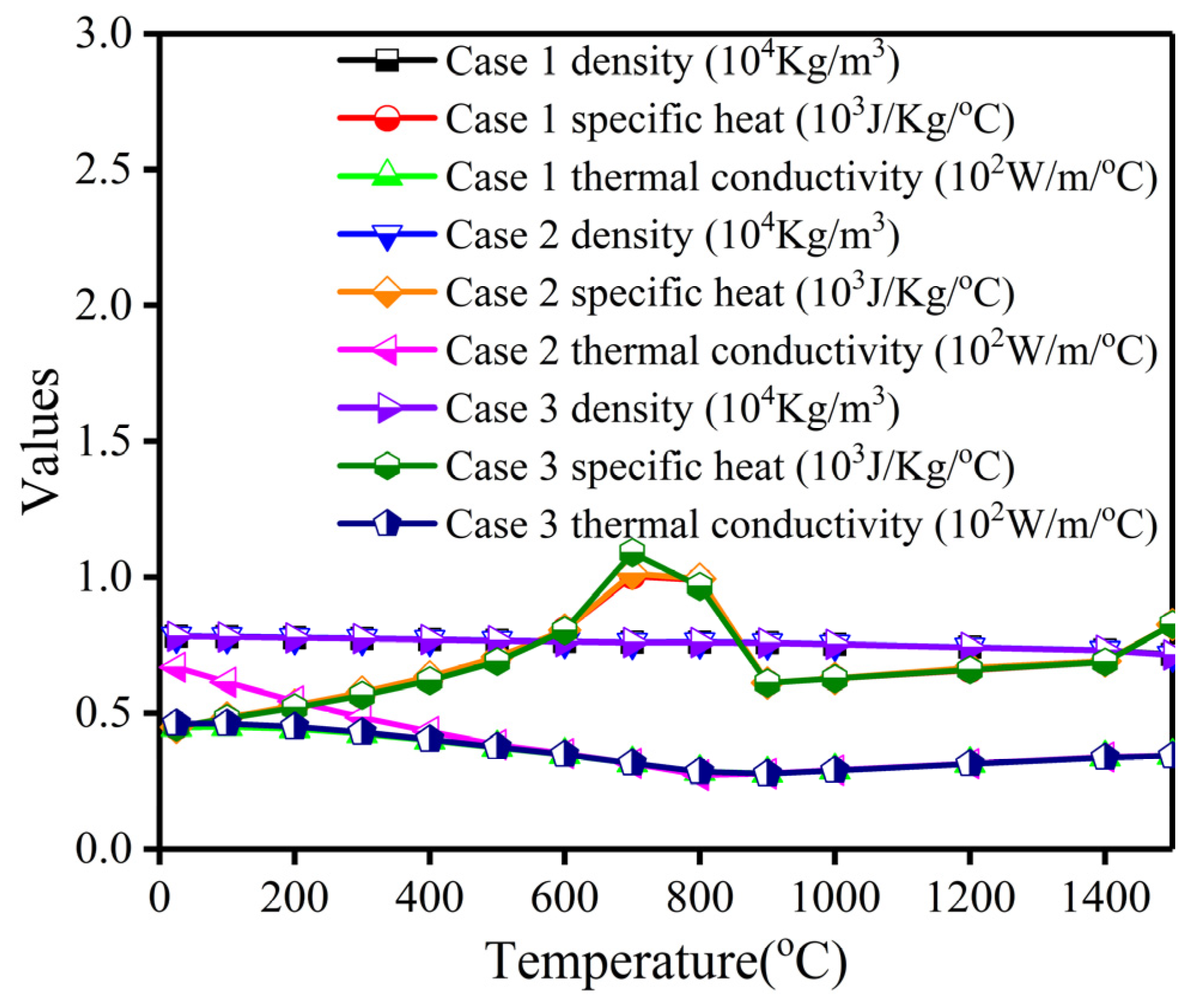
4.1. Thermal Analysis
4.2. Longitudinal Residual Stress Analysis
4.3. Transverse Residual Stress Analysis
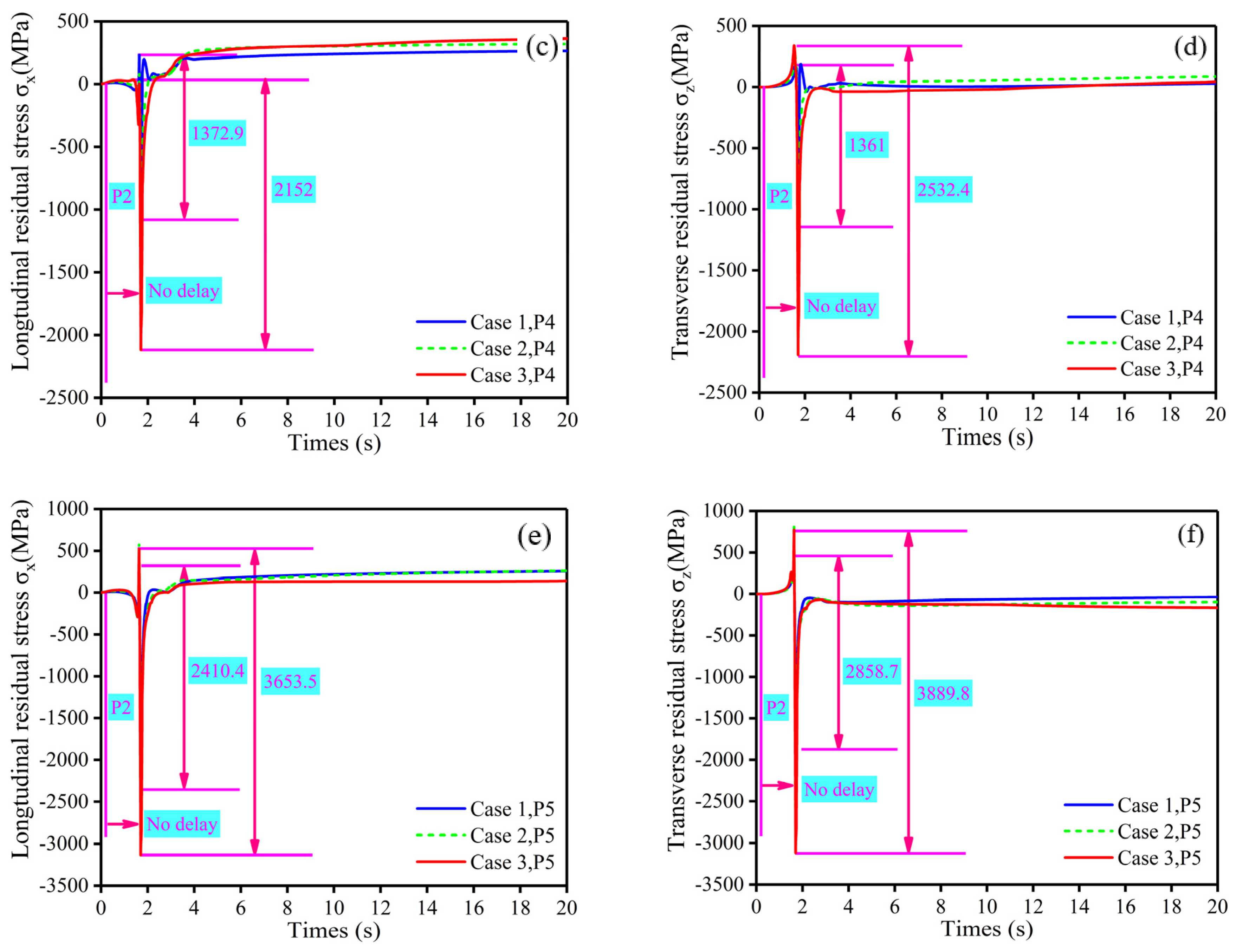
4.4. Stress Evolution Analysis
5. Conclusions
Author Contributions
Funding
Data Availability Statement
Conflicts of Interest
References
- Wu, R.L.; Huang, Y.; Xu, J.J.; Rong, Y.M.; Chen, Q.; Wang, L. Single-pass full penetration laser welding of 10-mm-thick EH40 using external magnetic field. J. Mater. Eng. Perform. 2022, 31, 9399–9410. [Google Scholar] [CrossRef]
- Zhan, X.H.; Liu, Y.; Liu, J.J.; Meng, Y.; Wei, Y.H.; Yang, J.K.; Liu, X.B. Comparative study on experimental and numerical investigations of laser beam and electron beam welded joints for Ti6Al4V alloy. J. Laser Appl. 2017, 29, 012020. [Google Scholar] [CrossRef]
- Qi, Y.; Chen, G.Y.; Deng, S.L.; Zhou, D.W. Root defects in full penetration laser welding of thick plates using steady electromagnetic force. J. Mater. Process. Technol. 2019, 273, 116247. [Google Scholar] [CrossRef]
- Friedrich, N. Experimental investigation on the influence of welding residual stresses on fatigue for two different weld geometries. Fatigue Fract. Eng. Mater. Struct. 2020, 43, 2715–2730. [Google Scholar] [CrossRef]
- Flores-Johnson, E.A.; Muránsky, O.; Hamelin, C.J.; Bendeich, P.J.; Edwards, L. Numerical analysis of the effect of weld-induced residual stress and plastic damage on the ballistic performance of welded steel plate. Comput. Mater. Sci. 2012, 58, 131–139. [Google Scholar] [CrossRef]
- Zhang, H.J.; Wang, Y.; Han, T.; Bao, L.L.; Wu, Q.; Gu, S.W. Numerical and experimental investigation of the formation mechanism and the distribution of the welding residual stress induced by the hybrid laser arc welding of AH36 steel in a butt joint configuration. J. Manuf. Process. 2020, 51, 95–108. [Google Scholar] [CrossRef]
- Liu, C.; Bing, W.; Jian, X.Z. Numerical investigation of residual stress in thick titanium alloy plate joined with electron beam welding. Metall. Mater. Trans. B 2010, 41, 1129–1138. [Google Scholar] [CrossRef]
- Wang, J.Q.; Han, J.M.; Domblesky, J.; Yang, Z.Y.; Zhao, Y.X.; Zhang, Q. Development of a new combined heat source model for welding based on a polynomial curve fit of the experimental fusion line. Int. J. Adv. Manuf. Technol. 2016, 87, 1985–1997. [Google Scholar] [CrossRef]
- Farrokhi, F.; Endelt, B.; Kristiansen, M. A numerical model for full and partial penetration hybrid laser welding of thick-section steels. Opt. Laser Technol. 2018, 111, 671–686. [Google Scholar] [CrossRef]
- Wu, C.S.; Hu, Q.X.; Gao, J.Q. An adaptive heat source model for finite-element analysis of keyhole plasma arc welding. Comput. Mater. Sci. 2009, 46, 167–172. [Google Scholar] [CrossRef]
- Li, Y.; Feng, Y.H.; Zhang, X.X.; Wu, C.S. An improved simulation of heat transfer and fluid flow in plasma arc welding with modified heat source model. Int. J. Mech. Sci. 2013, 64, 93–104. [Google Scholar] [CrossRef]
- Kik, T. Heat source models in numerical simulations of laser welding. Materials 2020, 13, 2653. [Google Scholar] [CrossRef] [PubMed]
- Liu, J.Z.; Zhan, X.H.; Gao, Z.N.; Yan, T.Y.; Zhou, Z.H. Microstructure and stress distribution of TC4 titanium alloy joint using laser-multi-pass-narrow-gap welding. Int. J. Adv. Manuf. Technol. 2020, 108, 3725–3735. [Google Scholar] [CrossRef]
- Fang, J.X.; Li, S.; Dong, S.; Wang, Y.; Huang, H.; Jiang, Y.; Liu, B. Effects of phase transition temperature and preheating on residual stress in multi-pass & multi-layer laser metal deposition. J. Manuf. Process. 2021, 68, 1585. [Google Scholar]
- Chen, L.; Mi, G.Y.; Zhang, X.; Wang, C.M. Numerical and experimental investigation on microstructure and residual stress of multi-pass hybrid laser-arc welded 316L steel. Mater. Des. 2019, 168, 107653. [Google Scholar] [CrossRef]
- Li, H.H.; Dai, W.; Huang, Y.; Yan, W.; Wu, R.L.; Wang, D. Numerical and experimental study on thermal-metallurgical-mechanical behavior of high-strength steel welded joint. Opt. Laser Technol. 2024, 175, 110802. [Google Scholar] [CrossRef]
- Pu, X.W.; Zhang, C.H.; Li, S.; Deng, D. Simulating welding residual stress and deformation in a multi-pass butt-welded joint considering balance between computing time and prediction accuracy. Int. J. Adv. Manuf. Technol. 2017, 93, 2215–2226. [Google Scholar] [CrossRef]
- Jiang, J.H.; Zeng, W.S.; Li, L.B. Effect of residual stress on hydrogen diffusion in thick butt-welded high-strength steel plates. Metals 2022, 12, 1074. [Google Scholar] [CrossRef]
- Ghafouri, M.; Ahola, A.; Ahn, J.; Björk, T. Welding-induced stresses and distortion in high-strength steel T-joints: Numerical and experimental study. J. Constr. Steel Res. 2022, 189, 107088. [Google Scholar] [CrossRef]
- Lee, C.H.; Chang, K.H. Temperature fields and residual stress distributions in dissimilar steel butt welds between carbon and stainless steels. Appl. Therm. Eng. 2012, 46, 33–41. [Google Scholar] [CrossRef]
- Gao, S.; Geng, S.N.; Jiang, P.; Han, C.; Ren, L.Y. Numerical study on the effect of residual stress on mechanical properties of laser welds of aluminum alloy 2024. Opt. Laser Technol. 2022, 146, 10758. [Google Scholar] [CrossRef]
- Rong, Y.M.; Huang, Y.; Xu, J.J.; Zheng, H.J.; Zhang, G.J. Numerical simulation and experiment analysis of angular distortion and residual stress in hybrid laser-magnetic welding. J. Mater. Process. Technol. 2017, 245, 270–277. [Google Scholar] [CrossRef]
- Mato, P.; Ivica, G.; Zdenko, T.; Tomaž, V.; Sandro, N.; Hrvoje, D. Numerical prediction and experimental validation of temperature and residual stress distributions in buried-arc welded thick plates. Int. J. Energy Res. 2019, 43, 3590–3600. [Google Scholar]
- Sun, G.F.; Wang, Z.D.; Lu, Y.; Zhou, R.; Ni, Z.H.; Gu, X.; Wang, Z.G. Numerical and experimental investigation of thermal field and residual stress in laser-MIG hybrid welded NV E690 steel plates. J. Manuf. Process. 2018, 34, 106–120. [Google Scholar] [CrossRef]
- Wu, R.L.; Huang, Y.; Xu, J.J.; Rong, Y.M.; Chen, Q. Stress and distortion of the 10 mm thick plate EH40 and 316L different butt joints in 10 kW laser welding. Opt. Laser Technol. 2022, 152, 108179. [Google Scholar] [CrossRef]
- Zhang, H.J. Research on Temperature Field and Residual Stress During Laser Flat Plate Welding; Changchun University of Science and Technology: Changchun, China, 2016. [Google Scholar]
- Wang, J.; Shibahara, M.; Zhang, X.; Murakawa, H. Investigation on twisting distortion of thin plate stiffened structure under welding. J. Mater. Process. Technol. 2012, 212, 1705–1715. [Google Scholar] [CrossRef]
- Banik, S.D.; Kumar, S.; Singh, P.K.; Bhattacharya, S.; Mahapatra, M.M. Distortion and residual stresses in thick plate weld joint of austenitic stainless steel: Experiments and analysis. J. Mater. Process. Technol. 2021, 289, 116–944. [Google Scholar] [CrossRef]
- Xie, J.L.; Ma, Y.C.; Wang, M.; Li, H.Z.; Fang, N.; Liu, K. Interfacial characteristics and residual welding stress distribution of K4750 and Hastelloy X dissimilar superalloys joints. J. Manuf. Process. 2021, 67, 253–261. [Google Scholar] [CrossRef]
- Ahn, J.; He, E.; Chen, L.; Wimpory, C.; Dear, J.P.; Davies, C.M. Prediction and measurement of residual stresses and distortions in fibre laser welded Ti-6Al-4V considering phase transformation. Mater. Des. 2017, 115, 441–457. [Google Scholar] [CrossRef]
- Ahmad, N.M.; Geng, P.H.; Wu, C.S.; Ma, N. Unravelling the ultrasonic effect on residual stress and microstructure in dissimilar ultrasonic-assisted friction stir welding of Al/Mg alloys. Int. J Mach. Tool Manuf. 2023, 186, 104004. [Google Scholar]


| C | Si | Mn | P | S | Cu | Cr | |
| 6 mm | 0.10 | 0.26 | 1.53 | 0.012 | 0.002 | 0.02 | 0.02 |
| 10 mm | 0.141 | 0.16 | 1.45 | 0.019 | 0.005 | 0.01 | 0.017 |
| 15 mm | 0.12 | 0.31 | 1.36 | 0.018 | 0.004 | 0.02 | 0.04 |
| Ni | Nb | V | Ti | Mo | Al | Fe | |
| 6 mm | 0.01 | 0.027 | 0.005 | 0.013 | 0.003 | 0.029 | Bal. |
| 10 mm | 0.007 | 0.041 | 0.004 | 0.017 | 0.002 | 0.027 | Bal. |
| 15 mm | 0.02 | 0.01 | 0.003 | 0.012 | 0 | 0.021 | Bal. |
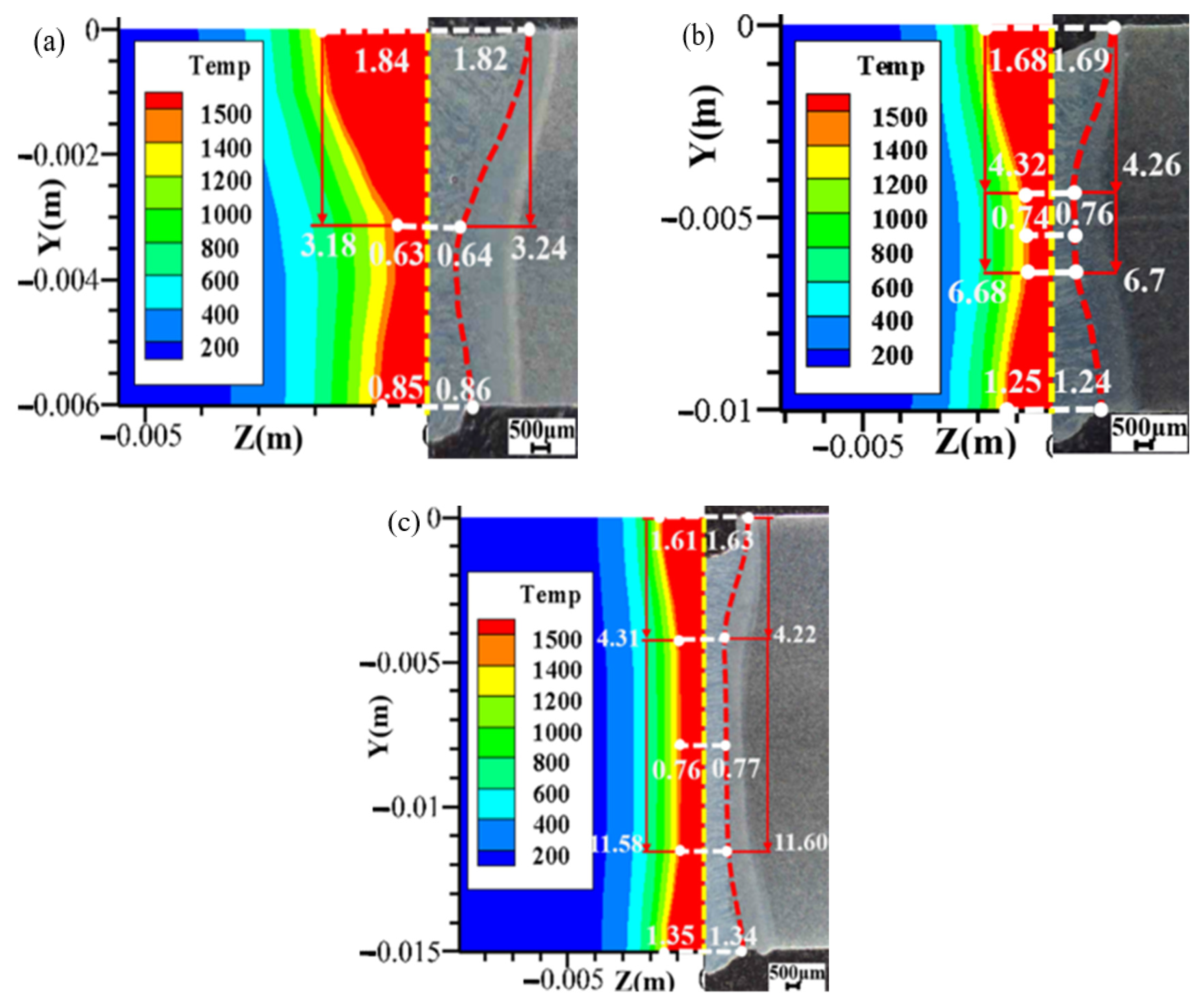
| Parameters | Item | Case 3 | DC Model [9] |
|---|---|---|---|
| rt (mm) | Experiment | 1.63 | 1.63 |
| Simulation | 1.61 | 1.88 | |
| Errors Δ (%) | −1.23 | 15.3 | |
| zi1 (mm) | Experiment | 4.22 | - |
| Simulation | 4.31 | - | |
| Errors Δ (%) | 2.13 | - | |
| ri (mm) | Experiment | 0.77 | 0.77 |
| Simulation | 0.76 | 0.84 | |
| Errors Δ (%) | −1.3 | 9.09 | |
| zi2 (mm) | Experiment | 11.60 | - |
| Simulation | 11.58 | - | |
| Errors Δ (%) | −0.17 | - | |
| rb (mm) | Experiment | 1.34 | 1.34 |
| Simulation | 1.35 | 1.38 | |
| Errors Δ (%) | 0.75 | 2.98 |
Disclaimer/Publisher’s Note: The statements, opinions and data contained in all publications are solely those of the individual author(s) and contributor(s) and not of MDPI and/or the editor(s). MDPI and/or the editor(s) disclaim responsibility for any injury to people or property resulting from any ideas, methods, instructions or products referred to in the content. |
© 2025 by the authors. Licensee MDPI, Basel, Switzerland. This article is an open access article distributed under the terms and conditions of the Creative Commons Attribution (CC BY) license (https://creativecommons.org/licenses/by/4.0/).
Share and Cite
Wu, R.; Wu, X.; Hu, S.; He, C.; Li, H.; Liu, Y. Investigation of Laser-Welded EH40 Steel Joint Stress with Different Thicknesses Based on a New Heat Source Model. Metals 2025, 15, 188. https://doi.org/10.3390/met15020188
Wu R, Wu X, Hu S, He C, Li H, Liu Y. Investigation of Laser-Welded EH40 Steel Joint Stress with Different Thicknesses Based on a New Heat Source Model. Metals. 2025; 15(2):188. https://doi.org/10.3390/met15020188
Chicago/Turabian StyleWu, Ruolin, Xingyu Wu, Shuai Hu, Chaomei He, Huanhuan Li, and Yuan Liu. 2025. "Investigation of Laser-Welded EH40 Steel Joint Stress with Different Thicknesses Based on a New Heat Source Model" Metals 15, no. 2: 188. https://doi.org/10.3390/met15020188
APA StyleWu, R., Wu, X., Hu, S., He, C., Li, H., & Liu, Y. (2025). Investigation of Laser-Welded EH40 Steel Joint Stress with Different Thicknesses Based on a New Heat Source Model. Metals, 15(2), 188. https://doi.org/10.3390/met15020188