Research on Performance Prediction Method of Refractory High-Entropy Alloy Based on Ensemble Learning

Abstract

Due to the huge component space of refractory high-entropy alloy, the traditional, experimental “trial and error method” can not meet the design requirements. In order to improve the “trial and error method”, guidance is provided for the prediction and design of refractory high-entropy alloys. Based on the literature data, a comprehensive dataset was constructed, including the composition, phase composition, and strength data of various high-entropy alloys. On this basis, nine regression models were established for strength prediction. By comparison, the XGBoost (XGB) model achieves better prediction performance in the test set; the root mean square error (RMSE) is 195.53 MPa, and the coefficient of determination (R²) is 0.87. By using Shapley additive interpretation (SHAP) to analyze the explainability of the model, it was found that the key characteristics affecting the mechanical properties of the high-entropy alloy were mixed entropy and electronegativity. In order to further evaluate the precision of the model, through the vacuum arc melting preparation, Ti27.5Zr26.5Nb25.5Ta8.5Al12 high-entropy alloys were experimentally verified. The alloy experiments’ yield strength was 1356 MPa, predicting strength was 1304.71 MPa, external validation error was 3.81%, and the average accuracy of the model was 87.38%.

1. Introduction

With the rapid development of aerospace, petrochemical, gas turbine, and other fields, more stringent requirements have been put forward for the performance of high-temperature metal materials [1,2,3]. Due to the inherent limitation of the melting point of materials, the temperature resistance of traditional nickel-based superalloys is close to the limit, but it still cannot meet the performance requirements of nuclear reactors, liquid rocket engine nozzles, gas turbine blades, and other components in ultra-high temperatures and extreme environments [4]. Therefore, it is urgent to design metal materials with better performance at high temperatures. High-entropy alloys (HEAs), as a novel and promising candidate, have attracted extensive attention in recent years. HEAs are defined as multi-principal-element alloys (typically ≥5 elements) with near-equimolar compositions, which exhibit a unique “high-entropy effect”—the significant increase in configurational entropy stabilizes simple solid solution phases (e.g., BCC or FCC) instead of intermetallic compounds, thereby enhancing mechanical properties and thermal stability.

The paradigm shift from traditional alloys to HEAs was first demonstrated by Senkov et al. [5], who synthesized two refractory high-entropy alloys (RHEAs), NbMoTaW and NbMoTaVW, by incorporating refractory elements (V, Cr, Zr, Nb, Hf, Mo, and W). RHEAs leverage both the high-entropy effect and the inherent high melting points of refractory metals to achieve exceptional strength retention above 1000 °C. However, most RHEAs suffer from a limited room-temperature ductility (compressive fracture strain <10%) due to severe lattice distortion and dislocation pinning effects, posing a critical challenge for their processing and engineering applications [6,7,8,9,10,11].

To address this challenge, researchers have explored composition design strategies for balancing strength and ductility. For example, Han et al. [12] improved the strength-ductility trade-off in TiNbMoTaW(V) by optimizing Ti content, while Juan et al. [13] enhanced the high-temperature yield stress of TaNbHfZrTi through Mo addition. Despite these advances, traditional trial-and-error approaches remain inefficient in navigating the vast compositional space of RHEAs (≥5 elements with 5–35% atomic ratios), often relying on empirical intuition rather than quantitative design principles.

Some researchers have proposed important design criteria for high-entropy alloys that partially address this problem. For example, Singh et al. [14] have proposed a dimensionless measure of quantum mechanics, local lattice distortion (LLD), as a reliable predictor of ductility. The LLD expression includes electronegativity differences in the local chemical environment, as well as atomic-scale shifts due to local lattice distortions and weighted averages of valence electron counts. When the LLD is less than 0.3, the alloy is considered ductile; otherwise, it is considered a brittle material. Guo et al. [15] studied the effect of valence electron concentration (VEC) on the formation of high-entropy alloy phases. When the VEC is greater than 8.0, an FCC phase occurs. When the VEC is less than 6.87, a BCC phase occurs. When the VEC is between 6.87 and 8.0, there is a mixed phase of FCC and BCC. By adjusting the ratio of the FCC and BCC phases, the strength and plasticity of the material can be altered. However, these criteria still have some shortcomings for refractory high-entropy alloys: (1) LLD does not consider the temperature-dependent dislocation dynamics. (2) VEC cannot account for the non-equal atomic ratio components commonly found in RHEAs. (3) Neither of the two criteria achieves multi-performance optimization (such as synergistic improvement of strength and plasticity).

In recent years, with the rapid development of data-driven technology and machine learning algorithms, machine learning has been widely applied in all aspects of materials science, including component design, material preparation process, mechanism research, etc. [16,17,18,19,20,21,22].

Machine learning is data-centric, by using specific algorithms to search and learn the data, and then extract the key knowledge information in the data, and use it to guide the efficient design of alloy components. Klimenko et al. [23] constructed a support vector machine (SVM)-based proxy model to predict the yield strength of refractory high-entropy alloys of an Al-Cr-Nb-Ti-V-Zr system at different temperatures (20 °C, 600 °C, and 800 °C). Firstly, data of the alloy yield strength at different temperatures were collected, and datasets were established. Based on literature analysis, features related to solid solution strengthening and phase formation of the alloys were selected, such as atomic radius difference, valence electron concentration, and mixing enthalpy, etc. Meanwhile, redundant features were removed by Pearson correlation analysis to optimize the feature set. By comparing seven machine learning algorithms, the radial basis function kernel of support vector regression (SVR-RBF) is selected as the optimal algorithm, and its hyperparameters are optimized by grid search and root mean square error (RMSE). In the process of model training, the bootstrap method and cross-validation method are used to verify the prediction accuracy of the model, and bagging technology is used to further improve the prediction accuracy. Ultimately, the model showed a high prediction accuracy at 20 °C and 600 °C (error of 7% and 12%, respectively), but the error increased significantly at 800 °C (error of more than 20%), which may be related to the transition of the alloy from a non-thermal platform to a strong temperature dependence at that temperature. Machine learning methods helped researchers better understand the relationship between alloy composition and material parameters and mechanical properties. However, the current research mainly focuses on yield strength and plasticity, but few people study the multi-objective optimization for improving yield strength and plasticity at the same time.

In this paper, a comprehensive dataset comprising 652 pieces of refractory high-entropy alloy data was meticulously integrated from the literature. Unlike most existing studies that rely solely on their own experimental data for machine learning, which often results in a limited data volume and a relatively homogeneous system, our research stands out by sourcing data from a diverse range of 90 different publications. This approach not only ensures a substantial dataset but also enriches the diversity of high-entropy alloy systems, thereby providing a more robust and versatile foundation for model training. After systematic data preprocessing and feature screening, 17 features were obtained for training 9 different models. In order to ensure the fairness of evaluation, the hybrid parameter tuning method combining grid search and Bayes optimization is used to obtain the best hyperparameters for all models. The SHapley Additive exPlanations method is used to analyze the model, improving the transparency and interpretability of the model. Finally, we selected the eXtreme Gradient Boosting (XGB) model as the prediction model for the mechanical properties of the high-entropy alloy and obtained the parameters’ mixing entropy (ΔS) and electronegativity difference (μ) that had the greatest influence on the model properties.

2. Material and Methods

2.1. Data Acquisition and Preprocessing

Machine learning is a data-driven approach where data quality and quantity significantly impact model accuracy. The dataset for this study’s refractory high-entropy alloy prediction model for mechanical properties comes from published relevant articles. It includes 655 data entries covering composition (elements like Ti, V, Zr, Nb, Mo, Hf, etc.), physical properties (density and melting point), thermodynamic parameters (mixing enthalpy and atomic size difference), and mechanical properties (yield strength and fracture strain). A systematic data preprocessing procedure was adopted to ensure data quality.

2.1.1. Data Preprocessing

(1)

Outlier Sample Elimination

For non-numerical features, analyze their distributions. In the testing type (TM) feature, 652 samples are compression tests, and only 3 are tension tests (0.46%). Considering the small sample size of the tension test and the essential stress difference from compression tests, the tension test samples are identified as outliers using the 3σ rule and removed.

(2)

High Missing-Value Feature Processing

From materials science knowledge, processing technology greatly affects mechanical properties. In this dataset, the maximum yield strength of unprocessed refractory high-entropy alloys is 2390 Mpa. After processing, it can reach up to 3416 Mpa, a 42.93% increase. However, the processing condition (cast conditions) feature has a missing rate of 90.99%, making it hard to establish an effective mapping relationship. Thus, to avoid noise, this feature is deleted. The missing rate of Smax is 72.3%, way above the usual feature selection threshold. In engineering, yield strength is key for structural material design, while Smax is more for failure analysis. So, deleting the Smax feature is reasonable.

(3)

Redundant feature processing

The phases feature has 67 distinct values, 81.2% of which are BCC-related. With a high cardinality problem, one-hot encoding would cause dimension explosion. One-hot encoding is converting categorical data into a binary matrix, with each category as a column marked by 1 s and 0 s. This dimension explosion exacerbates data sparsity and overfitting risks in training. Also, the uneven sample distribution (over 80% BCC) weakens the model’s learning ability. Given insufficient samples, feature space expansion, and data quality issues, the phases feature cannot reliably support mechanical property prediction. Consequently, this feature was excluded from further analysis.

(4)

Stress type standardization

Feature E/T indicates the type of stress–strain representation of the data, E indicates the engineering stress–strain used, and T indicates the true stress–strain used. The real stress–strain and engineering stress–strain can be converted, and the yield strength (YS) can be unified into the value of engineering stress through conversion, which ensures the unity of a yield strength measurement. The specific formula is as follows:

$${\sigma }_T={\sigma }_E(1+\epsilon )$$

(1)

where σ_T represents true stress, σ_E represents engineering stress, and ε represents strain.

(5)

Data filling

For the numerical features, statistical analysis shows that the difference between the median and mean is very small, and the data is highly intact. In this case, the median imputation has several advantages. First, the median is naturally robust to outliers and can avoid the interference of abnormal data in the imputation results. Second, when the missing rate is low, the difference between median and mean imputation is negligible. Finally, median imputation best preserves the original data distribution. The Kolmogorov–Smirnov test, which assesses the similarity between two distributions by analyzing the maximum difference between their cumulative distribution functions, indicates that the imputed features maintain a similarity of over 94.6% to the original data distribution. Considering data integrity, computational efficiency, and distribution preservation, we ultimately selected the median as the missing value imputation method.

2.1.2. Feature Screening

Considering that there are many types of data and the amount of data is limited, it is difficult for the direct training model to achieve better prediction accuracy. There is a certain linear relationship between the characteristic parameters of high-entropy alloys, so it is important to study the correlation degree and find out the parameters with a high repetition for the subsequent model training. The Pearson correlation coefficient is defined as the quotient of the product of the covariance and standard deviation between two variables and is often used to measure the degree of linear correlation between two variables. In this paper, the Pearson correlation coefficient is used to measure the linear relationship between features and features and between features and targets. Figure 1 shows the Pearson correlation coefficient heat map. If the Pearson coefficient between different features exceeds 0.95, it is considered as a repeated feature parameter, and the influence of intensity is strongly correlated. Therefore, in order to reduce the spatial dimension of model training, the strongly correlated feature parameters are eliminated. As can be seen from Figure 1, the Pearson correlation coefficient of the melting point (MP) and density (ρ) reached 0.95, showing a strong correlation. Compared with the density parameter, it was easier to obtain, so the density feature was retained as the input parameter.

After the data preprocessing and feature screening mentioned above, 17 features such as density ρ, valence electron concentration VEC, atomic size difference δ, and electronegativity μ are selected as input.

Table 1. Input characteristics of the prediction model for mechanical properties.

Abbreviation	Description	Value Range
ρ	Alloy density	[5 g/cm³, 15 g/cm³]
VEC	Valence electron concentration	[4, 6]
δ	Atomic size difference	[1%, 13%]
μ	Electronegativity difference	[−3, 1]
ΔS	Entropy of mixing	[5 J/K, 18 J/K]
ΔH	Enthalpy of mixing	[−43 KJ/mol, 5 KJ/mol]
TT	Test temperature	[−269 °C, 1600 °C]
Ti	Titanium	[0, 40]
Nb	niobium	[0, 20]
Ta	tantalum	[0, 5]
Mo	molybdenum	[0, 27]
V	vanadium	[0, 25]
Zr	zirconium	[0, 40]
Al	aluminum	[0, 20]
Hf	hafnium	[0, 1]
W	tungsten	[0, 10]
Cr	chromium	[0, 21]

shows the specific input features and their value ranges.

2.2. Model Building and Optimization

2.2.1. Model Introduction

In order to explore the best machine learning model for predicting mechanical properties of refractory high-entropy alloys, based on data characteristics (nonlinear, high dimensional, and small sample) and model interpretability requirements, nine typical machine learning algorithms were selected for comparative analysis, including AdaBoost regressor (AdaB), linear regression (LR), decision tree regressor (DT), random forest regressor (RF), kernel ridge (KR), support vector regression (SVR), eXtreme Gradient Boosting (XGBoost), gradient boosting machine (GBM), and light gradient boosting machine (LGBM). The model was selected based on the core evaluation index R² (coefficient of determination) in the regression task, which reflects the model’s ability to explain data variation, and RMSE (root mean square error), which measures the absolute deviation of the predicted value from the true value.

Table 2. Scope of application of different machine learning models.

Model	Application Situation
AdaB	1. Uniform data distribution and less noise; 2. Sufficient data.
LR	1. Regression of linear relationship; 2. Low computing resource requirements.
DT	1. Complex nonlinear relationship; 2. Low data preprocessing requirements.
RF	1. High data dimension and noise; 2. Scenarios that require high prediction accuracy and generalization ability and relatively loose training time.
KR	1. Nonlinear relationship, and easy to overfit; 2. The data dimensions are high.
SVR	1. Nonlinear regression problem with small amount of data; 2. High requirement for prediction accuracy.
GBM	1. Strong adaptability to data distribution; 2. Able to process different types of data.
LGBM	1. Good at handling large-scale datasets and high-dimensional sparse data.
XGB	1. Strong adaptability to data distribution and type; 2. Suitable for regression and classification of structured data.

shows the applicable scope and characteristics of each model. The principle of the models are described as follows:

(1)

AdaB: This model is an ensemble learning method, and its core principle is to assign different weights to each weak learner by combining multiple weak learners. During the training process, AdaB gradually adjusts the model, focusing the learning on those samples that are difficult to predict. Through continuous iteration, multiple weak learners are eventually combined into one strong learner. This method can effectively improve the prediction ability of the model, especially for dealing with complex datasets.

(2)

LR: This model assumes a linear relationship between the dependent and independent variables and fits the data by minimizing the squared error between the predicted and actual values. It is a simple and intuitive regression model that has the advantage of being easy to understand and interpret. When the data show an obvious linear trend, the linear regression model can often achieve better results.

(3)

DT: The decision tree regression model divides the feature space into different regions recursively and assigns a predicted value to each region, so as to build a model with a tree structure. The advantage of decision trees is that they can deal with nonlinear relations and can intuitively show the relationship between features. However, it is also prone to overfitting problems, especially when the depth of the tree is large.

(4)

RF: The random forest regression model is an integrated learning method based on decision trees, which constructs multiple decision trees and introduces randomness into the training process. In the prediction, random forest will integrate the prediction results of each decision tree by means of average or voting, so as to improve the stability and generalization ability of the model. Random forest can effectively deal with high-dimensional data and complex nonlinear relationships and has strong robustness to outliers.

(5)

KR: Nuclear ridge regression combines the advantages of nuclear technique and ridge regression. It solves the nonlinear regression problem by mapping the data to the high-dimensional space and transforming the nonlinear problem into a linear problem for processing. At the same time, the regularization term is introduced in a kernel ridge regression, which can effectively prevent overfitting and improve the generalization ability of the model.

(6)

SVR: Support vector regression is based on the idea of support vector machines by finding a function that fits the data as best as possible while maintaining a balance between model complexity and prediction error. SVR can deal with nonlinear relations and has a good performance when dealing with high-dimensional data.

(7)

XGB: XGB is an efficient gradient lifting framework and integrated learning method based on a decision tree. It works by iteratively training a series of decision trees, each optimized on the basis of the previous tree to minimize the loss function. On the basis of the traditional gradient lifting algorithm, XGB performs a number of optimizations, including adding regularization terms to the objective function to prevent overfitting and adopting parallelization and hardware optimization techniques in the calculation process to improve the training efficiency and model performance. Its characteristics include high efficiency, high accuracy, and strong flexibility. It can process various types of data, including sparse data and distributed data and support custom loss functions and evaluation indicators, and is suitable for a variety of tasks such as classification, regression, etc., but parameter tuning is more complex and requires certain experience and skills.

(8)

GBM: GBM is an iterative decision tree integration algorithm that corrects the prediction error of the previous tree by gradually adding new decision trees, thereby minimizing the loss function. Each step builds a new decision tree based on the gradient direction of the current model to gradually approximate the optimal model. Its features include being able to deal with complex nonlinear relationships, having certain robustness to outliers in data, and strong generalization ability, but the training time is long, the parameter selection is more sensitive, and the parameter optimization is difficult.

(9)

LGBM: LGBM is a decision tree algorithm based on gradient lifting, employing a method called “gradient basis learning”. Different from traditional GBM, LGBM uses a histogram algorithm and feature parallelism to construct a decision tree, which makes training faster and memory consumption lower. By discretizing the continuous eigenvalues into bins of the histogram, the computation is reduced, and the sampling method based on feature importance is adopted in feature selection, which improves the efficiency and performance of the model. Its features include a fast training speed, low memory consumption, efficient processing of large-scale data, support for distributed training, good adaptability to high-dimensional data and large-scale datasets, parameter tuning that still requires a certain amount of experience, high data quality requirements, and the need for appropriate preprocessing.

2.2.2. Model Training Details

(1)

Dataset splitting

In machine learning, rational dataset splitting is crucial for model training and evaluation. This study uses 5-fold cross-validation. It splits the original dataset into five similar, non-overlapping subsets. In each validation round, one subset is the validation set, and the other four are combined for training. The model is trained and validated five times, each with a different validation subset. Results from the five validations are aggregated for a stable and reliable model performance assessment. This method fully utilizes limited data, reduces evaluation variance, and enhances model reliability.

(2)

Normalization

Before model training, linear normalization is used to map features with different value ranges to the [0, 1] interval to prevent their impact on prediction results. This eliminates the influence of different feature dimensions, ensuring training stability, and enhancing the model’s generalization ability to reduce overfitting. The specific formula is as follows:

$$x^{\mathrm{’}}={\displaystyle \frac{x-x_{min}}{x_{max}-x_{min}}}$$

(2)

where $x^{\mathrm{’}}$ represents the normalized feature variable, $x$ represents the feature variable in the original data, $x_{min}$ is the minimum value in the original data, and $x_{max}$ is the maximum value in the original data.

(3)

Development Environment Configuration

In this ML project, Python 3.12.4 and Jupyter Notebook 7.0.8 were used. Key libraries and their versions are as follows: NumPy 1.26.4 (efficient array operations and math functions), Pandas 2.2.2 (data processing and analysis), SciPy 1.13.1 (scientific computing tasks like optimization and linear algebra), Matplotlib 3.8.4 (data visualization), Scikit-learn 1.4.2 (ML algorithms for classification, regression, and clustering), LightGBM 4.6.0 and XGBoost 2.1.4 (gradient boosting frameworks), Seaborn 0.13.2 (statistical plotting), and Statsmodels 0.14.2 (statistical modeling and analysis).

These libraries form a robust and efficient ML development environment, supporting data preprocessing, model training, and result visualization.

2.2.3. Hyperparameter Optimization

In the hyperparameter optimization process of this study, a multi-stage and multi-strategy hybrid tuning method is used to balance computational efficiency and search accuracy. For different machine learning models, the hyperparameter search ranges are shown in

Table 3. The optimal hyperparameter value of the model.

Model	Hyperparameter	Optimal Value
AdaB	learning_rate	0.938
	n_estimators	50
LR	fit_intercept	False
	Positive	False
DT	max_depth	12
	min_samples_leaf	4
	min_samples_split	8
RF	max_depth	29
	min_samples_leaf	1
	min_samples_split	3
	n_estimators	50
KR	Alpha	0.1
	Kernel	polynomial
SVR	C	10.0
	Gamma	scale
	Kernel	poly
XGB	colsample_bytree	0.509
	learning_rate	0.093
	max_depth	3
	n_estimators	200
	Subsample	0.693
GBM	learning_rate	0.0989
	max_depth	3
	min_samples_leaf	2
	min_samples_split	2
	n_estimators	200
LGBM	learning_rate	0.766
	max_depth	6
	min_child_samples	58
	min_data_in_leaf	72
	n_estimators	200
	num_leaves	50

. In the first stage, grid search is used for coarse-grained screening. For discrete parameters (e.g., max_depth for tree models and n_estimators for ensemble learning), 3-fold cross-validation traverses all combinations in the preset parameter space to quickly identify the high-performance potential parameter ranges. The second stage uses Bayesian optimization. A Gaussian process surrogate model targets continuous parameters (e.g., regularization coefficient alpha and kernel bandwidth gamma). By maximizing the Expected Improvement (EI) function, it approximates the global optimum within 50 iterations. The optimal hyperparameters for each model are presented in Table 3.

3. Test Results and Analysis

3.1. Model Evaluation

In machine learning, hyperparameter selection is crucial for model performance. Proper combinations enhance generalization and stability. To ensure fair evaluation, we used a phased, multi-strategy, hybrid tuning method for optimal hyperparameters across different models. Also, to avoid result bias from random data splitting, the dataset was split into training and test sets in a 4:1 ratio, with a five-fold cross-validation applied.

Figure 2 shows the RMSE and R² of nine models after hyperparameter selection. The XGB model has the lowest RMSE of 185.93 and the highest R² of 0.87, indicating the best performance. Conversely, the LR model has the highest RMSE of 341.78 and the lowest R² of 0.64, indicating the worst performance. The value of R² is usually from 0 to 1. An R² closer to one means a better model fit, while a smaller RMSE means less error between predictions and actual values. Thus, the XGB model is preferred for predicting the yield strength of refractory high-entropy alloys due to its low RMSE and high R².

The varying predictive abilities of different models may stem from their differing capacities to capture data relationships. Linear regression models can only learn linear relationships in data. However, the impact of refractory high-entropy alloys’ features on yield strength is nonlinear, which limits the fitting ability of linear regression models. By contrast, ensemble learning models, like RF, GBM, XGB, and LGBM, which are made up of many decision trees and aggregate their results for final predictions, can capture complex nonlinear relationships in data and have strong fitting abilities.

Figure 3 shows the relation between XGB-predicted yield strength and that observed in the test set. The red line means the predicted yield strength equals the observed one. With an R² of 0.87 in the test set, the model’s predicted yield strength matches the actual measured values well. Most data points are near the red line, yet some deviate, and this might be due to multiple factors. Firstly, the yield strength in the data varies greatly (from 12.5 MPa to 3416 MPa), but there is a lack of data. This limits the model’s predictive power in some yield strength ranges, causing big errors. The uneven data distribution leads to less accurate predictions in data-sparse regions. Secondly, the dataset comes from the different literature. Testing methods in the various literature can lead to errors. The same material tested with different methods under the same process may show large parameter differences. For instance, different heat treatment processes (like solution treatment, aging treatment, and annealing) can change the material’s microstructure and thus significantly affect the yield strength.

3.2. SHAP Analysis

In machine learning, many models are known as “black box” models, and while they are excellent at predictive tasks, it is difficult to understand how the models make decisions. The SHAP approach is based on the concepts of cooperative game theory and provides a unified way to interpret the output of various models, helping people understand the importance of the model’s decision process and features and meeting the need for model interpretability.

As shown in Figure 4, the SHAP method is used to evaluate the influence of features on the prediction results. The horizontal coordinate represents the SHAP value, the vertical axis represents different features, and each point represents a different sample. Figure 4a,b reflect the SHAP values and the importance of the selected features of the prediction model for mechanical properties of refractory high-entropy alloys.

It can be seen from Figure 4a that the SHAP values of the TT feature have a broad distribution, with both large positive and negative values. Higher TT values, mostly on the left, negatively affect the model, lowering its predictions. Lower TT values, on the right, increase the predicted values. This indicates that high-entropy alloys are greatly affected by thermal softening, with temperature significantly impacting yield strength. However, since material design focuses more on inherent material properties, this study will emphasize the impact of these intrinsic properties on mechanical performance.

The distribution of SHAP values of ΔS is concentrated, distributed around both sides of zero, and the number of positive values is relatively large. It can be seen that, when the eigenvalue of ΔS is higher, it tends to have a positive impact on the model output, resulting in an increase in the predicted value of the model. When the eigenvalue is low, it will have a certain negative effect on the model, but it is relatively weak. It is the entropy change when multiple elements mix in an alloy. It affects both the microstructure and mechanical properties of high-entropy alloys. The magnitude of mixed entropy is closely related to the alloy’s composition and element ratios. Generally, greater mixed entropy means a more complex microstructure, leading to a more pronounced impact on mechanical properties.

Figure 4b includes a horizontal axis that represents the average value of the absolute value of SHAP and a vertical axis that represents different features. The features with SHAP values greater than 50 are regarded as important features and important regulatory features in the subsequent design of high-entropy alloys. The important features in this study are TT, ΔS, and μ. The value of TT is +368.53, which is much higher than other features. This indicates that TT features have a much higher average influence on the output of the model than other features and are the most critical features affecting the output of the model. When the TT value changes, it will have a great impact on the prediction results of the model. ΔS has a value of +74.29, second only to TT. It shows that ΔS also has a significant influence on model output and is one of the important factors affecting model decision-making. The value of μ is +52.83, which means that μ has a certain degree of influence on the model output and is in the upper middle level among all features, and the change of its value will have a non-negligible effect on the model prediction.

3.3. Model Application

To verify the prediction accuracy of the model, internal evaluation was performed by randomly selecting test samples.

Table 4. The error between the predicted value and the true value of the randomly selected data in the test set.

Alloy	True Yield Strength /MPa	Predicted Yield Strength/MPa	Prediction Error/(%)
TiZrHfVNb	1170.00	1178.73	0.75
MoNbVTa0.5	1505.00	1482.13	1.52
TiZrHfTaMo	1600.00	1493.50	6.66
Hf0.5MoNbTaW	882.00	819.28	7.11
NbTaMoW	996.00	1076.99	8.13
HfMoNbTaW	840.00	705.4.	16.02
Ti1.5ZrVNb	778.00	958.28	23.17
Ti30Zr40Nb15Ta5Al	45.50	62.62	37.62

shows the error of the trained and tuned XGB model on eight randomly selected test samples. The model’s prediction of the yield strength of the Ti30Zr40Nb15Ta5Al alloy had the highest error of 37.62%, while it performed well on the TiZrHfVNb alloy with only a 0.75% error. The model predicted data with yield strength >1000 MPa well (error within 10%), but poorly on data with lower yield strength, with an average error of 12.62%. This significant performance variation is likely due to the wide distribution of yield strength (YS) in the dataset (12.5 MPa to 3416 MPa), the small data size (655 samples), and uneven data distribution (only 19.08% of data have YS < 500 MPa), leading to insufficient learning by the model in data-sparse regions.

External data validation is crucial for assessing a model’s generalization and reliability. It ensures the model performs consistently on new, unseen data, confirming it captures underlying patterns rather than overfitting the training data. In order to evaluate the performance of the model, Ti27.5Zr26.5Nb25.5Ta8.5Al12 high entropy alloy was prepared by vacuum arc melting method, and its yield strength was measured by Instron 5985 electronic universal testing machine (Norwood, MA, USA). The as-cast alloy exhibited a yield strength of 1365 MPa at room temperature, closely matching the model’s predicted value of 1304.71 MPa, with a minimal prediction error of 3.8%. This external validation demonstrates the XGB model’s capability for rapid and accurate prediction of unknown refractory high-entropy alloys.

The prediction error calculation formula is as follows:

$$\eta =\left|{\displaystyle \frac{{\sigma }_T-{\sigma }_P}{{\sigma }_T}}\right|\times 100\mathrm{\%}$$

(3)

where η represents the prediction error, ${\sigma }_T$ represents the true yield strength, and ${\sigma }_P$ represents the predicted yield strength.

4. Conclusions

In summary, based on the data of refractory high-entropy alloys collected in the literature, this study selects XGB as the prediction model for the performance-mechanical properties of refractory high-entropy alloy composites by comparing nine machine learning models and realizes the rapid and accurate prediction of the mechanical properties of refractory high-entropy alloys. Moreover, SHAP method is used to conduct in-depth analysis of the model. The contribution of each feature to yield strength was studied, and the key factors influencing yield strength were obtained. The main conclusions are as follows:

(1)

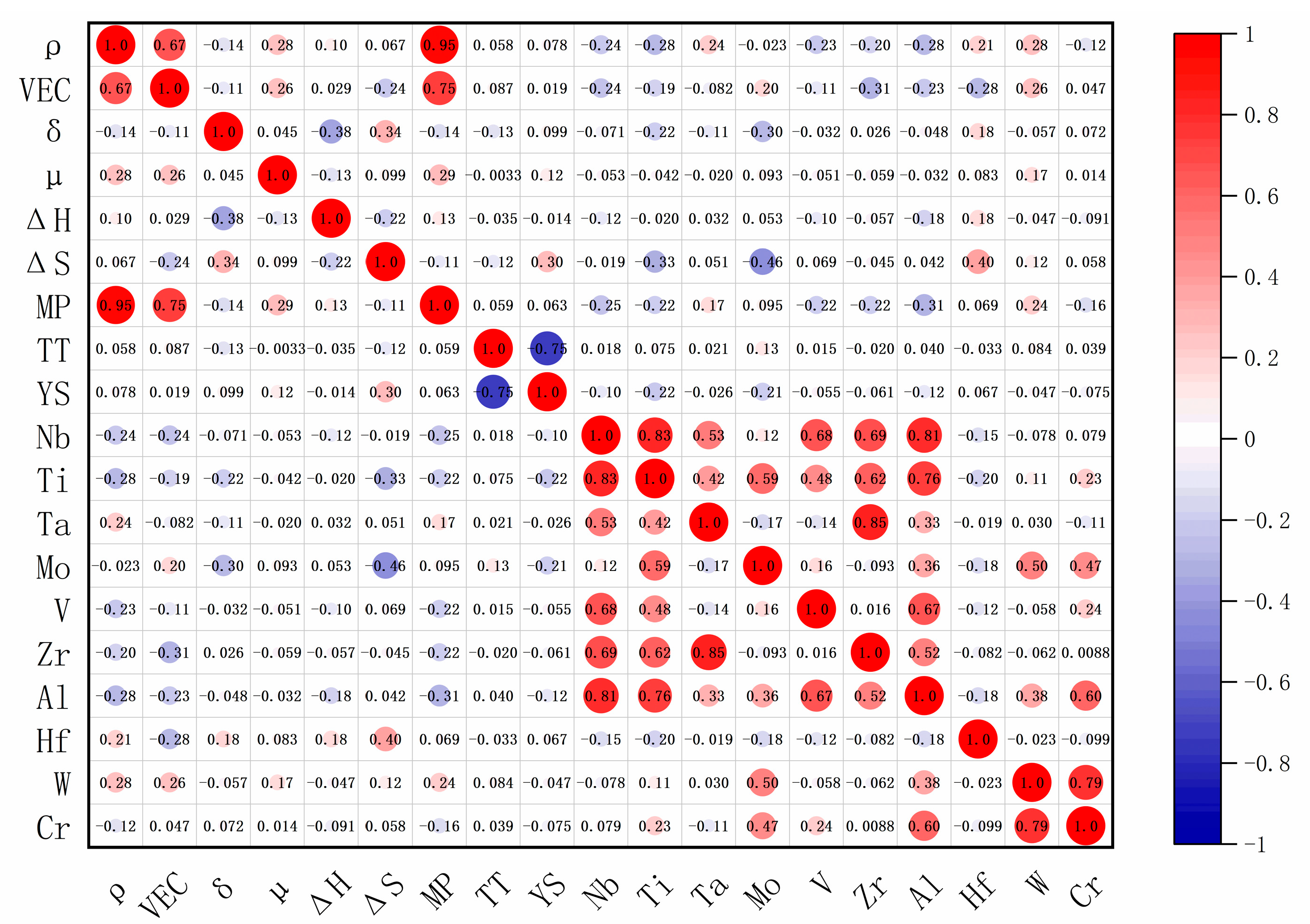
A total of 652 sets of high-entropy alloy data were collected and processed, and the composition, property, and performance dataset of refractory high-entropy alloy was established. The key parameters that affect the mechanical properties of the refractory high-entropy alloy, including atomic size difference (δ), test temperature (TT), mixing entropy (ΔS), titanium (Ti) and molybdenum (Mo), were determined by correlation analysis of the dataset.

(2)

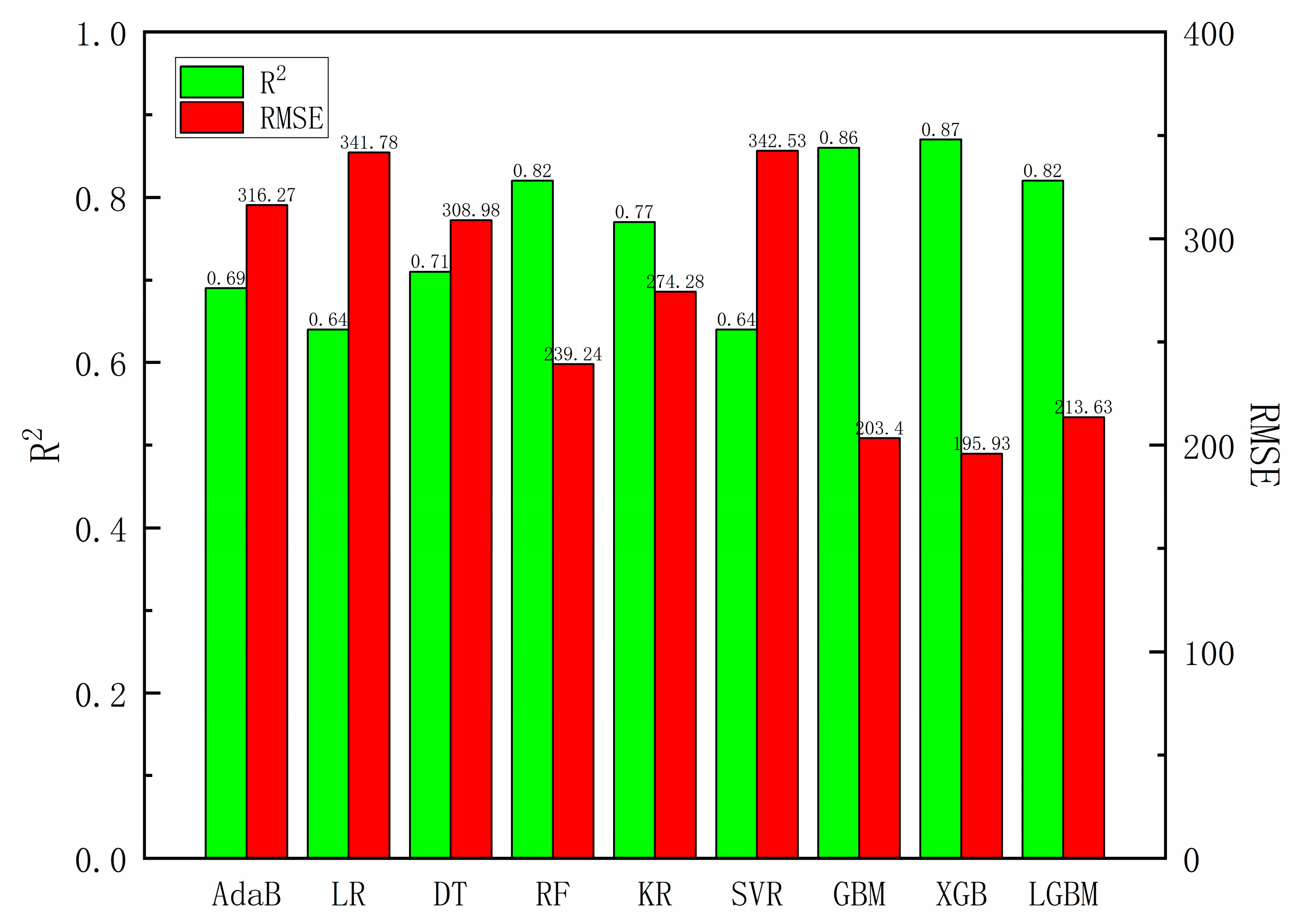
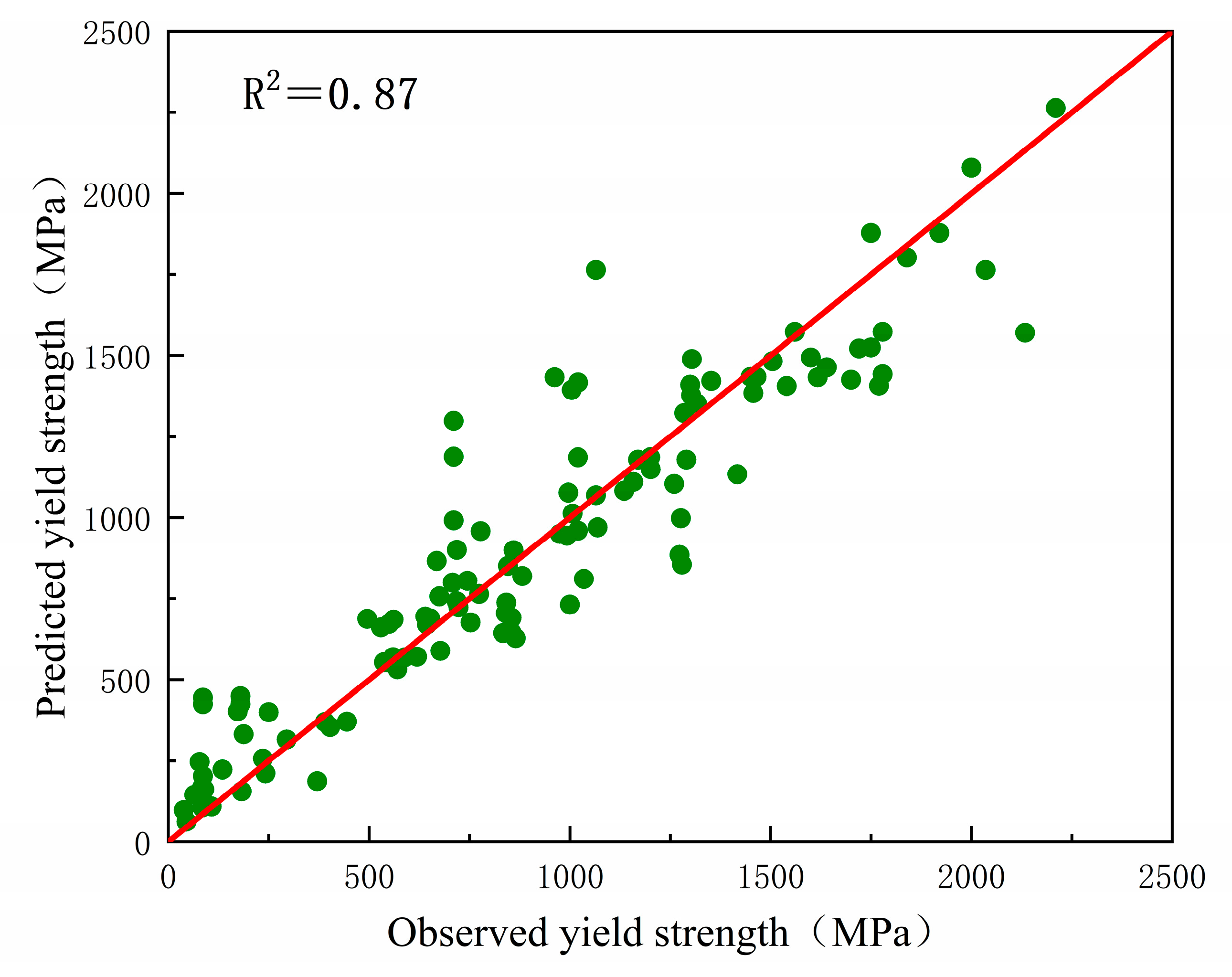
Based on the literature data, nine kinds of machine learning models were established, and the optimal hyperparameters were found by the combination of grid search and Bayesian optimization. The XGB model was selected as the prediction model for the mechanical properties of the high-entropy alloy, and the R2 and RMSE of the model reached 0.87 and 195.67 Mpa, respectively. The average prediction error of the XGB model was 12.62% through internal evaluation of randomly selected test set samples. By vacuum arc melting preparation, Ti27.5Zr26.5Nb25.5Ta8.5Al12 refractory high-entropy alloys were prepared for external data validation. The yield strength was 1365 MPa, the alloy experiment models predicted a yield strength of 1304.71 MPa, and the prediction model’s error was 3.8%. The results show that the model has a strong ability to predict the yield strength of the unknown high-entropy alloy.

(3)

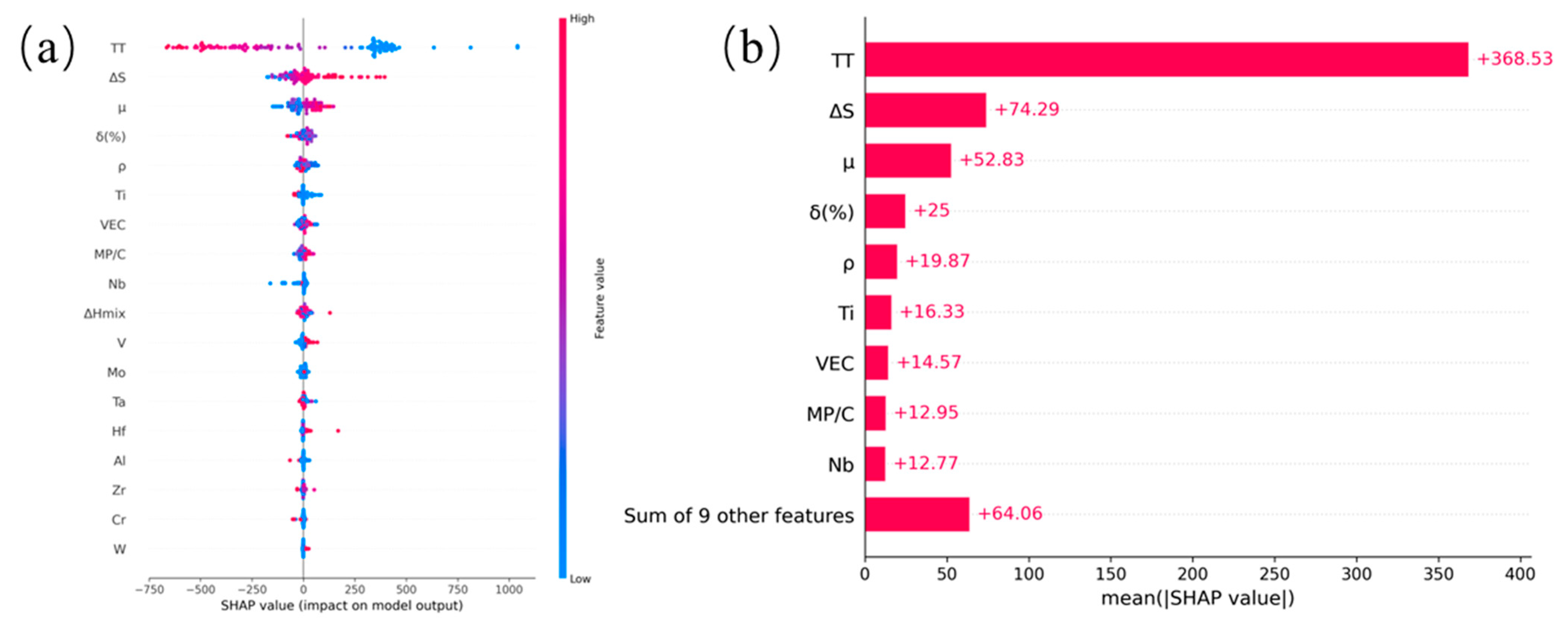
SHAP interpretable analysis of the model shows that the absolute values of TT, ΔS, and μ are 368.53, 74.29, and 52.83, respectively, which are significantly higher than other features. These results indicate that TT, ΔS, and μ have a great influence on the yield strength of refractory high-entropy alloys. In the subsequent material design, materials with desired properties can be synthesized by adjusting these three parameters.

References

1. Senkov, O.N.; Isheim, D.; Seidman, D.N.; Pilchak, A.L. Development of a Refractory High Entropy Superalloy. Entropy 2016, 18, 102. [Google Scholar] [CrossRef]
2. Tan, C.; Weng, F.; Sui, S.; Chew, Y.; Bi, G. Progress and perspectives in laser additive manufacturing of key aeroengine materials. Int. J. Mach. Tools Manuf. 2021, 170, 103804. [Google Scholar] [CrossRef]
3. Zhang, X.S.; Chen, Y.J.; Hu, J.L. Recent advances in the development of aerospace materials. Prog. Aerosp. Sci. 2018, 97, 22–34. [Google Scholar] [CrossRef]
4. Wang, Z.; Chen, S.; Yang, S.; Luo, Q.; Jin, Y.; Xie, W.; Zhang, L.; Li, Q. Light-weight refractory high-entropy alloys: A comprehensive review. J. Mater. Sci. Technol. 2023, 151, 41–65. [Google Scholar] [CrossRef]
5. Senkov, O.N.; Wilks, G.B.; Miracle, D.B.; Chuang, C.P.; Liaw, P.K. Refractory high-entropy alloys. Intermetallics 2010, 18, 1758–1765. [Google Scholar] [CrossRef]
6. Maiti, S.; Steurer, W. Structural-disorder and its effect on mechanical properties in single-phase TaNbHfZr high-entropy alloy. Acta Mater. 2016, 106, 87–97. [Google Scholar] [CrossRef]
7. Wang, M.L.; Lu, Y.P.; Lan, J.G.; Wang, T.M.; Zhang, C.; Cao, Z.Q.; Li, T.J.; Liaw, P.K. Lightweight, ultrastrong and high thermal-stable eutectic high-entropy alloys for elevated-temperature applications. Acta Mater. 2023, 248, 118806. [Google Scholar] [CrossRef]
8. Yao, H.W.; Qiao, J.W.; Hawk, J.A.; Zhou, H.F.; Chen, M.W.; Gao, M.C. Mechanical properties of refractory high-entropy alloys: Experiments and modeling. J. Alloys Compd. 2017, 696, 1139–1150. [Google Scholar] [CrossRef]
9. Li, T.; Chen, J.-X.; Liu, T.-W.; Chen, Y.; Luan, J.-H.; Jiao, Z.-B.; Liu, C.-T.; Dai, L.-H. D022 precipitates strengthened W-Ta-Fe-Ni refractory high-entropy alloy. J. Mater. Sci. Technol. 2024, 177, 85–95. [Google Scholar] [CrossRef]
10. Xiong, W.; Guo, A.X.Y.; Zhan, S.; Liu, C.T.; Cao, S.C. Refractory high-entropy alloys: A focused review of preparation methods and properties. J. Mater. Sci. Technol. 2023, 142, 196–215. [Google Scholar] [CrossRef]
11. Karantzalis, A.E.; Poulia, A.; Georgatis, E.; Petroglou, D. Phase formation criteria assessment on the microstructure of a new refractory high entropy alloy. Scr. Mater. 2017, 131, 51–54. [Google Scholar] [CrossRef]
12. Han, Z.D.; Chen, N.; Zhao, S.F.; Fan, L.W.; Yang, G.N.; Shao, Y.; Yao, K.F. Effect of Ti additions on mechanical properties of NbMoTaW and VNbMoTaW refractory high entropy alloys. Intermetallics 2017, 84, 153–157. [Google Scholar] [CrossRef]
13. Juan, C.C.; Tsai, M.H.; Tsai, C.W.; Lin, C.M.; Wang, W.R.; Yang, C.C.; Chen, S.K.; Lin, S.J.; Yeh, J.W. Enhanced mechanical properties of HfMoTaTiZr and HfMoNbTaTiZr refractory high-entropy alloys. Intermetallics 2015, 62, 76–83. [Google Scholar] [CrossRef]
14. Singh, P.; Vela, B.; Ouyang, G.; Argibay, N.; Cui, J.; Arroyave, R.; Johnson, D.D. A ductility metric for refractory-based multi-principal-element alloys. Acta Mater. 2023, 257, 119104. [Google Scholar] [CrossRef]
15. Guo, S.; Ng, C.; Lu, J.; Liu, C.T. Effect of valence electron concentration on stability of fcc or bcc phase in high entropy alloys. J. Appl. Phys. 2011, 109, 103505. [Google Scholar] [CrossRef]
16. Catal, A.A.; Bedir, E.; Yilmaz, R.; Swider, M.A.; Lee, C.; El-Atwani, O.; Maier, H.J.; Ozdemir, H.C.; Canadinc, D. Machine learning assisted design of novel refractory high entropy alloys with enhanced mechanical properties. Comput. Mater. Sci. 2024, 231, 112612. [Google Scholar] [CrossRef]
17. Yan, Y.G.; Lu, D.; Wang, K. Accelerated discovery of single-phase refractory high entropy alloys assisted by machine learning. Comput. Mater. Sci. 2021, 199, 110723. [Google Scholar] [CrossRef]
18. Wen, C.; Zhang, Y.; Wang, C.; Huang, H.; Wu, Y.; Lookman, T.; Su, Y. Machine-Learning-Assisted Compositional Design of Refractory High-Entropy Alloys with Optimal Strength and Ductility. Engineering 2024, 46, 214–223. [Google Scholar] [CrossRef]
19. Debnath, A.; Krajewski, A.M.; Sun, H.; Lin, S.; Ahn, M.; Li, W.J.; Priya, S.; Singh, J.; Shang, S.L.; Beese, A.M.; et al. Generative deep learning as a tool for inverse design of high entropy refractory alloys. J. Mater. Inform. 2021, 1, 3. [Google Scholar] [CrossRef]
20. Qu, N.; Zhang, Y.; Liu, Y.; Liao, M.Q.; Han, T.Y.; Yang, D.N.; Lai, Z.H.; Zhu, J.C.; Yu, L. Accelerating phase prediction of refractory high entropy alloys via machine learning. Phys. Scr. 2022, 97, 125710. [Google Scholar] [CrossRef]
21. Cheng, C.; Zou, Y. Accelerated discovery of nanostructured high-entropy alloys and multicomponent alloys via high-throughput strategies. Prog. Mater. Sci. 2025, 151, 101429. [Google Scholar] [CrossRef]
22. Churyumov, A.Y.; Kazakova, A.A. Prediction of True Stress at Hot Deformation of High Manganese Steel by Artificial Neural Network Modeling. Materials 2023, 16, 1083. [Google Scholar] [CrossRef] [PubMed]
23. Klimenko, D.; Stepanov, N.; Li, J.; Fang, Q.H.; Zherebtsov, S. Machine Learning-Based Strength Prediction for Refractory High-Entropy Alloys of the Al-Cr-Nb-Ti-V-Zr System. Materials 2021, 14, 7213. [Google Scholar] [CrossRef] [PubMed]
Figure 1. Correlation coefficient heat map.
Metals 15 00371 g001
Figure 2. R2 and RMSE for different machine learning models.
Metals 15 00371 g002
Figure 3. Relationship between real yield strength and predicted yield strength.
Metals 15 00371 g003
Figure 4. SHAP analysis results: (a) the influence of different SHAP characteristics on the predicted results of the model; (b) the importance of different features to the model’s predictions.
Metals 15 00371 g004