Analysis of Magneto-Piezoelastic Anisotropic Materials

Abstract

The paper is concerned with the analysis of magneto-piezoelastic anistropic materials. Analytical modeling of magneto-piezoelastic materials is essential for the design and applications in the smart composite structures incorporating them as actuating and sensing constituents. It is shown that Green’s function method is applicable to time harmonic magneto-elastic-piezoelectricity problems using the boundary integral technique, and the exact analytical solutions are obtained. As an application, a two-dimensional static plane-strain problem is considered to investigate the effect of magnetic field on piezoelectric materials. The closed-form analytical solutions are obtained for a number of boundary conditions for all components of the magneto-piezoelectric field. As a special case, numerical results are presented for two-dimensional static magneto-electroelastic field of a piezoelectric solid subjected to a concentrated line load and an electric charge. The numerical solutions are obtained for three different piezoelectric materials and they demonstrate a substantial dependence of the stress and electric field distribution on the constitutive properties and magnetic flux.

1. Introduction

The unique properties of magneto-piezoelastic materials render them suitable candidates for a broad range of novel practical applications in the form of components, devices and smart structures and systems; for example their sensitivity to external stimuli (electric and magnetic fields, temperature, etc.) can be exploited for frequency tunable devices such as resonators, phase shifters, delay lines and filters, as magnetic field sensors, energy harvesting transducers, miniature antennas, etc. (see [1,2,3,4,5,6]). Other attractive potential applications of some classes of magnetoelectric materials include data storage devices and spintronics [7], biomedical sensors for EEG/MEG and other relevant equipment [8,9].

Three-dimensional models for magnetoelectric composite materials are obtained in [10,11]. Two models are developed; one model uses dynamic force and thermal balance and the time-varying form of Maxwell’s equations to determine closed-form expressions for the effective properties and the second model uses the quasi-static approximation of the aforementioned constitutive equations.

Analysis of electromechanical coupling in soft dielectrics is carried out in [12]. It is shown that the required electric field to produce large deformations in electroactive soft elastomers can be significantly reduced. The finite element models are developed for the magnetoactive elastomers in [13]. In particular, it is demonstrated that the magneto-mechanical coupling of magnetoactive elastomers, when subjected to aligned loading conditions, depends not only on the magnetic susceptibility, but also, strongly, on its derivative with respect to the deformation.

The exact solution for simply supported magneto-electro-elastic laminated plates was obtained in [14]. The three-dimensional discrete-layer model is developed in [15] for the hygro-thermo-piezoelectric laminated plates under the coupled effects of mechanical, electrical, thermal and moisture fields. The hygro-thermo-magneto-electro-mechanical loading of laminated and functionally graded cylinders was investigated in [16]. The analytical solution for hygrothermal stresses in functionally graded piezoelectric material subjected to a constant magnetic field is obtained in [17].

In view of the aforementioned (and many more) practical applications, the main objective of this paper is to develop an accurate mechanical model that can be used to analyze and design magneto-piezoelastic smart structures.

Following this introduction, the basic relations describing magneto-piezoelastic materials are formulated in Section 2, and two magneto-elasto-piezoelectric states are considered in Section 3. The first state represents the solution of the magneto-elasto-piezoelectric problems with finite domains and general loading conditions. The second state represents the fundamental solution in the case of an infinite magneto-elasto-piezoelectric medium subjected to an impulsive point source and an impulsive point charge. The two-dimensional magneto-piezoelastic problem is analyzed in Section 4, and the solutions for problems with loads applied to the boundary are obtained in Section 5. The case of concentrated electric charge applied to magneto-piezoelastic solid with free boundary is solved in Section 6. Obtained results are discussed in Section 7, and finally Section 8 concludes the paper.

2. Basic Equations

Combined action of piezoelectricity, continuum mechanics and magnetism is open for discussion, although the mathematical development for possible applications is feasible for many engineering problems. As far as the mechanical modeling aspect is concerned, the further mathematically rigorous analysis is definetly required. The object of this study is to develop a rigorous mechanical model to describe the behavior and interrelations of physical phenomenon combining all these three fields.

In the direct piezoelectric effect, the application of an external mechanical loading induces an electrical response in the material. In the converse effect, an applied electrical field makes the material strained. The applied electromagnetic field induces currents in a solid, which in turn give rise to Lorentz body force J × B, where J is induced current, and B is magnetic flux. Lorentz force enters the magneto-piezoelastic equation of motion as an extrenal body force.

Electromagnetic and elastic fields in a piezoelectric medium are fully described by the equations of motion of a continuous medium

$${\mathrm{\sigma }}_{ij,j}+F_i=\text{ρ}{\ddot{u}}_i$$

(1)

combined with Maxwell’s equations

$$curl \hspace{0.17em}E\hspace{0.17em}\hspace{0.17em}=-\frac{\partial B}{\partial t},\hspace{1em}div \hspace{0.17em}D=q$$

(2)

$$curl \hspace{0.17em}H\hspace{0.17em}\hspace{0.17em}=\hspace{0.17em}\hspace{0.17em}\hspace{0.17em}J\hspace{0.17em}+\hspace{0.17em}\hspace{0.17em}\frac{\partial D}{\partial t},\hspace{1em}div \hspace{0.17em}B=0$$

(3)

and the constitutive equations

$$B={\text{μ}}_{e}H D=\mathrm{\epsilon }\hspace{0.17em}E$$

(4)

$$J\hspace{0.17em}\hspace{0.17em}=\hspace{0.17em}\hspace{0.17em}\hspace{0.17em}\mathrm{\gamma }(E\hspace{0.17em}+\hspace{0.17em}\hspace{0.17em}\frac{\partial u}{\partial t}\times B)$$

(5)

where q, μ_e, ε and γ are electric charge density, magnetic permeability, permittivity and conductivity, respectively.

The stresses σ_ij, electric displacement $D=\left\{D_i\right\}$ and magnetic flux B are related to the strains ${\mathrm{\epsilon }}_{ij}$ and the electric and magnetic fields $E=\left\{E_i\right\}$, $H=\left\{H_i\right\}$ through the constitutive equations.

Consider a homogeneous magneto-piezoelastic anisotropic solid $\mathrm{\Omega }$ with boundary $\mathrm{\Gamma }$ subjected to a uniform magnetic field H. The equations of motion are given by

$$\hspace{0.17em}div\hspace{0.17em}\mathrm{\sigma } +(J\times B)+f=\mathrm{\rho }\ddot{u}$$

(6)

where $\mathrm{\sigma }=\left\{{\mathrm{\sigma }}_{ij}\right\}$, $u=\left\{u_i\right\}$, $\mathrm{\rho }$, $f=\left\{f_i\right\}$, $i=\text{1,2,3}$, are stresses, elastic displacements, mass density and body force per unit volume, respectively.

The strains $\mathrm{\epsilon }=\left\{{\mathrm{\epsilon }}_{ij}\right\}$ and electric field $E=\left\{E_i\right\}$ are related to elastic displacements and electric potential $\mathrm{\phi }$ through the equations

$${\mathrm{\epsilon }}_{ij}=\frac{1}{2}(u_{i,j}+u_{j,i}),\hspace{1em}{E}_i=-\hspace{0.17em}\hspace{0.17em}{\text{φ}}_{,i}$$

(7)

The constitutive relations for linear piezoelasticity are, see, e.g., [18]:

$${\mathrm{\sigma }}_{ij}=c_{ijkl}{\mathrm{\epsilon }}_{kl}-e_{kij}{E}_k\hspace{1em}\hspace{1em}{D}_i=e_{ikl}{\mathrm{\epsilon }}_{kl}+{\mathrm{\epsilon }}_{ik}{E}_k$$

(8)

where $c_{ijkl}$, $e_{ijk}$, and ${\mathrm{\epsilon }}_{ij}$ are the elastic, piezoelectric and dielectric material constants, respectively, satisfying the following symmetry relations:

$$c_{jikl}=c_{ijlk}=c_{jikl}=c_{klij}\hspace{1em}\hspace{1em}{e}_{kij}=e_{kji}\hspace{1em}\hspace{1em}{\mathrm{\epsilon }}_{ik}={\mathrm{\epsilon }}_{ki}$$

(9)

The combination of Equations (6)–(9) results in a system of four partial differential equations coupling the displacement components and electric potential; namely

$$c_{ijkl}{u}_{k,lj}+e_{kij}{\text{φ}}_{,kj}+{(J\times B)}_i+f_i=\text{ρ}{\ddot{\mathrm{u}}}_i$$

(10)

$$e_{ikl}{u}_{k,li}-{\mathrm{\epsilon }}_{ik}{\text{φ}}_{,ki}=q$$

(11)

The admissible boundary conditions are

$$u_i=\overline{u_i}\hspace{1em} or \hspace{1em}\hspace{1em}{\mathrm{\sigma }}_{ij}{\text{η}}_j=\overline{{\text{τ}}_i}\hspace{1em}\hspace{1em}\text{φ}=\overline{\text{φ}}\hspace{1em} or \hspace{1em}{D}_i{\text{η}}_i=-\overline{q}$$

(12)

where $\overline{u_i},$ $\overline{{\text{τ}}_i},$ $\overline{\text{φ}},$ and $\overline{q}$ denote the specified values.

3. Representation Formulae

Consider two magneto-elasto-piezoelectric states, namely $(u,\text{σ, φ},D)$ and $(u^{\prime },{\mathrm{\sigma }}^{\prime },{\text{φ}}^{\prime },D^{\prime })$. The first state represents the solution of magneto-elasto-piezoelectric problems with finite domains and general loading conditions. The second state represents the fundamental solution of the case of an infinite magneto-elasto-piezoelectric medium subjected to an impulsive point source and an impulsive point charge. Each state is assumed to satisfy the following governing equations:

First State

$${\mathrm{\sigma }}_{ij,j}+{(J\times B)}_i+f_i=\text{ρ}{\ddot{\mathrm{u}}}_i\hspace{1em}\hspace{1em}{D}_{i,i}=q$$

(13)

$${\mathrm{\sigma }}_{ij}=c_{jikl}{u}_{k,l}+e_{kij}{\text{φ}}_{,k}\hspace{1em}\hspace{1em}{D}_i=e_{ikl}{u}_{k,l}-{\text{ε}}_{ik}{\text{φ}}_{,k}$$

(14)

Second State:

$${\mathrm{\sigma }}_{ij,j}^{\prime }+{(J^{\prime }\times B^{\prime })}_i+f_i^{\prime }=\text{ρ}{\ddot{\mathrm{u}}}_i^{\prime },\hspace{1em}{D}_{i,i}^{\prime }=q^{\prime }$$

(15)

Let a function ${\Pi }_{12}$ be the work done, given by the equation

$${\Pi }_{12}={\displaystyle {\int }_B}{F}_i\cdot u_i^{\prime }dv+{\displaystyle {\int }_{\Gamma }}{t}_i\cdot u_i^{\prime }dA-{\displaystyle {\int }_B}q\cdot {\text{φ}}^{\prime }dv+{\displaystyle {\int }_{\Gamma }}{D}_n\cdot {\text{φ}}^{\prime }dA$$

(16)

where the first two terms represent magneto-mechanical work, and the last two terms represent electric work. Here $D_n=D\cdot n$.

Similarly, let a second function ${\Pi }_{21}$ be the work done, given by the equation

$${\Pi }_{21}={\displaystyle {\int }_B}{F}_i^{\prime }\cdot u_{i}dv+{\displaystyle {\int }_{\Gamma }}{t}_i^{\prime }\cdot u_{i}dA-{\displaystyle {\int }_B}{q}^{\prime }\cdot \text{φ}dv+{\displaystyle {\int }_{\Gamma }}{D}_n^{\prime }\cdot \text{φ}dA$$

(17)

It can be shown that ${\Pi }_{12}={\Pi }_{21}$, see [19,20], where

$$F_i=(J\times B{)}_i+f_i\hspace{0.17em},\hspace{0.17em}\hspace{0.17em}\hspace{0.17em}{F}_i^{\prime }=(J^{\prime }\times B^{\prime }{)}_i+f_i^{\prime }$$

(18)

Representation of magneto-elasto-piezoelectricity is now based on two independent loading conditions for the second state, where a unit force and a unit charge are applied at a point $\mathrm{\xi }$ of the magneto-elasto-piezoelectric medium, known as the “source point.”

Case I: Let the body force and electric charge density for the second state be given by

$$F^{\prime }(x,t)=\mathrm{\delta }(x-\text{ξ}){\text{e}}_j\hspace{0.17em},\hspace{0.17em}\hspace{0.17em}\hspace{0.17em}\hspace{0.17em}{q}^{\prime }(x^{\prime },t)=0$$

(19)

where e is a unit vector along the x-axis, specifying the direction of the unit force, and

$$\text{δ}(x)=\text{δ}(x_1)\text{δ}(x_2)\text{δ}(x_3).\hspace{0.17em}\hspace{0.17em}\hspace{0.17em}\hspace{0.17em}\text{Also} \hspace{1em}{u}^{\prime }(x,t)=0,\hspace{1em}\text{φ}(x,t)=0,\hspace{1em} \text{if}\hspace{0.17em} \hspace{1em}t<0$$

(20)

We introduce the following notation for the applied loading given by Equation (19):

$$u_i^{\prime }(x,t)=U_{ij}(x,\text{ξ},t)\hspace{1em}{\text{φ}}^{\prime }(x,t)=U_{4j}(x,\text{ξ},t)$$

(21)

$$t_i^{\prime }(x,t)=T_{ji}(\text{ξ},x,t),\hspace{1em}{D}_n^{\prime }(x,t)=T_{j4}(\text{ξ},x,t)$$

(22)

where U_ij and U_4j are Green’s functions representing the displacement (in the i-direction) and the electric potential, respectively, at the field point x due to a unit force applied at ξ in the j-direction. T_ji and T_j4 (derivatives of Green’s functions) represent the traction on the boundary (in the i-direction) and the normal component of the electric displacement, respectively, at x when the unit force is applied at ξ.

Case II: Let the body force and electric charge density for the second state be given by

$$F^{\prime }(x,t),\hspace{1em}{q}^{\prime }(x,t)=-\text{δ}(x-\text{ξ})\text{δ}(t)$$

(23)

Introduce

$$u_i^{\prime }(x,t)=U_{i4}(x,\text{ξ},t),\hspace{1em}\hspace{1em}{\text{φ}}^{\prime }(x,t)=U_{44}(x,\text{ξ},t)$$

(24)

$$t_i^{\prime }(x,t)=T_{4i}(\text{ξ},x,t),\hspace{1em}\hspace{1em}{D}_n^{\prime }(x,t)=T_{44}(\text{ξ},x,t)$$

(25)

where the variables have the same meaning as described previously with the exception a negative unit charge is applied at the source point.

As ${\Pi }_{12}={\Pi }_{21}$ for the Case I:

$${\displaystyle {\int }_B}{F}_i\cdot u_i^{\prime }dv+{\displaystyle {\int }_{\Gamma }}{t}_i\cdot u_i^{\prime }dA-{\displaystyle {\int }_B}q\cdot {\text{φ}}^{\prime }dv+{\displaystyle {\int }_{\Gamma }}{D}_n\cdot {\text{φ}}^{\prime }dA=\hspace{0.17em}\hspace{0.17em}{\displaystyle {\int }_B}{F}_i^{\prime }\cdot u_{i}dv+{\displaystyle {\int }_{\Gamma }}{t}_i^{\prime }\cdot u_{i}dA-{\displaystyle {\int }_B}{q}^{\prime }\cdot \text{φ}dv+{\displaystyle {\int }_{\Gamma }}{D}_n^{\prime }\cdot \text{φ}dA$$

(26)

or

$$\begin{array}{c}{\displaystyle {\int }_B}{U}_{ij}(x,\text{ξ},t)\cdot F_i(x,t)dv+{\displaystyle {\int }_{\Gamma }}{U}_{ij}(x,\text{ξ},t)\cdot t_i(x,t)dA\hspace{0.17em}-{\displaystyle {\int }_B}{U}_{4j}(x,\text{ξ},t)\cdot qdv+{\displaystyle {\int }_{\Gamma }}{U}_{4j}(x,\text{ξ},t)\cdot D_{n}dA=\\ {\displaystyle {\int }_V}\text{δ}(x-\text{ξ})\text{δ}(t)e_j\cdot u_{i}dv+{\displaystyle {\int }_{\Gamma }}{T}_{ji}(\text{ξ},x,t)\cdot u_i(x,t)dA+{\displaystyle {\int }_{\Gamma }}{T}_{i4}(\text{ξ},x,t)\cdot \text{φ}dA\end{array}$$

(27)

Integrating with respect to t yields

$$\begin{array}{c}{u}_j(\text{ξ},t)={\displaystyle {\int }_{\Gamma }}{\displaystyle {\int }_0^t}[U_{ij}(x,\text{ξ},t-\text{τ})t_i(x,\text{τ}) +U_{4j}(x,\text{ξ},t-\mathrm{\tau })D_n(x,\text{τ})]d\text{τ}dA\hspace{0.17em}-\\ {\displaystyle {\int }_{\Gamma }}{\displaystyle {\int }_0^t}[T_{ji}(x,\text{ξ},t-\text{τ})u_i(x,\text{τ}) +T_{j4}(x,\text{ξ},t-\text{τ})\text{φ}(x,\text{τ})]d\text{τ}dA\hspace{0.17em}+\\ {\displaystyle {\int }_B}{\displaystyle {\int }_0^t}[U_{ij}(x,\text{ξ},t-\mathrm{\tau })F_i(x,\text{τ}) -U_{4j}(x,\text{ξ},t-\text{τ})q(x,\text{τ})]d\text{τ}dv\end{array}$$

(28)

Similarly, for Case II:

$$\begin{array}{c}{\displaystyle {\int }_B}{F}_i\cdot u_i^{\prime }dv+{\displaystyle {\int }_{\Gamma }}{t}_i\cdot u_i^{\prime }dA-{\displaystyle {\int }_B}q\cdot {\text{φ}}^{\prime }dv+{\displaystyle {\int }_{\Gamma }}{D}_n\cdot {\text{φ}}^{\prime }dA=\\ {\displaystyle {\int }_B}{F}_i^{\prime }\cdot u_{i}dv+{\displaystyle {\int }_{\Gamma }}{t}_i^{\prime }\cdot u_{i}dA-{\displaystyle {\int }_B}{q}^{\prime }\cdot \text{φ}dv+{\displaystyle {\int }_{\Gamma }}{D}_n^{\prime }\cdot \text{φ}dA\end{array}$$

(29)

$$\begin{array}{c}{\displaystyle {\int }_B}{F}_i\cdot U_{i4}(x,\text{ξ},t)dv+{\displaystyle {\int }_{\Gamma }}{t}_i\cdot U_{i4}(x,\text{ξ},t)dA-{\displaystyle {\int }_B}q\cdot U_{44}(x,\text{ξ},t)dv+\\ {\displaystyle {\int }_{\Gamma }}{D}_n\cdot U_{44}(x,\text{ξ},t)dA={\displaystyle {\int }_{\Gamma }}{T}_{4i}(\text{ξ},x,t)\cdot u_{i}dA+{\displaystyle {\int }_B}\text{δ}(x-\text{ξ})\text{δ}(t)\cdot \text{φ}dv+{\displaystyle {\int }_{\Gamma }}{T}_{44}(\text{ξ},x,t)\cdot \text{φ}(x,t)dA\end{array}$$

(30)

Integrating with respect to t yields

$$\begin{array}{c}\text{φ}(\text{ξ},t)={\displaystyle {\int }_{\Gamma }}{\displaystyle {\int }_0^t}[U_{i4}(x,\text{ξ},t-\text{τ})t_i(x,\text{τ})+U_{44}(\text{ξ},x,t-\text{τ})\cdot D_n(\text{ξ},\mathrm{\tau })]d\text{τ}dA\hspace{0.17em}\hspace{0.17em}-\\ {\displaystyle {\int }_{\Gamma }}{\displaystyle {\int }_0^t}[T_{4i}(\text{ξ},x,t-\text{τ})u_i(x,\text{τ})+T_{44}(\text{ξ},x,t-\text{τ})\text{φ}(x,\text{τ})]d\text{τ}dA\hspace{0.17em}\hspace{0.17em}+\\ {\displaystyle {\int }_B}{\displaystyle {\int }_0^t}[U_{i4}(x,\text{ξ},t-\text{τ})F_i(x,\text{τ})-U_{44}(x,\text{ξ},t-\text{τ})q(x,\text{τ})]d\text{τ}dA\end{array}$$

(31)

4. Two-Dimensional Magneto-Piezoelastic Problem

The constitutive relations for the plane-strain case when ${\mathrm{\epsilon }}_{yy}$, ${\mathrm{\epsilon }}_{xy}$, ${\mathrm{\epsilon }}_{zy}=0$ is

$$\begin{array}{c}{\mathrm{\sigma }}_{xx}=c_{11}{\mathrm{\epsilon }}_{xx}+c_{13}{\mathrm{\epsilon }}_{zz}-e_{31}{E}_z,\hspace{1em}{\mathrm{\sigma }}_{zz}=c_{13}{\mathrm{\epsilon }}_{xx}+c_{33}{\mathrm{\epsilon }}_{zz}-e_{33}{E}_z\\ {\mathrm{\sigma }}_{xz}=2c_{44}{\mathrm{\epsilon }}_{xz}-e_{15}{E}_x,\hspace{1em}{D}_x=2e_{15}{\mathrm{\epsilon }}_{xz}+{\mathrm{\epsilon }}_{11}{E}_x\\ D_z=e_{31}{\mathrm{\epsilon }}_{xx}+e_{33}{\mathrm{\epsilon }}_{zz}+{\mathrm{\epsilon }}_{33}{E}_z\end{array}$$

(32)

The constitutive equations for the plane-stress case when ${\mathrm{\sigma }}_{yy}$, ${\mathrm{\sigma }}_{xy}$, ${\mathrm{\sigma }}_{yz}=0$ are obtained from the above equations by replacing $c_{11},c_{13},c_{33},e_{31},e_{33}$ and ${\mathrm{\epsilon }}_{33}$ by $(c_{11}-c_{12}^2/c_{11})$, $(c_{13}-c_{13}{c}_{12}/c_{11})$, $(c_{33}-c_{13}^2/c_{11})$, $(e_{31}-c_{12}{e}_{31}/c_{11})$, $(e_{33}-c_{13}{e}_{31}/c_{11})$, and $({\mathrm{\epsilon }}_{33}+e_{31}^2/c_{11})$, respectively. Here, $c_{11},c_{13},c_{33},c_{44}$ are elastic modulii; $e_{31},e_{33}$ and $e_{15}$ are piezoelectric constants; ${\mathrm{\epsilon }}_{11},{\mathrm{\epsilon }}_{33}$ are dielectric permittivities.

The equations of motion are

$$\begin{array}{c}\frac{\partial {\mathrm{\sigma }}_{xx}}{\partial x}+\frac{\partial {\mathrm{\sigma }}_{xz}}{\partial z}+f_x+{(J\times B)}_x=\mathrm{\rho }\frac{{\partial }^2{u}_x}{\partial t^2}\\ \frac{\partial {\mathrm{\sigma }}_{xz}}{\partial x}+\frac{\partial {\mathrm{\sigma }}_{zz}}{\partial z}+f_z+{(J\times B)}_z=\text{ρ}\frac{{\partial }^2{u}_z}{\partial t^2}\\ \frac{\partial D_x}{\partial x}+\frac{\partial D_z}{\partial z}=q\end{array}$$

(33)

Also

$$E_z=-\frac{\partial \text{φ}}{\partial x}\hspace{1em}\hspace{1em}{E}_z=-\frac{\partial \text{φ}}{\partial z}\hspace{1em}\hspace{1em}{\mathrm{\epsilon }}_{xx}=\frac{\partial u_x}{\partial x}\hspace{1em}\hspace{1em}{\mathrm{\epsilon }}_{zz}=\frac{\partial u_z}{\partial z} {\mathrm{\epsilon }}_{xz}=\frac{1}{2}\left(\frac{\partial u_x}{\partial z}+\frac{\partial u_z}{\partial x}\right)$$

(34)

Assume $H=\left\{H_1,0,0\right\}$, and substitute Equation (34) into the Equation (33), then

$$\begin{array}{c}{c}_{11}\frac{{\partial }^2{u}_x}{\partial x^2}+c_{44}\frac{{\partial }^2{u}_x}{\partial z^2}+(c_{13}+c_{44})\frac{{\partial }^2{u}_z}{\partial x\partial z}+(e_{31}+e_{15})\frac{{\partial }^2\text{φ}}{\partial x\partial z} +f_x=\text{ρ}\frac{{\partial }^2{u}_x}{\partial t^2}\\ c_{44}\frac{{\partial }^2{u}_z}{\partial x^2}+c_{33}\frac{{\partial }^2{u}_z}{\partial z^2}+(c_{13}+c_{44})\frac{{\partial }^2{u}_x}{\partial x\partial z}+e_{15}\frac{{\partial }^2\text{φ}}{\partial x^2} +e_{33}\frac{{\partial }^2\text{φ}}{\partial z^2}+{\text{μ}}_e{H}_1^2{\nabla }^2{u}_z+f_z=\mathrm{\rho }\frac{{\partial }^2{u}_z}{\partial t^2}\\ e_{15}\frac{{\partial }^2{u}_z}{\partial x^2}+e_{33}\frac{{\partial }^2{u}_z}{\partial z^2}+(e_{31}+e_{15})\frac{{\partial }^2{u}_x}{\partial x\partial z} -{\mathrm{\epsilon }}_{11}\frac{{\partial }^2\text{φ}}{\partial x^2}-{\mathrm{\epsilon }}_{33}\frac{{\partial }^2\text{φ}}{\partial z^2}=q\end{array}$$

(35)

Assume the general solution of the homogeneous equation with

$$\begin{array}{c}{f}_x=f_z=q=0,\hspace{1em}\frac{{\partial }^2{u}_x}{\partial t^2}=\frac{{\partial }^2{u}_z}{\partial t^2}=0\\ u_x=\frac{1}{2\mathrm{\pi }}{\displaystyle {\int }_{-\mathrm{\infty }}^{\mathrm{\infty }}}i\text{ξ}\left(A_1{e}^{-\text{α}|\text{ξ}|z}-A_2{e}^{\text{α}|\text{ξ}|z}\right)\hspace{0.17em}\hspace{0.17em}{e}^{-i\text{ξ}x}d\text{ξ}\\ u_z=\frac{1}{2\mathrm{\pi }}{\displaystyle {\int }_{-\mathrm{\infty }}^{\mathrm{\infty }}}|\text{ξ}|\left(B_1{e}^{-\text{α}|\text{ξ}|z}+B_2{e}^{\text{α}|\text{ξ}|z}\right)\hspace{0.17em}\hspace{0.17em}{e}^{-i\text{ξ}x}d\text{ξ}\\ \mathrm{\phi }=\frac{1}{2\mathrm{\pi }}{\displaystyle {\int }_{-\mathrm{\infty }}^{\mathrm{\infty }}}|\text{ξ}|\left(C_1{e}^{-\text{α}|\text{ξ}|z}+C_2{e}^{\text{α}|\text{ξ}|z}\right)\hspace{0.17em}\hspace{0.17em}{e}^{-i\text{ξ}x}d\text{ξ}\end{array}$$

(36)

The substitution of Equation (36) into Equation (35) yields

$$[P]{\langle A_1{B}_1{C}_1\rangle }^T=\left\{0\right\}\hspace{1em}\hspace{1em}[P]{\langle A_2{B}_2{C}_2\rangle }^T=\left\{0\right\}$$

(37)

where

$$[P]=\left(\begin{array}{ccc}{c}_{11}-c_{44}{\text{α}}^2& -(c_{13}+c_{44})\text{α}& -(e_{31}+e_{15})\text{α}\\ -(c_{13}+c_{44})\text{α}& (c_{33}{\text{α}}^2-c_{44})+{\text{μ}}_e{H}_1^2({\text{α}}^2-1)& e_{33}{\text{α}}^2-e_{15}\\ -(e_{31}+e_{15})\text{α}& e_{33}{\text{α}}^2-e_{15}& {\mathrm{\epsilon }}_{11}-{\mathrm{\epsilon }}_{33}{\text{α}}^2\end{array}\right)$$

(38)

and $\mathrm{\alpha }$ is the root of the characteristic equation

$$det [P]=0,\hspace{1em} or \hspace{1em}{\text{α}}^6+d_1{\text{α}}^4+d_2{\text{α}}^2+d_3=0$$

(39)

where $d_1,d_2$ and $d_3$ are real constants which depend on the magneto-piezoelastic properties of a material. Since $d_1,d_2$ and $d_3$ are real, the bi-quartic Equation (39) has three pairs of roots $(\pm {\text{α}}_1,\pm {\text{α}}_2,\pm {\text{α}}_3)$, where ${\mathrm{\alpha }}_1$ is a positive real number and ${\text{α}}_2$, ${\text{α}}_3$ are either positive real numbers or a pair of complex conjugates with positive real parts (${\text{α}}_3={\overline{\text{α}}}_2$ , where ${\overline{\text{α}}}_2$ denotes the complex conjugate of ${\text{α}}_2$).

Let us take the Fourier transform of the Equation (35) with respect to x, then

$$\begin{array}{c}(c_{44}\frac{d^2}{d{z}^2}-c_{11}{\text{ξ}}^2){\overline{u}}_x+(c_{13}+c_{44})i\text{ξ}\frac{d{\overline{u}}_z}{dz}+(e_{31}+e_{15})i\text{ξ}\frac{d\overline{\text{φ}}}{dz}=0\\ (c_{13}+c_{44})i\text{ξ}\frac{d{\overline{u}}_x}{dz}+\{(c_{33}\frac{d^2}{d{z}^2}-c_{44}{\text{ξ}}^2)+{\text{μ}}_e{H}_1^2(\frac{d^2}{d{z}^2}-{\text{ξ}}^2)\}{\overline{u}}_z +(e_{33}\frac{d^2}{d{z}^2}-e_{15}{\text{ξ}}^2)\overline{\text{φ}}=0\\ (e_{31}+e_{15})i\text{ξ}\frac{d{\overline{u}}_x}{dz}+(e_{33}\frac{d^2}{d{z}^2}-e_{15}{\text{ξ}}^2){\overline{u}}_z+(-{\mathrm{\epsilon }}_{33}\frac{d^2}{d{z}^2} +{\mathrm{\epsilon }}_{11}{\text{ξ}}^2)\overline{\text{φ}}=0\end{array}$$

(40)

The general solutions for Fourier transforms of displacements and elastic and electric potential are

$$\begin{array}{c}{\overline{u}}_x(\text{ξ},z)=i\text{ξ}{\displaystyle \sum _{j=1}^3}{\text{β}}_j\left(G_j{e}^{-{\text{α}}_j|\text{ξ}|z}-H_j{e}^{{\text{α}}_j|\text{ξ}|z}\right)\\ {\overline{u}}_z(\text{ξ},z)=|\text{ξ}|{\displaystyle \sum _{j=1}^3}{n}_j\left(G_j{e}^{-{\text{α}}_j|\text{ξ}|z}+H_j{e}^{{\text{α}}_j|\text{ξ}|z}\right)\\ \overline{\text{φ}}(\text{ξ},z)=|\text{ξ}|{\displaystyle \sum _{j=1}^3}{\text{δ}}_j\left(G_j{e}^{-{\text{α}}_j|\text{ξ}|z}+H_j{e}^{{\text{α}}_j|\text{ξ}|z}\right)\end{array}$$

(41)

where

$$\begin{array}{c}{\text{β}}_j=(c_{13}+c_{44})(e_{33}{{\text{α}}_j}^2-e_{15}){\text{α}}_j-\{(c_{33}{{\text{α}}_j}^2-c_{44}) +{\text{μ}}_e{H}_1^2({\text{α}}_j^2-1)\}(e_{31}+e_{15}){\text{α}}_j\\ {\text{η}}_j=(c_{11}-c_{44}{\text{α}}_j^2)(e_{33}{\text{α}}_j^2-e_{15})-(c_{13}+c_{44})(e_{31}+e_{15}){\text{α}}_j^2\\ {\text{δ}}_j=-(c_{44}{\text{α}}_j^2-c_{11})\{(c_{44}-c_{33}{\text{α}}_j^2)-{\text{μ}}_e{H}_1^2({\text{α}}_j^2-1)\} +{(c_{13}+c_{44})}^2{\text{α}}_j^2\end{array}$$

(42)

and $G_j(\text{ξ})$ and $H_j(\text{ξ})\hspace{0.17em},\hspace{0.17em}\hspace{0.17em}(j=\text{1,2,3})$ are obtained from the appropriate boundary and continuity conditions.

The stresses and electric potential in transform space are shown below

$$\begin{array}{c}{\overline{\mathrm{\sigma }}}_{zz}={\displaystyle \sum _{j=1}^3}{\text{ξ}}^2{d}_{2j}\left(G_j{e}^{-{\text{α}}_j|\text{ξ}|z}-H_j{e}^{{\text{α}}_j|\text{ξ}|z}\right), {\overline{\mathrm{\sigma }}}_{xx}={\displaystyle \sum _{j=1}^3}{\text{ξ}}^2{d}_{1j}\left(G_j{e}^{-{\text{α}}_j|\text{ξ}|z}-H_j{e}^{{\text{α}}_j|\text{ξ}|z}\right)\\ {\overline{\mathrm{\sigma }}}_{zz}={\displaystyle \sum _{j=1}^3}i\text{ξ}|\text{ξ}|d_{3j}\left(G_j{e}^{-{\text{α}}_j|\text{ξ}|z}+H_j{e}^{{\text{α}}_j|\text{ξ}|z}\right)\\ {\overline{D}}_x={\displaystyle \sum _{j=1}^3}i\text{ξ}|\text{ξ}|d_{4j}\left(G_j{e}^{-{\text{α}}_j|\text{ξ}|z}+H_j{e}^{{\text{α}}_j|\text{ξ}|z}\right), {\overline{D}}_z={\displaystyle \sum _{j=1}^3}{\text{ξ}}^2{d}_{5j}\left(G_j{e}^{-{\text{α}}_j|\text{ξ}|z}-H_j{e}^{{\text{α}}_j|\text{ξ}|z}\right)\end{array}$$

(43)

where

$$d_{1j}=c_{11}{\mathrm{\beta }}_j-c_{13}{\mathrm{\alpha }}_j{\mathrm{\eta }}_j-e_{31}{\mathrm{\alpha }}_j{\mathrm{\delta }}_j\hspace{1em}{d}_{2j}=c_{13}{\mathrm{\beta }}_j-c_{33}{\mathrm{\alpha }}_j{\mathrm{\eta }}_j-e_{33}{\mathrm{\alpha }}_j{\mathrm{\delta }}_j$$

(44)

$$d_{3j}=-c_{44}{\mathrm{\alpha }}_j{\mathrm{\beta }}_j-c_{44}{\mathrm{\eta }}_j-e_{15}{\mathrm{\delta }}_j\hspace{1em}{d}_{4j}=-e_{15}{\mathrm{\alpha }}_j{\mathrm{\beta }}_j-e_{15}{\mathrm{\eta }}_j+{\mathrm{\epsilon }}_{11}{\mathrm{\delta }}_j$$

(45)

$$d_{5j}=e_{31}{\mathrm{\beta }}_j-e_{33}{\mathrm{\alpha }}_j{\mathrm{\eta }}_j+{\mathrm{\epsilon }}_{33}{\mathrm{\alpha }}_j{\mathrm{\delta }}_j$$

(46)

The solutions for plane-stress problems are obtained by using the appropriate material parameters as explained above.

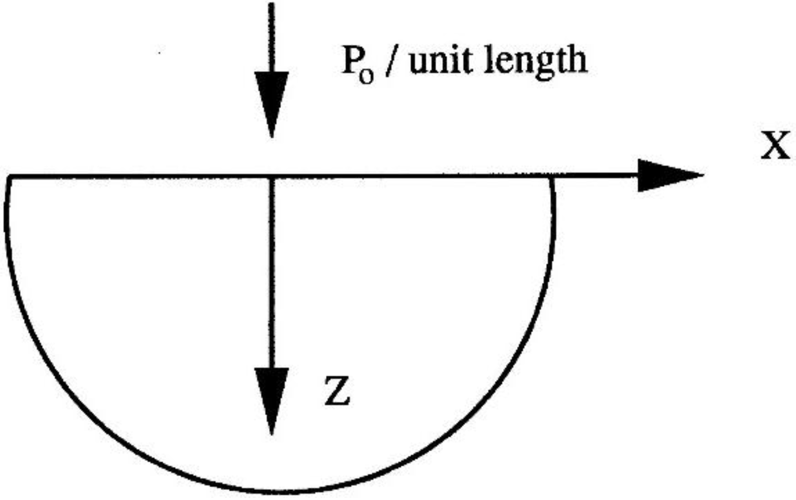
5. Solutions for Loads Applied to the Boundary

Assume a magneto-piezoelastic medium subjected to vertical line load and electric charge at the surface, see Figure 1.

Figure 1. Concentrated line load applicable to magneto-piezoelastic medium with free boundary.

Figure 1. Concentrated line load applicable to magneto-piezoelastic medium with free boundary.

The consideration of regularity conditions of field variables as $z\to \mathrm{\infty }$ implies that $H_j=0$. In the first case of a verical load of magnitude $P_0$ per unit length applied to the surface, the boundary conditions are

$${\mathrm{\sigma }}_{xz}(x,0)=0\hspace{1em}{\mathrm{\sigma }}_{zz}(x,0)=-P_0\mathrm{\delta }(x)\hspace{1em}{D}_z(x,0)=0$$

(47)

$${\overline{\mathrm{\sigma }}}_{zz}(x,0)=-P_0\hspace{1em}{\overline{\mathrm{\sigma }}}_{xz}(x,0)=0\hspace{1em}{\overline{D}}_z(x,0)=0$$

(48)

$${\mathrm{\xi }}^2{d}_{21}{G}_1+{\mathrm{\xi }}^2{d}_{22}{G}_2+{\mathrm{\xi }}^2{d}_{23}{G}_3=-P_0$$

(49)

$$d_{31}{G}_1+d_{32}{G}_2+d_{33}{G}_3=0\hspace{1em}{d}_{51}{G}_1+d_{52}{G}_2+d_{53}{G}_3=0$$

(50)

Solving

$$G_1=\frac{a_1}{{\mathrm{\xi }}^2},\hspace{1em}{G}_2=\frac{a_2}{{\mathrm{\xi }}^2},\hspace{1em}{G}_3=\frac{a_3}{{\mathrm{\xi }}^2}$$

(51)

Here

$$a_1=-\frac{(d_{32}{d}_{53}-d_{33}{d}_{52})P_0}{\Delta },\hspace{1em}{a}_2=-\frac{(d_{33}{d}_{51}-d_{31}{d}_{53})P_0}{\Delta }$$

(52)

$$a_3=-\frac{(d_{31}{d}_{52}-d_{32}{d}_{51})P_0}{\Delta }$$

(53)

$$\Delta =d_{31}(d_{52}{d}_{23}-d_{53}{d}_{22})-d_{32}(d_{51}{d}_{23}-d_{53}{d}_{21}) +d_{33}(d_{51}{d}_{22}-d_{52}{d}_{21})$$

(54)

$${\overline{u}}_x(\mathrm{\xi },z)=i\mathrm{\xi }\left({\mathrm{\beta }}_1{G}_1{e}^{-{\mathrm{\alpha }}_1|\mathrm{\xi }|z}+{\mathrm{\beta }}_2{G}_2{e}^{-{\mathrm{\alpha }}_2|\mathrm{\xi }|z}+{\mathrm{\beta }}_3{G}_3{e}^{-{\mathrm{\alpha }}_3|\mathrm{\xi }|z}\right)$$

(55)

$${\overline{u}}_z(\mathrm{\xi },z)=|\mathrm{\xi }|\left({\mathrm{\eta }}_1{G}_1{e}^{-\mathrm{\alpha }|\mathrm{\xi }|z}+{\mathrm{\eta }}_2{G}_2{e}^{-{\mathrm{\alpha }}_2|\mathrm{\xi }|z}+{\mathrm{\eta }}_3{G}_3{e}^{-{\mathrm{\alpha }}_3|\mathrm{\xi }|z}\right)$$

(56)

$$\overline{\mathrm{\phi }}(\mathrm{\xi },z)=|\mathrm{\xi }|\left({\mathrm{\delta }}_1{G}_1{e}^{-\mathrm{\alpha }|\mathrm{\xi }|z}+{\mathrm{\delta }}_2{G}_2{e}^{-\mathrm{\alpha }|\mathrm{\xi }|z}+{\mathrm{\delta }}_3{G}_3{e}^{-{\mathrm{\alpha }}_3|\mathrm{\xi }|z}\right)$$

(57)

$$u_x(x,z)= Real\hspace{0.17em}part\hspace{0.17em}of \hspace{1em}\frac{1}{\mathrm{\pi }}{\displaystyle {\int }_0^{\mathrm{\infty }}}i\mathrm{\xi }(\frac{{\mathrm{\beta }}_1{a}_1}{{\mathrm{\xi }}^2}{e}^{-\mathrm{\alpha }|\mathrm{\xi }|z}+\frac{{\mathrm{\beta }}_2{a}_2}{{\mathrm{\xi }}^2}{e}^{-{\mathrm{\alpha }}_2|\mathrm{\xi }|z} +\frac{{\mathrm{\beta }}_3{a}_3}{{\mathrm{\xi }}^2}{e}^{-{\mathrm{\alpha }}_3|\mathrm{\xi }|z})e^{i\mathrm{\xi }x}d\mathrm{\xi }$$

(58)

where

$$e^{i\mathrm{\xi }x}=\cos (\mathrm{\xi }x)+i\sin (\mathrm{\xi }x)\hspace{1em}{u}_x(x,z)=-{\displaystyle \sum _{j=1}^3}{\mathrm{\beta }}_j{a}_j{S}_j(x,z)$$

(59)

$${\mathrm{\alpha }}_2=k-il,\hspace{1em}{\mathrm{\alpha }}_3=k+il;\hspace{1em}(k,l>0)$$

(60)

$$u_x(x,z)=-{\displaystyle \sum _{j=1}^3}{\mathrm{\beta }}_j{a}_j{S}_j(x,z)$$

(61)

Here

$$S_1(x,z)=\frac{1}{\mathrm{\pi }}\arctan \left(\frac{x}{{\mathrm{\alpha }}_{1}z}\right)\hspace{1em}{S}_2=\frac{N-iT}{\mathrm{\pi }},\hspace{1em}{S}_3={\tilde{S}}_2$$

(62)

$$N=\frac{1}{2}\arctan \left(\frac{2kzx}{(l^2{z}^2+k^2{z}^2-x^2)}\right)\hspace{1em}T=\frac{1}{4}\ln \left(\frac{k^2{z}^2+{(lz+x)}^2}{(k^2{z}^2+{(lz-x)}^2}\right)$$

(63)

$${\overline{u}}_z(\mathrm{\xi },z)=|\mathrm{\xi }|\left({\mathrm{\eta }}_1\frac{a_1}{{\mathrm{\xi }}^2}{e}^{-{\mathrm{\alpha }}_1|\mathrm{\xi }|z}+{\mathrm{\eta }}_2\frac{a_2}{{\mathrm{\xi }}^2}{e}^{-{\mathrm{\alpha }}_2|\mathrm{\xi }|z}+{\mathrm{\eta }}_3\frac{a_3}{{\mathrm{\xi }}^2}{e}^{-{\mathrm{\alpha }}_3|\mathrm{\xi }|z}\right)$$

(64)

where

$$u_z(x,z)={\displaystyle \sum _{j=1}^3}{\mathrm{\eta }}_j{a}_j{R}_j(x,z)$$

(65)

$$R_1(x,z)=-\frac{1}{2\mathrm{\pi }}\ln (x^2+{\mathrm{\alpha }}_1^2{z}^2)\hspace{1em}{R}_2=\frac{L-iM}{\mathrm{\pi }},\hspace{1em}{R}_3={\tilde{R}}_2$$

(66)

$$L=\frac{1}{2}\ln \left(x^4+2(k^2-l^2)x^2{z}^2+{(k^2+l^2)}^2{z}^4\right)$$

(67)

$$M=\frac{1}{2}\arctan \left(\frac{2lk{z}^2}{(k^2{z}^2-l^2{z}^2+x^2)}\right)$$

(68)

Note that if ${\mathrm{\alpha }}_3={\tilde{\mathrm{\alpha }}}_2$, where ${\tilde{\mathrm{\alpha }}}_2$ is the complex conjugate of ${\mathrm{\alpha }}_2$, then $S_3$ and $R_3$ are to be found with slight modifications.

$$\overline{\mathrm{\phi }}(x,z)=|\mathrm{\xi }|\left({\mathrm{\delta }}_1{G}_1{e}^{-{\mathrm{\alpha }}_1|\mathrm{\xi }|z}+{\mathrm{\delta }}_2{G}_2{e}^{-{\mathrm{\alpha }}_2|\mathrm{\xi }|z}+{\mathrm{\delta }}_3{G}_3{e}^{-{\mathrm{\alpha }}_3|\mathrm{\xi }|z}\right)$$

(69)

$$\mathrm{\phi }(x,z)={\displaystyle \sum _{j=1}^3}{\mathrm{\delta }}_j{a}_j{R}_j(x,z)$$

(70)

Now

$${\overline{\mathrm{\sigma }}}_{xx}(x,z)={\mathrm{\xi }}^2\left(d_{11}{G}_1{e}^{-{\mathrm{\alpha }}_1|\mathrm{\xi }|z}+d_{12}{G}_2{e}^{-{\mathrm{\alpha }}_2|\mathrm{\xi }|z}+d_{13}{G}_3{e}^{-{\mathrm{\alpha }}_3|\mathrm{\xi }|z}\right)$$

(71)

$${\mathrm{\sigma }}_{xx}(x,z)={\displaystyle \sum _{j=1}^3}{d}_{1j}{a}_j{R}_j^{\ast }(x,z)$$

(72)

Here

$$R_1^{\ast }(x,z)=\frac{{\mathrm{\alpha }}_{1}z}{\mathrm{\pi }(x^2+{\mathrm{\alpha }}_1^2{z}^2)}\hspace{1em}{R}_2^{\ast }(x,z)=\frac{L-iM}{\mathrm{\pi }},\hspace{1em}{R}_3^{\ast }={\tilde{R}}_2^{\ast }$$

(73)

$$L^{\ast }=\frac{kz(k^2{z}^2+l^2{z}^2+x^2)}{(k^2{z}^2+{(lz+x)}^2)(k^2{z}^2+{(lz-x)}^2)}$$

(74)

$$M^{\ast }=\frac{lz(k^2{z}^2+l^2{z}^2-x^2)}{(k^2{z}^2+{(lz+x)}^2)(k^2{z}^2+{(lz-x)}^2)}$$

(75)

$${\overline{\mathrm{\sigma }}}_{zz}(\mathrm{\xi },z)={\mathrm{\xi }}^2\left(d_{21}{G}_1{e}^{-{\mathrm{\alpha }}_1|\mathrm{\xi }|z}+d_{22}{G}_2{e}^{-{\mathrm{\alpha }}_2|\mathrm{\xi }|z}+d_{23}{G}_3{e}^{-{\mathrm{\alpha }}_3|\mathrm{\xi }|z}\right)$$

(76)

$${\mathrm{\sigma }}_{zz}(x,z)={\displaystyle \sum _{j=1}^3}{d}_{2j}{a}_j{R}_j^{\ast }(x,z)$$

(77)

where $R_1^{\ast }(x,z)$, etc. are defined above

$${\overline{\mathrm{\sigma }}}_{xz}(x,z)=i\mathrm{\xi }|\mathrm{\xi }|\left(d_{31}{G}_1{e}^{-{\mathrm{\alpha }}_1|\mathrm{\xi }|z}+d_{32}{G}_2{e}^{-{\mathrm{\alpha }}_2|\mathrm{\xi }|z}+d_{33}{G}_3{e}^{-{\mathrm{\alpha }}_3|\mathrm{\xi }|z}\right)$$

(78)

$${\mathrm{\sigma }}_{xz}(x,z)=-{\displaystyle \sum _{j=1}^3}{d}_{3j}{a}_j{S}_j^{\ast }(x,z)$$

(79)

Here

$$S_1^{\ast }(x,z)=\frac{x}{\mathrm{\pi }(x^2+{\mathrm{\alpha }}_1^2{z}^2)}\hspace{1em}{S}_2^{\ast }(x,z)=\frac{N^{\ast }-i{T}^{\ast }}{\mathrm{\pi }}$$

(80)

$$N^{\ast }=\frac{x(k^2{z}^2-l^2{z}^2+x^2)}{(k^2{z}^2+{(lz+x)}^2)(k^2{z}^2+{(lz-x)}^2)}$$

(81)

$$T^{\ast }=\frac{2lk{z}^{2}x}{(k^2{z}^2+{(lz+x)}^2)(k^2{z}^2+{(lz-x)}^2)}$$

(82)

$${\overline{D}}_x(\mathrm{\xi },z)=i\mathrm{\xi }|\mathrm{\xi }|\left(d_{41}{G}_1{e}^{-{\mathrm{\alpha }}_1|\mathrm{\xi }|z}+d_{42}{G}_2{e}^{-{\mathrm{\alpha }}_2|\mathrm{\xi }|z}{d}_{43}{G}_3{e}^{-{\mathrm{\alpha }}_3|\mathrm{\xi }|z}\right)$$

(83)

$$D_x(x,z)=-{\displaystyle \sum _{j=1}^3}{d}_{4j}{a}_j{S}_j^{\ast }(x,z)$$

(84)

$${\overline{D}}_z(\mathrm{\xi },z)={\mathrm{\xi }}^2\left(d_{51}{G}_1{e}^{-{\mathrm{\alpha }}_1|\mathrm{\xi }|z}+d_{52}{G}_2{e}^{-{\mathrm{\alpha }}_2|\mathrm{\xi }|z}{d}_{53}{G}_3{e}^{-{\mathrm{\alpha }}_3|\mathrm{\xi }|z}\right)$$

(85)

$$D_z(x,z)={\displaystyle \sum _{j=1}^3}{d}_{5j}{a}_j{R}_j^{\ast }(x,z)$$

(86)

$$E_x(x,z)=-\frac{\partial \mathrm{\phi }}{\partial x}\hspace{1em}=-{\displaystyle \sum _{j=1}^3}{\mathrm{\delta }}_j{a}_j{S}_j^{\ast }(x,z)$$

(87)

$$E_z(x,z)=-\frac{\partial \mathrm{\phi }}{\partial z}\hspace{1em}=-{\displaystyle \sum _{j=1}^3}{\mathrm{\alpha }}_j{\mathrm{\delta }}_j{a}_j{R}_j^{\ast }(x,z)$$

(88)

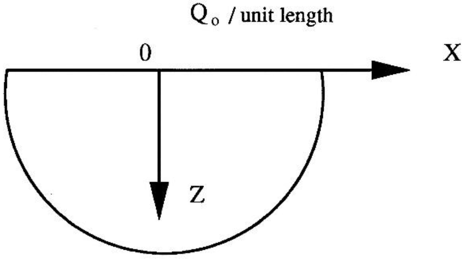
6. Concentrated Electric Charge Applied with the Free Boundary

Assume the following boundary conditions, see Figure 2:

Figure 2. Concentrated electric charge applicable to magneto-piezoelastic medium with free boundary.

Figure 2. Concentrated electric charge applicable to magneto-piezoelastic medium with free boundary.

$${\mathrm{\sigma }}_{zz}(x,0)=0\hspace{1em}{\mathrm{\sigma }}_{zx}(x,0)=0\hspace{1em}{D}_z(x,0)=Q_0\mathrm{\delta }(x)$$

(89)

Using these boundary conditions Equation (89) in the transformed space, we get

$${\mathrm{\xi }}^2(G_3{d}_{23}+G_2{d}_{22}+G_1{d}_{21})=0$$

(90)

$${\mathrm{\xi }}^2(G_3{d}_{33}+G_2{d}_{32}+G_1{d}_{31})=0$$

(91)

$${\mathrm{\xi }}^2(G_3{d}_{53}+G_2{d}_{52}+G_1{d}_{51})=Q_0.$$

(92)

Solving these equations results in the following solutions:

$$G_1=\frac{b_1}{{\mathrm{\xi }}^2},\hspace{1em}{G}_2=\frac{b_2}{{\mathrm{\xi }}^2},\hspace{1em}{G}_3=\frac{b_3}{{\mathrm{\xi }}^2}$$

(93)

where

$$b_1=-\frac{(d_{33}{d}_{22}-d_{32}{d}_{23})}{\Delta }{Q}_0,\hspace{1em}{b}_2=-\frac{(d_{31}{d}_{23}-d_{33}{d}_{21})}{\Delta }{Q}_0$$

(94)

$$b_3=-\frac{(d_{32}{d}_{21}-d_{31}{d}_{22})}{\Delta }{Q}_0$$

(95)

and $\Delta$ is given by Equation (54).

The complete solution is given by the following expressions:

$$u_x(x,z)=-{\displaystyle \sum _{j=1}^3}{\mathrm{\beta }}_j{b}_j{S}_j(x,z),\hspace{1em}{u}_z(x,z)={\displaystyle \sum _{j=1}^3}{\mathrm{\eta }}_j{b}_j{R}_j(x,z)$$

(96)

$$\mathrm{\phi }(x,z)={\displaystyle \sum _{j=1}^3}{\mathrm{\delta }}_j{b}_j{R}_j(x,z),\hspace{1em}{\mathrm{\sigma }}_{xx}(x,z)={\displaystyle \sum _{j=1}^3}{d}_{1j}{b}_j{R}_j^{\ast }(x,z)$$

(97)

$${\mathrm{\sigma }}_{zz}(x,z)={\displaystyle \sum _{j=1}^3}{d}_{2j}{b}_j{R}_j^{\ast }(x,z),\hspace{1em}{\mathrm{\sigma }}_{xz}(x,z)=-{\displaystyle \sum _{j=1}^3}{d}_{3j}{b}_j{S}_j^{\ast }(x,z)$$

(98)

$$D_x(x,z)=-{\displaystyle \sum _{j=1}^3}{d}_{4j}{b}_j{S}_j^{\ast }(x,z),\hspace{1em}{D}_z(x,z)={\displaystyle \sum _{j=1}^3}{d}_{5j}{b}_j{R}_j^{\ast }(x,z)$$

(99)

$$E_x(x,z)=-{\displaystyle \sum _{j=1}^3}{\mathrm{\delta }}_j{b}_j{S}_j^{\ast }(x,z),\hspace{1em}{E}_z(x,z)=-{\displaystyle \sum _{j=1}^3}{\mathrm{\alpha }}_j{\mathrm{\delta }}_j{b}_j{R}_j^{\ast }(x,z)$$

(100)

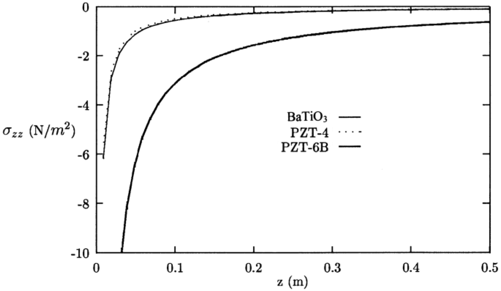
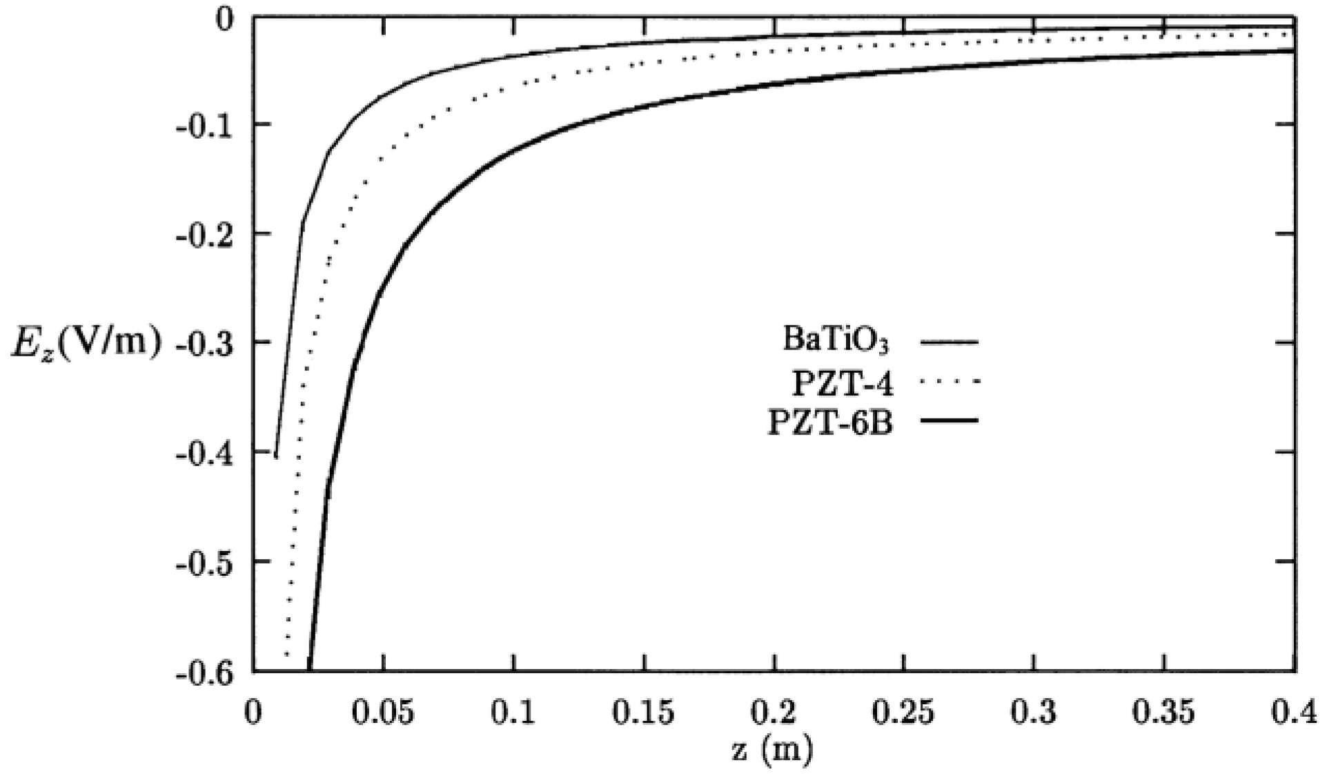
7. Results and Discussion

Table 1 presents the material properties of the three piezoelectric materials as well as the values of permeability and magnetic flux.

Table 1. Material Properties of Piezoelectric Materials.

Material property	BaTiO3	PZT-4	PZT-6B
$c_{11}({10}^{10}N/m^2)$	15.0	13.9	16.8
$c_{33}({10}^{10}N/m^2)$	14.6	11.5	16.3
$c_{12}({10}^{10}N/m^2)$	6.6	7.78	6.0
$c_{13}({10}^{10}N/m^2)$	6.6	7.43	6.0
$c_{44}({10}^{10}N/m^2)$	4.4	2.56	2.71
$e_{15}(C/m^2)$	11.4	12.7	4.6
$e_{31}(C/m^2)$	−4.35	−5.2	−0.9
$e_{33}(C/m^2)$	17.5	15.1	7.1
${\mathrm{\epsilon }}_{11}({10}^{-9}F/m)$	9.87	6.45	3.6
${\mathrm{\epsilon }}_{33}({10}^{-9}F/m)$	11.15	5.62	3.4

Table 1. Material Properties of Piezoelectric Materials.

Material property	BaTiO3	PZT-4	PZT-6B
$c_{11}({10}^{10}N/m^2)$	15.0	13.9	16.8
$c_{33}({10}^{10}N/m^2)$	14.6	11.5	16.3
$c_{12}({10}^{10}N/m^2)$	6.6	7.78	6.0
$c_{13}({10}^{10}N/m^2)$	6.6	7.43	6.0
$c_{44}({10}^{10}N/m^2)$	4.4	2.56	2.71
$e_{15}(C/m^2)$	11.4	12.7	4.6
$e_{31}(C/m^2)$	−4.35	−5.2	−0.9
$e_{33}(C/m^2)$	17.5	15.1	7.1
${\mathrm{\epsilon }}_{11}({10}^{-9}F/m)$	9.87	6.45	3.6
${\mathrm{\epsilon }}_{33}({10}^{-9}F/m)$	11.15	5.62	3.4

$$\begin{array}{ccc}{\text{μ}}_e& =& 0.0069115\frac{H}{m}\\ H_1& =& {10}^6\frac{A}{m}\end{array}\}\hspace{1em} \text{for}\hspace{0.17em}\text{all}\hspace{0.17em}\text{materials}.$$

The roots α₁, α₂,, α₃, corresponding to these three materials are presented in Table 2.

Table 2. Roots α₁, α₂,, α₃ for Piezoelectric Materials from Table 1.

Root	BaTiO3	PZT-4	PZT-6B
α1	(0.9596655583, 0)	(1.262398936, 0)	(0.5546941517, 0)
α2	(1.026584747, −0.2190857624)	(1.071962039, 0.165585358)	(1.014328206, 0)
α3	(1.026584747, 0.2190857624)	(1.071962039, −0.165585358)	(2.115922225, 0)

Table 2. Roots α₁, α₂,, α₃ for Piezoelectric Materials from Table 1.

Root	BaTiO3	PZT-4	PZT-6B
α1	(0.9596655583, 0)	(1.262398936, 0)	(0.5546941517, 0)
α2	(1.026584747, −0.2190857624)	(1.071962039, 0.165585358)	(1.014328206, 0)
α3	(1.026584747, 0.2190857624)	(1.071962039, −0.165585358)	(2.115922225, 0)

Figure 3, Figure 4, Figure 5 and Figure 6 show the variation of ${\mathrm{\sigma }}_{zz}$ and $E_z$ along the vertical axis of a magneto-piezoelastic solid which is subjected to a vertical line load of intensity 1.0 $N{m}^{-1}$ and an electric charge of intensity 1.0 $C{m}^{-1}$ at the top surface, as shown in Figure 1 and Figure 2.

The vertical stress and the vertical electric field along the z-axis are nearly indentical for all the three materials. Both ${\mathrm{\sigma }}_{zz}$ and $E_z$ decay rapidly with the vertical distance.

The solution presented due to an electric charge of 1.0 $C{m}^{-1}$ shows substantial difference for PZT-6B, which shows the largest magnitude for ${\mathrm{\sigma }}_{zz}$ and $E_z$, followed by PZT-4 and BaTiO₃. These results indicate that relatively large stresses are generated in PZT-6B compared with the other materials. The decay of the vertical stress and electric field with the depth is very rapid, as in the case of a vertical load.

Figure 3. Vertical stress in different magneto-piezoelastic solids due to a concentrated vertical line load of intensity 1.0 $N{m}^{-1}$.

Figure 3. Vertical stress in different magneto-piezoelastic solids due to a concentrated vertical line load of intensity 1.0 $N{m}^{-1}$.

Figure 4. Electric Field in different magneto-piezoelastic solids due to a vertical line load of intensity 1.0 $N{m}^{-1}$.

Figure 4. Electric Field in different magneto-piezoelastic solids due to a vertical line load of intensity 1.0 $N{m}^{-1}$.

Figure 5. Vertical stress in different magneto-piezoelastic solids due to a line electric charge of intensity 1.0 $C{m}^{-1}$ applied to the surface.

Figure 5. Vertical stress in different magneto-piezoelastic solids due to a line electric charge of intensity 1.0 $C{m}^{-1}$ applied to the surface.

Figure 6. Electric Field in different magneto-piezoelastic solids due to a line electric charge of intensity 1.0 $C{m}^{-1}$ applied to the surface.

Figure 6. Electric Field in different magneto-piezoelastic solids due to a line electric charge of intensity 1.0 $C{m}^{-1}$ applied to the surface.

8. Conclusions

The basic modeling aspects of the magneto-piezoelastic anistropic materials are developed in the present paper. Assumption of generally anisotropic properties of the materials under study is important from the practical point of view, and it renders the pertinent analysis significantly more complicated than in the simpler case of isotropic materials. Analytical modeling of these materials is essential for the design and application in smart composite structures incorporating them as actuating and sensing constituents.

The exact analytical solution is obtained for the anisotropic magneto-piezoelastic material using Green’s function method, boundary integral technique and Betti’s reciprocal theorem. The closed-form analytical solutions are derived for a number of boundary conditions for all components of the magneto-piezoelectric field. This includes the cases of the magneto-piezoelastic material subjected to vertical line load and electric charge at the surface; and the concentrated electric charge applied to the magneto-piezoelastic material with a free boundary.

As an application, a two-dimensional static plane-strain problem is dealt with to investigate the effect of magnetic field on piezoelectric material.

The analytical derivation is for the time-dependent problems. The numerical results are presented in particular case of static formulation for the two-dimensional magneto-electroelastic field of a piezoelectric solid subjected to a concentrated line load and an electric charge. Three different piezoelectric materials (BaTiO₃, PZT-4 and PZT-6B) are analyzed.

The obtained numerical solutions indicate a substantial dependence of the vertical stress and the electric field due to an electric charge on the constitutive properties as well as on the magnetic flux.

The solution due to an electric charge demonstrates substantial difference for PZT-6B, which shows the largest magnitude for ${\mathrm{\sigma }}_{zz}$ and $E_z$, followed by PZT-4 and BaTiO₃. These results indicate that relatively large stresses are generated in PZT-6B compared with the other materials. The decay of the vertical stress and electric field with the depth is very rapid, as in the case of a vertical load.

References

1. Bhatra, D.; Masud, M.G.; De, S.K.; Chauduri, B.K. Large magnetoelectric effect and low-loss high relative permittivity in 0–3 CuO/PVDF composite films exhibiting unusual ferromagnetism at room temperature. J. Phys. D Appl. Phys. 2012, 45, 485002. [Google Scholar] [CrossRef]
2. Bichurin, M.; Petrov, V.; Priya, S.; Bhalla, A. A multiferroic magnetoelectric composites and their applications. Adv. Condens. Matter Phys. 2012, 2012, 129794. [Google Scholar]
3. Srinivasan, G. Magnetoelectric composites. Annu. Rev. Mater. Res. 2010, 40, 153–178. [Google Scholar] [CrossRef]
4. Zhou, H.-M.; Li, C.; Xuan, L.-M.; Wei, J.; Zhao, J.-X. Equivalent circuit method research of resonant magnetoelectric characteristic in magnetoelectric laminate composites using nonlinear magnetostrictive constitutive model. Smart Mater. Struct. 2011, 20, 035001. [Google Scholar] [CrossRef]
5. Ju, S.; Chae, S.H.; Choi, Y.; Lee, S.; Lee, H.W.; Ji, C.-H. A low frequency vibration energy harvester using magnetoelectric laminate composite. Smart Mater. Struct. 2013, 22, 115037. [Google Scholar] [CrossRef]
6. Semenov, A.A.; Karmanenko, S.F.; Demidov, V.E.; Kalinikos, B.A.; Srinivasan, G.; Slavin, A.N.; Mantese, J.V. Ferrite-ferroelectric layered structures for electrically and magnetically tunable microwave resonators. Appl. Phys. Lett. 2006, 88, 033503. [Google Scholar] [CrossRef]
7. Lottermoser, T.; Lonkai, T.; Amann, U.; Hohlwein, D.; Ihringer, J.; Fiebig, M. Magnetic phase control by an electric field. Nature 2004, 430, 541–544. [Google Scholar] [CrossRef] [PubMed]
8. Shen, Y.; Mc Laughlin, K.L.; Gao, J.; Gray, D.; Shen, L.; Wang, Y.; Li, M.; Berry, D.; Li, J.; Viehland, D. AC magnetic dipole localization by a magnetoelectric sensor. Smart Mater. Struct. 2012, 21, 065007. [Google Scholar] [CrossRef]
9. Zhai, J.; Xing, Z.; Dong, S.; Li, J.; Viehland, D. Detection of pico-Tesla magnetic fields using magnetoelectric sensors at room temperature. Appl. Phys. Lett. 2006, 88, 062510. [Google Scholar] [CrossRef]
10. Hadjiloizi, D.A.; Georgiades, A.V.; Kalamkarov, A.L.; Jothi, S. Micromechanical model of piezo-magneto-thermo-elastic composite structures: Part I—theory. Eur. J. Mech. A-Solids 2013, 39, 298–312. [Google Scholar] [CrossRef]
11. Hadjiloizi, D.A.; Georgiades, A.V.; Kalamkarov, A.L.; Jothi, S. Micromechanical model of piezo-magneto-thermo-elastic composite structures: Part II—applications. Eur. J. Mech. A-Solids 2013, 39, 313–327. [Google Scholar] [CrossRef]
12. Rudykh, S.; Lewinstein, A.; Uner, G.; de Botton, G. Analysis of microstructural induced enhancement of electromechanical coupling in soft dielectrics. Appl. Phys. Lett. 2013, 102, 151905. [Google Scholar] [CrossRef]
13. Galipaeu, E.; Rudykh, S.; de Botton, G.; Ponte-Castaneda, P. Magnetoactive elastomers with periodic and random microstructures. Int. J. Solids Struct. 2014, 51, 3012–3024. [Google Scholar] [CrossRef]
14. Pan, E. Exact solution for simply supported and multilayered magneto-electro-elastic plates. Trans. ASME J. Appl. Mech. 2001, 68, 608–618. [Google Scholar] [CrossRef]
15. Smittakorn, W.; Heyliger, P.R. A discrete-layer model of laminated hygrothermopiezoelectric plates. Mech. Compos. Mater. Struct. 2000, 7, 79–104. [Google Scholar] [CrossRef]
16. Akbarzadeh, A.H.; Pasini, D. Multiphysics of multilayered and functionally graded cylinders under prescribed hygrothermomagnetoelectromechanical loading. Trans. ASME J. Appl. Mech. 2013, 81, 041018. [Google Scholar] [CrossRef]
17. Akbarzadeh, A.H.; Chen, Z.T. Hygrothermal stresses in one-dimensional functionally graded piezoelectric media in constant magnetic field. Compos. Struct. 2013, 97, 317–331. [Google Scholar] [CrossRef]
18. Kalamkarov, A.L. Composite and Reinforced Elements of Construction; Wiley: Chichester, NY, USA, 1992. [Google Scholar]
19. Khutiryansky, N.; Sosa, H. Dynamic representation formulas and fundamental solutions for piezoelctricity. Int. J. Solids Struct. 1995, 32, 3307–3325. [Google Scholar] [CrossRef]
20. Norris, A.N. Dynamic Green’s functions in anisotropic piezoelectric, thermoelectric and poroelasticity. Proc. R. Soc. Lond. A 1994, 447, 175–188. [Google Scholar] [CrossRef]