Article

The Instability Criterion for Bicrystal at Nanoscale

1
School of Materials Science and Engineering, Harbin Institute of Technology, Harbin 150001, China
2
National Key Laboratory for Precision Hot Processing of Metals, Harbin 150001, China
*
Author to whom correspondence should be addressed.
Metals 2018, 8(12), 986; https://doi.org/10.3390/met8120986
Submission received: 4 November 2018 / Revised: 15 November 2018 / Accepted: 20 November 2018 / Published: 24 November 2018

Abstract

:
Atomistic simulations are performed to predict the plastic yield using the instability criterion under thermal effect. The results show the instability criterion is applicable at low temperature (0~100 K) and invalid at a higher temperature (>200 K) due to the influence of thermal vibration. The tensile stress, minimum eigenvalue of matrix A, and atom configurations are compared to investigate the instability criterion in bicrytals. The instability criterion can successfully capture the plastic deformation initiation for bicrystal at 0 K.

1. Introduction

The yield strength is a very important mechanical property for engineering materials. Traditionally, those macro-yield criterions such as Tresca, Mises, double T2, τ2, and double shear yield criterion are basically formulated on the basis of macro mechanics. However, as the characterize sizes such as grain size are reduced down to the sub-micrometer. Even within the nanometer range, the yield criterions for the macro scale do not work anymore due to the nonnegligible contributions from grain boundaries (GBs) and other defects. Therefore, new yield criterion for plastic deformation in micro and nanoscale range needs to be established.
Many research studies had focused on the establishment and application of yield criterions at microscale for years. Milstein et al. [1,2] proposed a stability criterion based on the positive defined elastic constants at atomic scale. According to this crystal model, the shear movement of crystals had been successfully studied. This stability criterion was applied to investigate the stability of crystal models as well as the relationship between atomic structure and elastic properties of GBs. The elastic stability criterion of homogeneous lattice with uniformly distributed external loading was suggested by Wang et al. [3]. Its conditions depended explicitly on the applied stress involving only the elastic constants of the crystal. Their results revealed that crystal stability under ideal strength stress was not simply a question of material property. Cerny et al. [4] determined the upper limit of the mechanical strength by using the conditions for the stability criterion based on a more rigid analysis. An analytical formulation of the elastic limit was proposed by Van Vliet et al. [5], which predicts the location and slip character of a homogeneously nucleated defect in crystalline metals. Afterward, they extended the formulation on the atomic scale in the form of an energy-based, local elastic stability criterion known as the Λ criterion. They demonstrated that this approach could be incorporated efficiently into the computational methods such as molecular dynamics and finite-element models. Kolluri et al. [6] reported an fcc to hcp martensitic transformations in biaxially strained ultrathin films of fcc metals, which resulted from a dislocation slip. The onset of the phase transformation was identical with that of a shearing instability of the thin film.
However, the previously mentioned research studies have their limitations involving the concept of a continuous body scale, i.e., elastic constant and pressure, and it is difficult to transform it into a discrete atomic system. Furthermore, the fundamental hypothesis of uniform deformation is very important in defining the equivalently continuous variables at atomic level in the previously mentioned works. It is still questionable whether the criterion is valid in the case of heterogeneous deformation system. Kitamura et al. [7,8] and Miller et al. [9] proposed a new instability criterion sequentially related to only the interatomic potential independent of the order of the continuous body. This instability criterion has been widely used for different systems [10,11,12,13]. Yan et al. [10] proposed a mechanical instability criterion of arbitrary dislocation structures based on this method. It had been applied in the description of the onset of instability and the corresponding collapse modes of the veins and dislocation walls under external loading, which demonstrated the reliability of the method. Based on the instability criterion, Lich et al. [11] have presented an analytical method to allow rigorous descriptions of instability in arbitrary systems of ferroelectrics under finite electric fields and/or mechanical loading to achieve an understanding of the microscopic nature of instability in these systems.
In this paper, the study of the instability criterion is investigated to predict the plastic deformation initiation at high temperature for the first time. Based on the simplest structure, bicrystal has been widely used as the subjects in experiments [14] and simulations [15,16]. Therefore, three bicrystalline models are selected in this work to study the accuracy of the instability criterion in predicting the plastic yield.

2. Computational Methodology

2.1. Theory of Instability Criterion

In order to evaluate the unstable deformation of mono-crystals, Kitamura et al. [8] proposed the instability criterion at 0 K based on the potential energy variation of the whole system, which includes the second order differential of potential energy with respect to atomic coordinates.
At 0 K, the total energy of the system including N atoms is only determined by the position of atoms, which can be expressed by the equation below.
E = E ( R )
where the vector of the atomic position R = T ( R 1 , , R M ) and M is the degree of freedom.
When infinitesimal deformation Δ R occurs in the system, Equation (1) is expanded by using a Taylor series.
E ( R + Δ R ) = E ( R ) + m = 1 M E R m Δ R m + 1 2 m = 1 M n = 1 M 2 E R m R n Δ R m Δ R n +
Since the system is in equilibrium before deformation, m = 1 M E R m Δ R m = 0 . By omitting the terms above the second order, Equation (2) can be expressed by the equation below.
Δ E = E ( R + Δ R ) E ( R ) = 1 2 m = 1 M n = 1 M 2 E R m R n Δ R m Δ R n = 1 2 Δ R T A Δ R
where matrix A is a real symmetric matrix and its components are shown below.
A m n = 2 E R m R n   m ,   n   = 1 , , M
The matrix A can be orthogonally similar and diagonalized by the orthogonal matrix P = ( p 1 p M ) :
P 1 A P = P T A P = ( η 1 0 0 η M )
Where η 1 < η 2 < < η M .
By introducing the matrix Δ Q P 1 Δ R = ( Δ Q 1 , , Δ Q M ) , Equation (3) can be expressed by the formula below.
Δ E = 1 2 ( P Δ Q ) T A ( P Δ Q ) = 1 2 Δ Q T ( P T A P ) Δ Q = 1 2 m = 1 M η m ( Δ Q m ) 2
If all eigenvalues are positive, Δ E > 0 for arbitrary Δ Q . The system is turned from a low energy state to a high-energy state. This deformation cannot be emerged spontaneously. The system can recover to the original low energy state after the removal of external constraints. On the contrary, Δ E < 0 , the deformation can occur spontaneously. The yield behavior of materials is conformed to the latter condition, which means the yield starts with the minimum eigenvalue reduced to zero, i.e.,
η 1 0
This criterion is successfully applied in the simulation of tensile deformation of thin film and cracked body [7,8]. According to the criterion, when the minimum eigenvalue of matrix A in Equation (6) changes to a negative value, the system will approach a lower energy state, which represents the initiation of plastic deformation.

2.2. Derivation of the Minimum Eigenvalue of Matrix A

The total energy of system E can be expressed as the sum of the potential energy U and the work of the external load V.
E = U + V
Then substitute it into Equation (4).
A m n = 2 E R m R n = 2 U R m R n + 2 V R m R n
If we assume that the external load V is a constant load, then the following formula is true.
2 V R m R n = 0
Therefore, the expression of matrix A can be shown by the equation below.
A m n = 2 U R m R n
A Morse potential was adopted to describe the interatomic interaction. The function of potential energy is expressed as follows.
U = D { exp [ 2 A ( r 0 r ) ] 2 exp [ A ( r 0 r ) ] }
where D is the cohesive energy coefficient, A is the gradient coefficient of the potential energy curve, and r0 is the atomic distance at zero intermolecular forces. Then, take the first and second derivative of Equation (12), respectively.
U = 2 A D { exp [ A ( r 0 r ) ] exp [ 2 A ( r 0 r ) ] }
U = 2 A 2 D { 2 exp [ 2 A ( r 0 r ) ] exp [ A ( r 0 r ) ] }
In a system of an atomic model, the atomic center of mass is defined. Then the total potential energy of the system can be divided into two parts: the potential energy U1 between the mass center atom and other atoms and the potential energy U2 between all atoms except the mass center atom. The total potential energy U can be expressed by the equation below.
U = U 2 + U 1 = 2 i < j N U ( r i j ) + 2 j N U ( r 1 j )
The partial derivative of total energy of system E are taken by substituting with Equations (11) and (15).
E x m g = E 1 x m g + E 2 x m g = 2 j N U 1 j r 1 j r 1 j R 1 j R 1 j X 1 j g X 1 j g x m g + j m , 2 j N U m j r m j r m j R m j R m j X m j g X m j g x m g
where the m, n, I, j are the subscripts of the atom and g, h are the subscripts of components along x, y, or z. The Xijg stand for the distance between the ith and the jth atoms along the direction of the g component and rij stand for the distance between any two atoms in space.
X i j g = x j g x i g
R i j = 1 g 3 X i j g 2
r i j = R i j
By clarifying the expression of each variable, the values of the partial derivatives in Equation (16) can be obtained by the equations below.
r i j R i j = 1 2 R i j 1 2
R i j X i j g = 2 X i j g
Substitute the obtained partial derivatives into Equation (16) and calculate the potential energy between the mass center atom and other atoms U1 = E1:
  • when h = g, i.e., the atoms are in the same dimension.
    2 E 1 x m g x n h = 2 j N X 1 j g x m g X 1 j h x n h [ X 1 j g X 1 j h ( 2 U 1 j r 1 j 2 R 1 j 1 U 1 j r 1 j R 1 j 3 2 ) + 1 2 U 1 j r 1 j R 1 j 3 2 2 R 1 j X 1 j g X 1 j h ]
    (a) if m = j, X 1 j g x m g = X 1 j g x j g = 2 : (b) if mj, X 1 j g x m g = 1
  • when hg, i.e., the atoms are in different dimensions, 2 R m j X m j g X m j h = 0 . Therefore, the partial derivatives of E1 can be divided into two parts: 2 E 1 x m g x n h = summation item + additional item.
    • when m = n,
      2 E 1 x m g x n h = 2 j N [ X 1 j g X 1 j h ( 2 U 1 j r 1 j 2 R 1 j 1 U 1 j r 1 j R 1 j 3 2 ) ] + 3 [ X 1 m g X 1 m h ( 2 U 1 m r 1 m 2 R 1 m 1 U 1 m r 1 m R 1 m 3 2 ) ]
    • when mn,
      2 E 1 x m g x n h = 2 j N [ X 1 j g X 1 j h ( 2 U 1 j r 1 j 2 R 1 j 1 U 1 j r 1 j R 1 j 3 2 ) ] + j = m , n [ X 1 j g X 1 j h ( 2 U 1 j r 1 j 2 R 1 j 1 U 1 j r 1 j R 1 j 3 2 ) ]
Second, calculate the potential energy between all the other atoms except the center of mass U2 = E2.
2 E 2 x m g x n h = j m , 2 j N { 2 U m j r m j 2 ( r m j R m j ) 2 R m j X m j h X m j h x n h R m j X m j g X m j g x m g + U m j r m j 2 r m j R m j 2 R m j X m j h X m j h x n h R m j X m j g X m j g x m g + U m j r m j r m j R m j 2 R m j X m j g X m j h X m j h x n h X m j g x m g + U m j r m j r m j R m j R m j X m j g 2 X m j g x m g x n h } = j m , 2 j N X m j g x m g X m j h x n h { R m j X m j g R m j X m j h [ 2 U m j r m j 2 ( r m j R m j ) 2 + U m j r m j 2 r m j R m j 2 ] + U m j r m j r m j R m j 2 R m j X m j g X m j h }   = j m , 2 j N X m j g x m g X m j h x n h [ X m j g X m j h ( 2 U m j r m j 2 R m j 1 U m j r m j R m j 3 2 ) + 1 2 U m j r m j R m j 1 2 2 R m j X m j g X m j h ]
  • When h = g, 2 R m j X m j g X m j h = 2 . In this case, the following is true.
    (a)
    If nm, j = n,
    2 E 2 x m g x n h = [ X m n g X m n h ( 2 U m n r m n 2 R m j 1 U m n r m n R m n 3 2 ) + U m n r m n R m n 1 2 ]
    (b)
    If n = m,
    2 E 2 x m g x n h = j m , 2 j N [ X m j g X m j h ( 2 U m j r m j 2 R m j 1 U m j r m j R m j 3 2 ) + U m j r m j R m j 1 2 ]
  • When hg, 2 R m j X m j g X m j h = 0 . In this case, the following is true.
    (a)
    If nm, j = n,
    2 E 2 x m g x n h = [ X m n g X m n h ( 2 U m n r m n 2 R m j 1 U m n r m n R m n 3 2 ) ]
    (b)
    If n = m,
    2 E 2 x m g x m h = j m , 2 j N [ X m j g X m j h ( 2 U m j r m j 2 R m j 1 U m j r m j R m j 3 2 ) ]
    The expressions of all the above formulas are the values of matrix A.
    A = ( 2 E R 1 2 2 E R 1 R 2 2 E R 1 R i 1 2 E R 1 R i + 1 2 E R 1 R M 2 E R 2 R 1 2 E R 2 2 2 E R i 1 R 1 2 E R i 1 2 2 E R i + 1 R 1 2 E R i + 1 2 2 E R M R 1 2 E R M 2 )
Equation (30) is the expression of matrix A. Afterward, all the above expressions are written into the Matlab program (version. R2013b) [17] to process the calculation results of molecular dynamics in order to find the minimum eigenvalue and draw the eigenvectors of all molecules in the system at each moment.

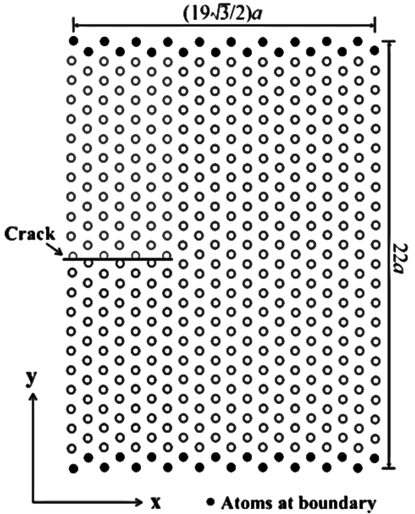
2.3. Simulation Methods

A Morse potential [18] of Al was adopted to describe the interatomic interaction due to its fast speed in calculating the minimum eigenvalue of matrix A. Among the function of potential energy of Equation (12), the three coefficients are given: D = 0.12, A = 2.35, and r0 = 2.86. The energy minimization process was carried out by a conjunctional gradient algorithm method after the model construction. For the minimization, the stopping tolerance for energy is set as 1.0 × 10⁻¹⁵, the stopping tolerance for force is 1.0 × 10⁻¹⁰ eV, the max iterations of minimizer is set as 5000, and the max number of force/energy evaluations is set as 100,000. The tensile loading was imposed on the fixed boundary step-by-step. The timestep was set as 0.001 ps. For each step, the simulation cell was stretched by a displacement of 0.01 Å with the following minimization process.
All atomic simulations in our work were performed by LAMMPS (13 April 2017, Sandia National Laboratories, Albuquerque, NM, USA) [19]. The AtomEye [20] was adopted as the visualization tool in our work. The local crystalline structure of each atom was computed according to the Ackland method [21]. In some cases, atoms with particular types would be deleted to facilitate the visualization of defects.

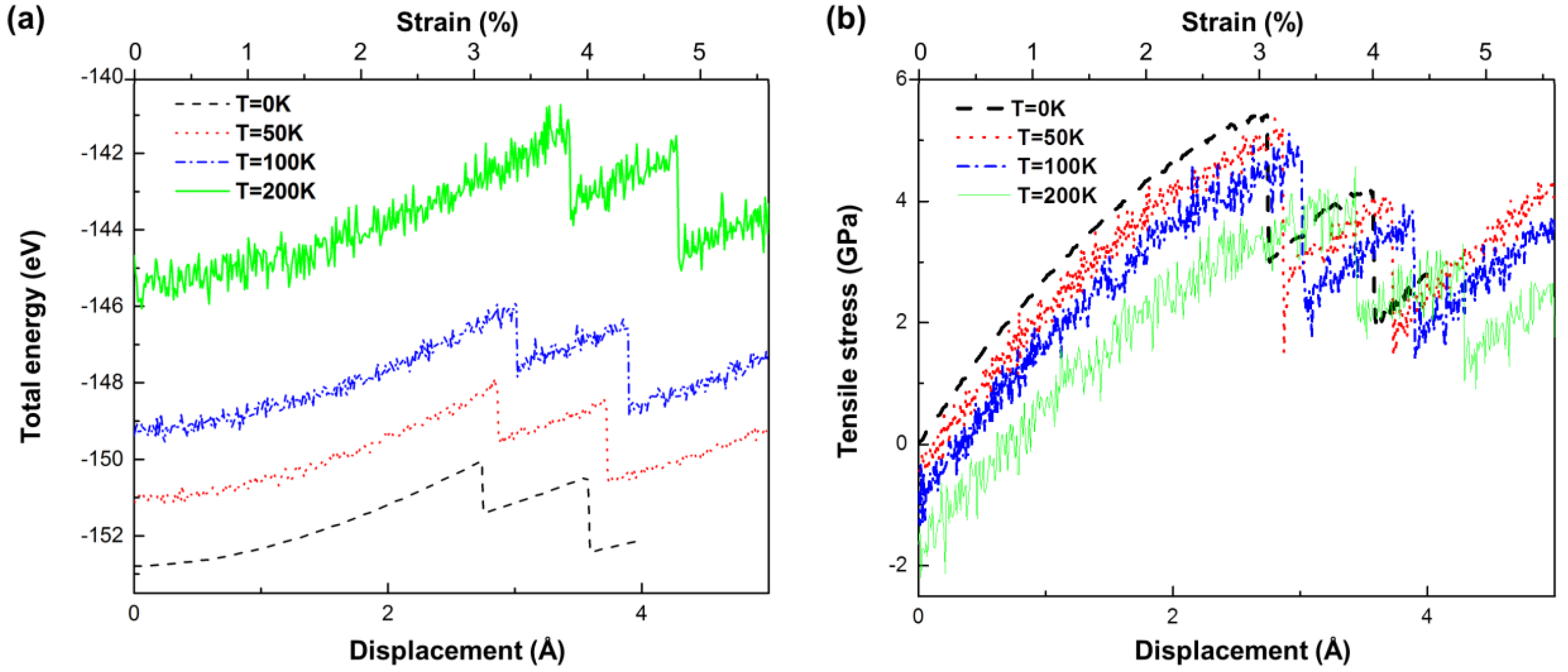
3. Yield Criterion under a Thermal Effect

The yield criterion based on energy variation is applied at absolute zero. When the temperature is 0 K, the total energy of the system only contains the potential energy. The increase of temperature makes all the atoms in the system vibrate thermally at the equilibrium position. By this thermal vibration, at a certain time, the energy of the system may become high enough to activate the plastic deformation. At 0 K, the energy variation of the system moves along the lowest energy trajectory. However, due to the existence of thermal vibration for a higher temperature, the energy variation will not move along the lowest energy trajectory. As the temperature increases, the amplitude of atomic thermal vibration at the equilibrium position will be larger and the yield deformation will be easier to achieve. In order to evaluate the mechanical instability of a system at a high temperature quantitatively, the variation of free energy must be considered instead of the potential energy and the statistical average value of the system must be taken. Therefore, the yield criterion at high temperature must be established on the basis of free energy variation. However, when the temperature is low, the thermal vibration has less influence. The instability points of free energy and potential energy are close to each other. As a result, the influence of the thermal vibration can be neglected.
In order to verify the application of the instability criterion above 0 K, a two dimensional model of a (111) close-packed plane of Al is established. The lattice parameter of Al is a0 = 4.047 Å and the minimum vertical distance between atoms is a = 1.427 Å. As shown in Figure 1, the model is 63 Å long and 47 Å wide including three (111) atomic layers. The crystallographic directions of the x, y, and z axis are [−110], [−1−12], and [111], respectively. The free boundary condition is applied along the x-axis and y-axis and the periodic boundary condition is applied along the z-axis. A crack is preset at the left of the model to control the dislocation nucleation site. The initial crack (solid line) is introduced by annihilating interaction between the atoms. The bottom of the model is fixed while a constant displacement δyy = 0.01 Å is imposed at the top. The reason why such a small two-dimensional model is selected is because it is time-consuming to calculate the eigenvalue by Matlab [22]. The two dimensional model is simulated at four different temperatures—0 K, 50 K, 100 K, and 200 K.
Figure 2a shows the curve of the total energy as a function of the tensile displacement. As the temperature increases, the total energy of system is increased as well. However, at each constant temperature, the energy variation trend is similar with zigzag fluctuations since the displacement increases. Figure 2b shows the curve of tensile stress as a function of the displacement. The tensile stress is increased with the decrease of temperature. For each constant temperature, the stress curve is similar as well. In addition, the turning points at stress curves are corresponding to those at energy curves for each constant temperature.
Using the yield criterion, the minimum eigenvalues of the two-dimensional model corresponding to the tensile displacement at different temperatures were obtained in Figure 3. From Figure 3a, the curves at T = 0 K, 50 K and 100 K are quite similar. When T = 0 K, the minimum eigenvalue becomes negative at a displacement of δyy = 2.754 Å. When T = 50 K, the minimum eigenvalue becomes negative at a displacement of δyy = 2.65 Å. When T = 100 K, the minimum eigenvalue become negative at a displacement of δyy = 2.46 Å. At these three temperatures, the drop points of minimum eigenvalue, tensile stress and total energy are nearly identical independently. As a result, this similar drop of a minimum eigenvalue indicates the initiation of plastic deformation at these three temperatures. As shown in Figure 3b, the minimum eigenvalues are disordered at 200 K. Therefore, it cannot predict the plastic yield.
In Table 1, the displacements at the first drop of energy, stress, and minimum eigenvalue at different temperatures are listed. For each temperature, the drop point of energy and stress are basically the same. At T = 0 K, the minimum eigenvalue becomes negative at δyy = 2.754 Å, which is similar to the drop point of energy and stress. This confirms the applicability and accuracy of the instability criterion at 0 K. As the temperature increases, the deviation of the drop point between stress and the minimum eigenvalue increases as well. The deviation is 0.21 Å at T = 50 K and 0.55 Å at T = 100 K. This deviation is in the acceptable range for T < 100 K. In addition, the instability criterion can be used to predict the yield behavior at 0~100 K. While at T = 200 K, the minimum eigenvalues are disordered and cannot accord with the instability criterion.
Figure 4 shows the atomic snapshots at different temperatures. When the displacement is 2.46 Å, the plastic deformation only occurs at T = 100 K. While, when the displacement increases to 2.65 Å, the plastic deformation occurs at T = 50 K as well.
From the above discussion, the instability criterion can be well applied in the prediction of plastic deformation initiation for the two dimensional models at 0~100 K. At the same tensile displacement, the minimum eigenvalue will become smaller with the increase of temperature. This means that the plastic yield will occur in advance. When the temperature is higher than 200 K, the instability criterion is invalid due to the disorder of minimum eigenvalues. This is because the atoms begin to vibrate around their original equilibrium position at a certain temperature. As the temperature increases, the thermal vibration will become stronger, the distance of the atoms deviated from the equilibrium position will become further, and the variation of the potential energy will become larger. Therefore, the potential energy of the system is composed of two parts: the potential energy variation caused by the tensile deformation and the potential energy variation caused by the thermal vibration. To discuss the applicability of the instability criterion, the effects of temperature are divided into three categories.
(a) When the temperature is high enough (greater than 300 K), the kinetic energy of the system has the same order of magnitude as the potential energy. To judge the mechanical instability, the free energy must be considered instead of the potential energy. Therefore, the microscopic plastic yield criterion based on the variation of the potential energy is not applicable.
(b) When the temperature is low enough (for example, 0~100 K), the variation of kinetic energy is very small relative to the potential energy (usually differ in two orders of magnitude), which can be neglected. Moreover, the amplitude of the atomic thermal vibration at the equilibrium position is not large. Therefore, the potential energy variation caused by thermal vibration is very small when compared with that caused by tensile deformation, which can also be neglected. Therefore, the potential energy variation of the system is controlled by the tensile deformation and the microscopic plastic yield criterion is applicable.
(c) When the temperature is in the intermediate state (about 200 K), the kinetic energy of the system is still very small and can be neglected. However, the amplitude of the atomic thermal vibration at the equilibrium position increases and the potential energy variation caused by this cannot be ignored. At this time, the energy variation of the system is not moving along the lowest energy trajectory and the microscopic plastic yield criterion cannot be applied.

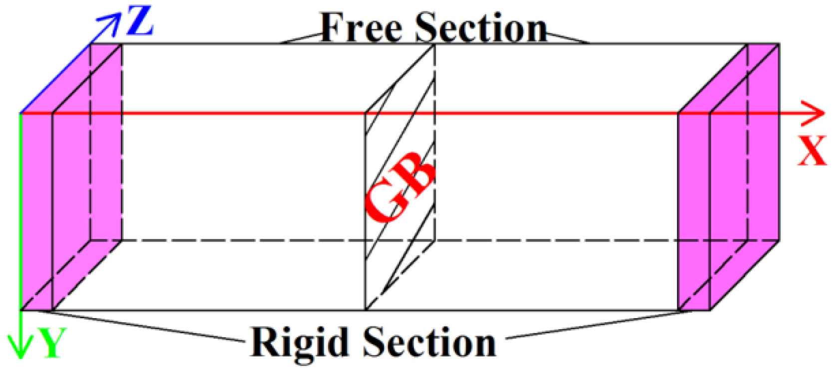
4. The Instability Criterion for Bicrystals

In order to study the accuracy of the instability criterion in predicting the plastic yield, bicrystalline models with distinct GBs are chosen for applying uniaxial tension at 0K. Three bicrystalline models with distinct GBs including the coherent twin boundary (CTB), the Σ5 (310) θ = 53.13° symmetric tilt grain boundary (STGB), and the Σ3 (33-2)/(7710) θ = 70.53° Φ = 10.02° asymmetric tilt grain boundary (ATGB) were constructed to study the accuracy of the instability criterion in bicrystals. First, a simulation box was established, as shown in Figure 5. Then the box was divided into two parts that represented the “left” and “right” grains. The Al atoms were added into the grains with different orientation. Thus, the plane between two grains was the GB with a specific misorientation angle. The parameters of the bicrystalline models were listed in Table 2.
The simulation cell was divided into two kinds of sections, i.e., the rigid section and the free section. Several layers of atoms on both sides of the box were maintained rigid, which was independent of any deformation of the simulation cell. Tensile loading was imposed on the rigid section. Since there was no constraint imposed on the free section, the atoms in this section were driven to deform by the displacement of the rigid section. Free boundary conditions were applied in the x direction and the periodic boundary condition is applied along the y-axis and the z-axis.

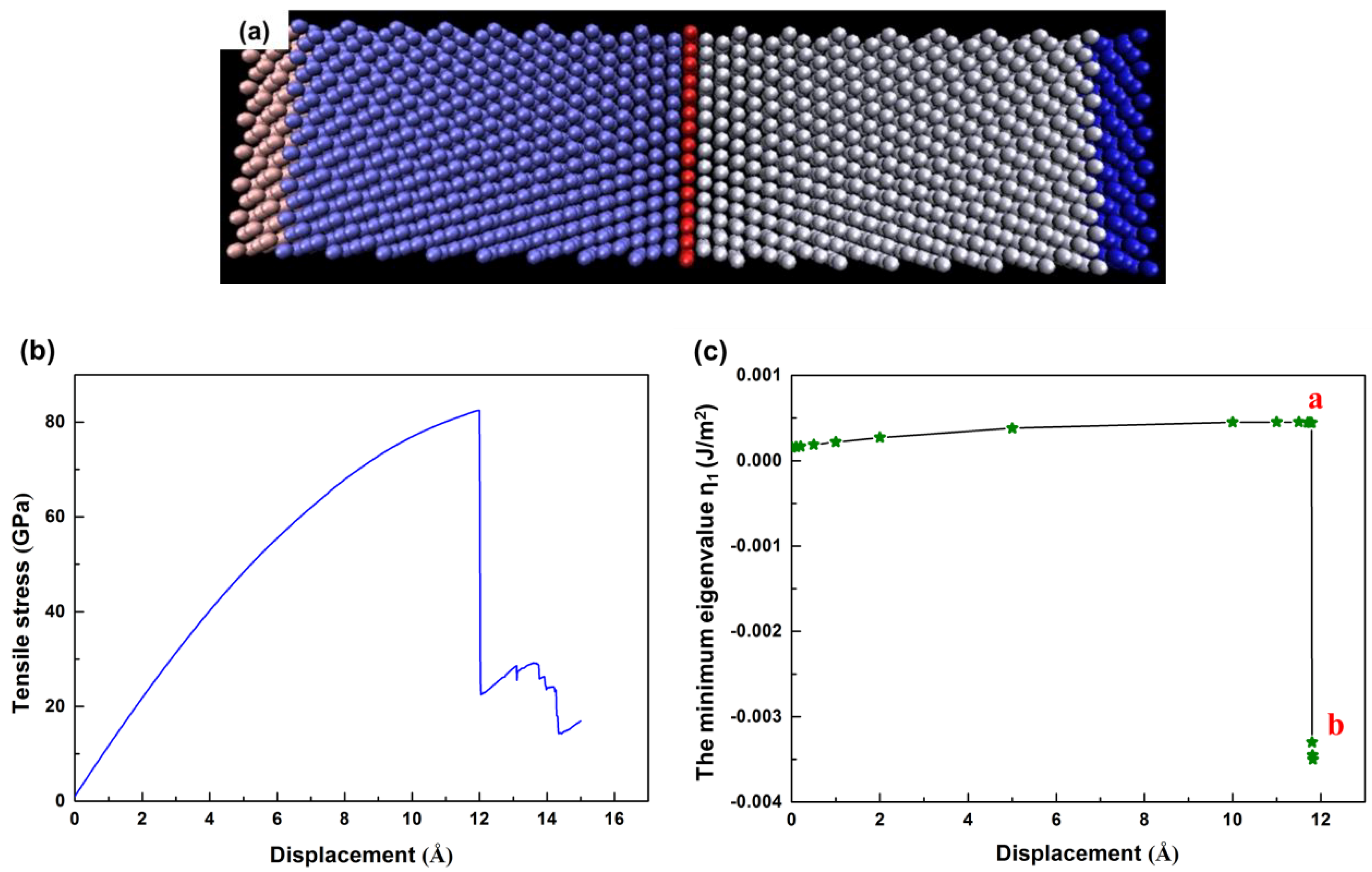
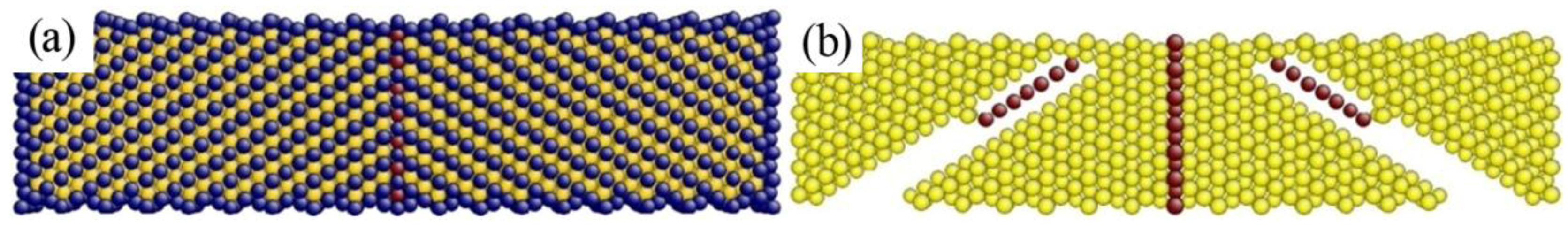
4.1. The Instability Criterion for a Bicrystal with a Coherent Twin Boundary

The atomic structure of model A with a CTB is shown in Figure 6a. To investigate the yielding behavior, the curve of tensile stress as a function of the tensile displacement is plotted in Figure 6b. Clearly, it can be found that the tensile stress increases uniformly with the increase of displacement until it reaches its maximum value of ~8 GPa at a displacement of 11.99 Å and then drops sharply, which implies the beginning of plastic deformation.
The calculated minimum eigenvalue (η1) of matrix A vs. tensile displacement for each loading step is shown in Figure 6c. The minimum eigenvalues (η1) of matrix A increases with the increment of tensile displacement with a small slope and then falls abruptly to a rather negative value at a displacement of 11.8 Å, which is approximate to the stress drop point in Figure 6b. According to the instability criterion, the eigenvalue drop to negative at this point, which denotes the initiation of plastic deformation.
In order to prove our predicted results, atomic configurations of point A and B, closely before and after the predicted occurrence of plastic deformation, are shown in Figure 7 and is analyzed in detail. At point A, where the displacement is 11.79 Å with a positive minimum eigenvalue (η1) 0.00044517 J/m2 of matrix A, the system is far from the plastic deformation in light of the instability criterion. From the atomic configuration snapshots in Figure 7a, no dislocations or stacking faults are observed. Therefore, both the instability criterion and atomic configuration snapshots confirm that the system is still in its elastic deformation stage at point A. At point B with a displacement of 11.81 Å, the minimum eigenvalue (η1) drops to −0.0034528 J/m2, which indicates the occurrence of plastic deformation is based on the instability criterion. As shown in Figure 7b, two dislocations emerge and emit from the free surfaces, which is in well agreement with the predicted results. In addition, the simulation cell exhibits a bamboo-like shape that is due to the steps at the free surfaces, which is caused by the exiting of dislocations. Thus, the instability criterion can be well applied in the prediction of plastic deformation initiation for bicrystalline models with a CTB.

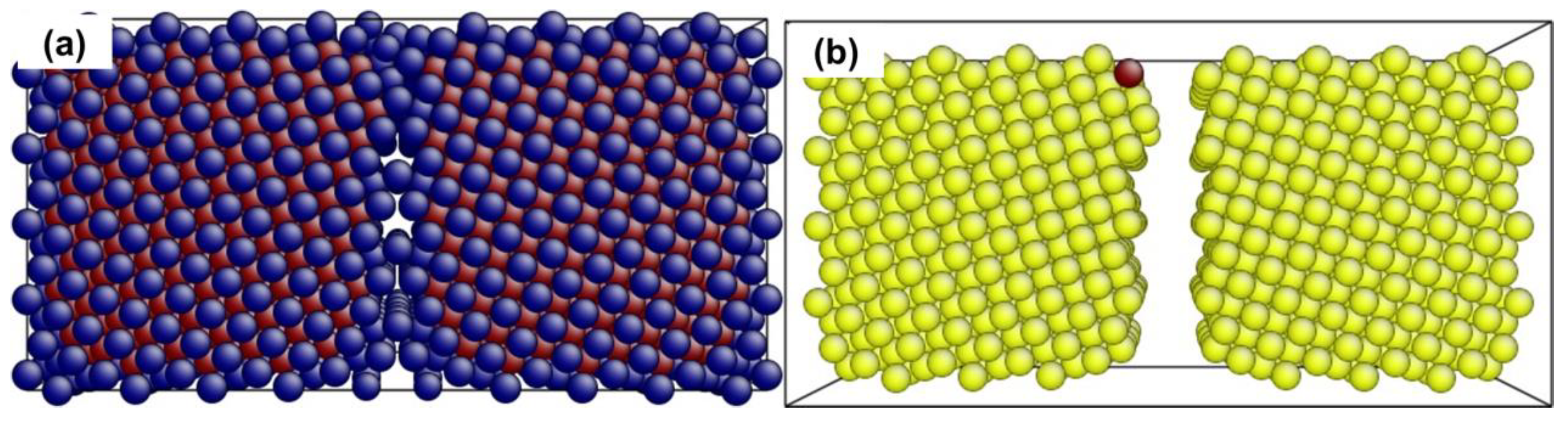
4.2. The Instability Criterion for a Bicrystal with a Symmetric Tilt Grain Boundary

The atomic structure of model B with a STGB is shown in Figure 8a. The simulation gives a tensile stress vs. tensile displacement curve, as shown in Figure 8b. The tensile stress of the simulation cell rises with displacement linearly before the displacement of 7.7 Å where the tensile stress drops abruptly due to plastic deformation.
Figure 8c shows the computed minimum eigenvalue (η1) of matrix A as a function of the displacement for each loading step. The minimum eigenvalue is always positive before it crosses the displacement axis at 7.1 Å and then becomes negative, which indicates the initiation of plastic deformation in light of the instability criterion. The crossover of the minimum eigenvalue at 7.1 Å is relatively close to the stress drop point in the stress-displacement curve. Compared with the simulation of model A with a CTB, atoms at STGB are easier to reconstruct, which are able to relax the system to an equilibrium state with a minimum energy. This gives rise to the decrease of the potential energy of the simulation cell. According to Equation (12), the eigenvalue will decrease with the increase of displacement, which is indicated in Figure 8c.
As shown in Figure 9, the atomic configurations of point A (7.1 Å) and B (7.2 Å) in Figure 8c are used to illustrate the changes in the simulation cell from a state of positive minimum eigenvalue to a state of negative minimum eigenvalue. As shown in Figure 9a (a positive minimum eigenvalue state), there are no new defects formed at this moment, which implies that the simulation cell remains in its elastic deformation stage. On the contrary, the fracture of bicrystal is observed in Figure 9 (a negative minimum eigenvalue state), which demonstrates the plastic deformation initiates at this point. As a conclusion, the plastic deformation predicted by the instability criterion is in good agreement with the stress-displacement curve prediction as well as the variations in atomic configurations. Therefore, the instability criterion can be well applied in the prediction of bicrystalline plastic deformation with a symmetric tilt boundary.

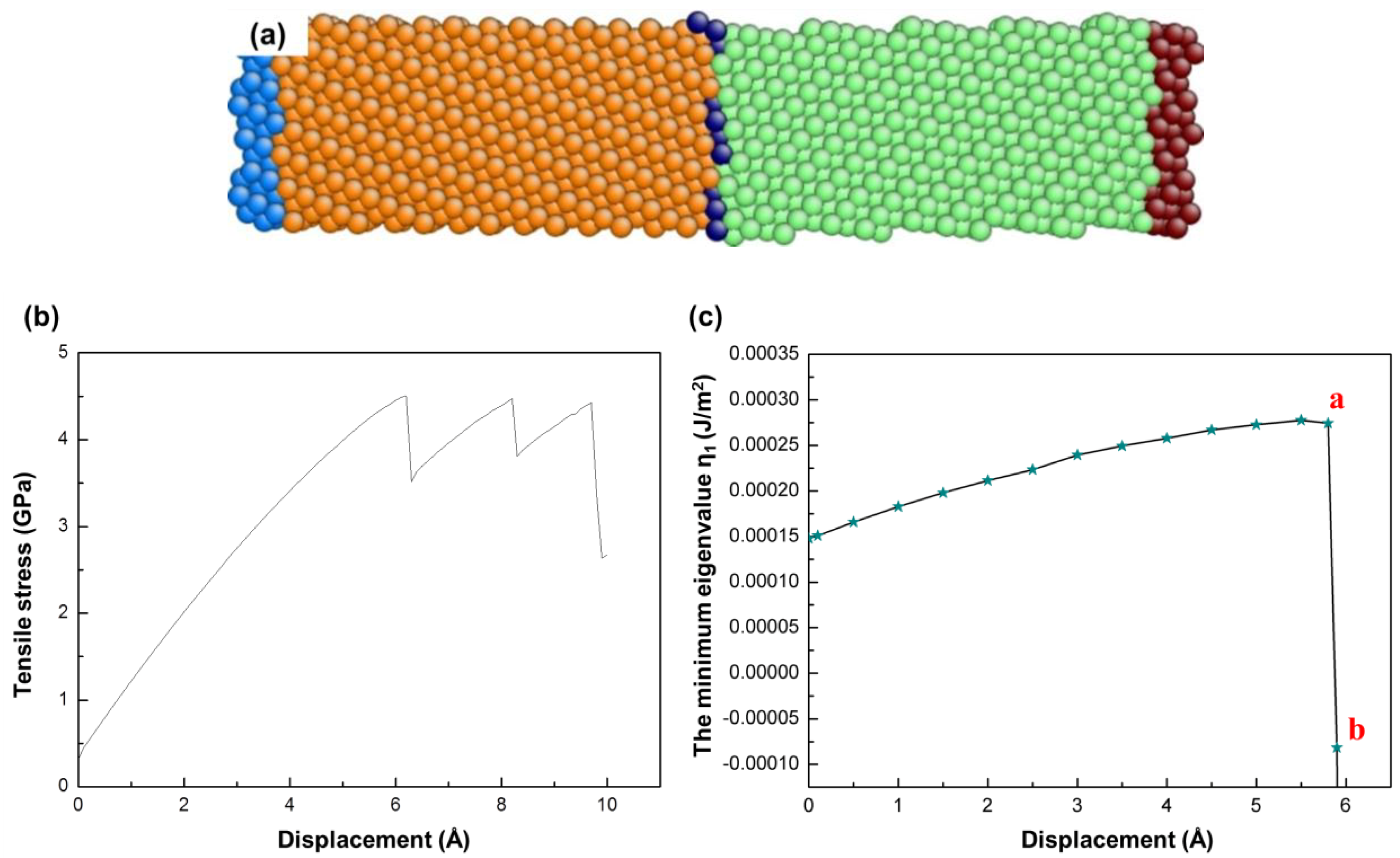
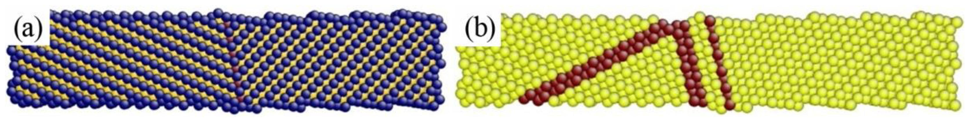
4.3. The Instability Criterion for a Bicrystal with Asymmetric Tilt Grain Boundary

The atomic structure of model C with a Σ3 (33-2)/(7710) ATGB is shown in Figure 10a. The curve of tensile stress as a function of the tensile displacement is shown in Figure 10b. It can be distinguished from the curve that the tensile stress increases linearly with the tensile displacement at its elastic stage. At a displacement of 6.2 Å, the tensile stress reaches its peak value, which is followed by a period of serrated flow and then drops abruptly. Thus, plastic deformation starts at the displacement of 6.2 Å.
The minimum eigenvalue (η1) of matrix A at each loading step as a function of tensile displacement is given in Figure 10c. The minimum eigenvalue increases continuously with loading displacement and then drops abruptly to a negative value. The variation of the minimum eigenvalue from a positive value to a negative value appears at the displacement of 5.9 Å, which is a signal of plastic yield, according to the instability criterion. It is in accord with that of the initially abrupt drop point in Figure 10b.
Similarly, the atomic configurations of point A and B in Figure 10c are shown in Figure 11 where point A has a positive minimum eigenvalue of 0.00027446 J/m2 at a displacement of 5.8 Å while point B has a negative minimum eigenvalue at a displacement of 6.3 Å. As shown in Figure 11a, there is no presence of newly formed defects at point A, which implies that the simulation cell still stays at an elastic stage. In Figure 11b, there are four layers of stacking faults found in the left grain of the simulation cell at point B, which is an indication of dislocation activities in the plastic deformation regime. As a result, the plastic deformation prediction of the instability criterion is in well agreement with the physics observed within the simulation cell as well as the prediction of the stress-displacement curve. Therefore, a conclusion can be drawn that the instability criterion can be introduced to predict the plastic deformation initiation of bicrystalline with ATGB.

5. Conclusions

In this paper, the instability criterion is introduced into the prediction of plastic yield under thermal effect. The results indicate that, when the temperature is low enough (T = 0~100 K), the instability criterion is applicable. While at higher temperature (T > 200 K), the instability criterion is invalid due to the influence of thermal vibration. In order to extend the criterion to higher temperatures, the free energy must be considered instead of the potential energy due to the existence of thermal vibration. Three bicrystalline simulation models with distinct GBs are constructed including CTB, STGB, and ATGB to investigate the accuracy of the instability criterion in the simplest polycrystalline deformation. Molecular statics simulation is used to perform all the simulations at 0 K. The displacements of the initiation of plastic deformation are found out according to the instability criterion and then they are compared with the results of the stress-displacement curve and the related atom configurations. Our results reveal that the instability criterion can successfully capture the plastic deformation initiation for bicrystals at 0 K.

Author Contributions

Conceptualization, L.Y.; Methodology, J.Z.; Software, J.Z.; Validation, C.X. and J.Z.; Formal Analysis, C.X. and J.Z.; Investigation, C.X.; Resources, C.X.; Data Curation, C.X.; Writing-Original Draft Preparation, C.X.; Writing-Review & Editing, L.Y.; Visualization, C.X.; Supervision, D.S. and B.G.; Project Administration, D.S. and B.G.; Funding Acquisition, L.Y.

Funding

This work was conducted under the funding of the National Natural Science Foundation of China (Grant No. 51675127).

Conflicts of Interest

The authors declare no conflict of interest.

References

  1. Milstein, F.; Huang, K. Theory of the response of an fcc crystal to [110] uniaxial loading. Phys. Rev. B 1978, 18, 2529–2541. [Google Scholar] [CrossRef]
  2. Milstein, F.; Hill, R. Divergences among the born and classical stability criteria for cubic crystals under hydrostatic loading. Phys. Rev. Lett. 1979, 43, 1411–1423. [Google Scholar] [CrossRef]
  3. Wang, J.H.; Li, J.; Yip, S.; Phillpot, S.; Wolf, D. Mechanical instabilities of homogeneous crystals. Phys. Rev. B 1995, 52, 12627–12635. [Google Scholar] [CrossRef]
  4. Cerny, M.; Sob, M.; Pokluda, J.; Sandera, P. Ab initio calculations of ideal tensile strength and mechanical stability in copper. J. Phys. Condens. Matter 2004, 16, 1045–1052. [Google Scholar] [CrossRef]
  5. Van Vliet, K.J.; Li, J.; Zhu, T.; Yip, S. Quantifying the early stages of plasticity through nanoscale experiments and simulations. Phys. Rev. B 2003, 67, 104105. [Google Scholar] [CrossRef]
  6. Kolluri, K.; Gungor, M.R.; Maroudas, D. Molecular dynamics simulations of martensitic fcc-to-hcp phase transformations in strained ultrathin metallic films. Phys. Rev. B 2008, 78, 195408. [Google Scholar] [CrossRef]
  7. Kitamura, T.; Umeno, Y.; Tsuji, N. Internal atomic stress near ∑5 tilt grain boundary in aluminium under tension. Model Simul Mater. Sci. Eng. 2003, 11, 839–849. [Google Scholar] [CrossRef]
  8. Kitamura, T.; Umeno, Y.; Tsuji, N. Analytical evaluation of unstable deformation criterion of atomic structure and its application to nanostructure. Comput. Mater. Sci. 2004, 29, 499–510. [Google Scholar] [CrossRef]
  9. Miller, R.E.; Rodney, D. On the nonlocal nature of dislocation nucleation during nanoidentation. J. Mech. Phys. Solids 2008, 56, 1203–1223. [Google Scholar] [CrossRef]
  10. Yan, Y.B.; Kondo, T.; Shimada, T.; Sumigawa, T.; Kitamura, T. Criterion of mechanical instabilities for dislocation structures. Mater. Sci. Eng. A 2012, 534, 681–687. [Google Scholar] [CrossRef] [Green Version]
  11. Lich, L.V.; Shimada, T.; Wang, J.; Kitamura, T. Instability criterion for ferroelectrics under mechanical/electric multi-fields: Ginzburg-Landau theory based modeling. Acta Mater. 2016, 112, 1–10. [Google Scholar] [CrossRef]
  12. Shimada, T.; Ouchi, K.; Ikeda, I.; Ishii, Y.; Kitamura, T. Magnetic instability criterion for spin-lattice systems. Comput. Mater. Sci. 2015, 97, 216–221. [Google Scholar] [CrossRef]
  13. Umeno, Y.; Shimada, T.; Kitamura, T. Dislocation nucleation in a thin Cu film from molecular dynamics simulations: Instability activation by thermal fluctuations. Phys. Rev. B 2010, 82, 104108. [Google Scholar] [CrossRef]
  14. Zaefferer, S.; Kuo, J.-C.; Zhao, Z.; Winning, M.; Raabe, D. On the influence of the grain boundary misorientation on the plastic deformation of aluminum bicrystals. Acta Mater. 2003, 51, 4719–4735. [Google Scholar] [CrossRef]
  15. Spearot, D.E.; Jacob, K.I.; McDowell, D.L. Nucleation of dislocations from [0 0 1] bicrystal interfaces in aluminum. Acta Mater. 2005, 53, 3579–3589. [Google Scholar] [CrossRef]
  16. Zhang, R.F.; Wang, J.; Beyerlein, I.J.; Germann, T.C. Dislocation nucleation mechanisms from fcc/bcc incoherent interfaces. Scr. Mater. 2011, 65, 1022–1025. [Google Scholar] [CrossRef]
  17. Lofberg, J. YALMIP: A toolbox for modeling and optimization in MATLAB. Optimization 2004, 3, 284–289. [Google Scholar]
  18. Girifalco, L.A.; Weizer, V.G. Application of the Morse Potential Function to Cubic Metal. Phys. Rev. 1959, 114, 687–690. [Google Scholar] [CrossRef]
  19. Plimpton, S. Fast parallel algorithms for short-range molecular-dynamics. J. Comput. Phys. 1995, 117, 1–19. [Google Scholar] [CrossRef]
  20. Li, J. AtomEye: An efficient atomistic configuration viewer. Model. Simul. Mater. Sci. Eng. 2003, 11, 173–177. [Google Scholar] [CrossRef]
  21. Ackland, G.J.; Jones, A.P. Applications of local crystal structure measures in experiment and simulation. Phys. Rev. B 2006, 73, 054104. [Google Scholar] [CrossRef]
  22. Sangiovanni, D.G. Inherent toughness and fracture mechanisms of refractory transition-metal nitrides via density-functional molecular dynamics. Acta Mater. 2018, 151, 11–20. [Google Scholar] [CrossRef]
Figure 1. The two dimensional tensile model.
Metals 08 00986 g001
Figure 2. (a) Plots of total energy vs. displacement. (b) Plots of tensile stress vs. displacement at different temperatures.
Metals 08 00986 g002
Figure 3. Plots of the calculated minimum eigenvalue (η1) of matrix A vs. displacement at (a) T = 0 K, 50 K, and 100 K. (b) T = 200 K.
Metals 08 00986 g003
Figure 4. Atomic structure at tensile displacement of (a) δyy = 2.46 Å. (b) δyy = 2.65 Å. (c) δyy = 2.754 Å at different temperatures.
Metals 08 00986 g004aMetals 08 00986 g004b
Figure 5. Schematic illustration of the bicrystalline model. The pink sections are rigid sections.
Metals 08 00986 g005
Figure 6. (a) Atomic structure of the bicrystalline model A with a coherent twin boundary. (b) Plot of tensile stress vs. displacement. (c) Plot of the calculated minimum eigenvalue (η1) of matrix A vs. displacement.
Metals 08 00986 g006
Figure 7. Atomic configuration of the simulation cell at (a) point A and (b) point B in Figure 6c. The atoms with unspecific coordination are deleted in (b) for a clear view of dislocation.
Metals 08 00986 g007
Figure 8. The computed minimum eigenvalue (η1) of matrix A vs. tensile displacement of the bicrystal simulation with a symmetric tilt grain boundary.
Metals 08 00986 g008
Figure 9. Atomic configurations of the simulation cell at (a) point A and (b) point B in Figure 8c.
Metals 08 00986 g009
Figure 10. (a) Atomic structure of the bicrystalline model C with an asymmetric tilt grain boundary. (b) Plot of tensile stress vs. displacement. (c) Plot of the calculated minimum eigenvalue (η1) of matrix A vs. displacement.
Metals 08 00986 g010
Figure 11. Atomic configuration of the simulation cell at (a) point A and (b) point B in Figure 10c.
Metals 08 00986 g011
Table 1. Displacement at the first drop point of energy, stress, and minimum eigenvalue at different temperatures.
Temperature (K)050100200
Displacement at the First Drop Point (Å)
Total energy2.742.853.013.42
Tensile stress2.742.863.013.41
Minimum eigenvalue2.7542.652.46disorder
Table 2. Detailed model parameters of the bicrystalline model.
ModelGBLattice OrientationLx (nm)Ly (nm)Lz (nm)Number of Atoms
Left GrainRight Grain
ACTBx [ 1 ¯ 1 ¯ 1 ¯ ]
y [ 112 ¯ ]
z [ 11 ¯ 0 ]
x [111]
y [ 112 ¯ ]
z [ 1 ¯ 10 ]
12.6173.4700.8321982
BSTGBx [ 3 ¯ 1 ¯ 0 ]
y [ 13 ¯ 0 ]
z [ 001 ]
x [ 1 ¯ 3 ¯ 0 ]
y [ 31 ¯ 0 ]
z [ 001 ]
6.1433.0712.0242570
CATGBx [ 332 ¯ ]
y [ 11 3 ]
z [ 11 ¯ 0 ]
x [ 7710 ]
y [ 5 ¯ 5 ¯ 7 ]
z [ 11 ¯ 0 ]
13.9493.2880.5721841

