Spreading Process Maps for Powder-Bed Additive Manufacturing Derived from Physics Model-Based Machine Learning

Abstract

The powder bed additive manufacturing (AM) process is comprised of two repetitive steps—spreading of powder and selective fusing or binding the spread layer. The spreading step consists of a rolling and sliding spreader which imposes a shear flow and normal stress on an AM powder between itself and an additively manufactured substrate. Improper spreading can result in parts with a rough exterior and porous interior. Thus it is necessary to develop predictive capabilities for this spreading step. A rheometry-calibrated model based on the polydispersed discrete element method (DEM) and validated for single layer spreading was applied to study the relationship between spreader speeds and spread layer properties of an industrial grade Ti-6Al-4V powder. The spread layer properties used to quantify spreadability of the AM powder, i.e., the ease with which an AM powder spreads under a set of load conditions, include mass of powder retained in the sampling region after spreading, spread throughput, roughness of the spread layer and porosity of the spread layer. Since the physics-based DEM simulations are computationally expensive, physics model-based machine learning, in the form of a feed forward, back propagation neural network, was employed to interpolate between the highly nonlinear results obtained by running modest numbers of DEM simulations. The minimum accuracy of the trained neural network was 96%. A spreading process map was generated to concisely present the relationship between spreader speeds and spreadability parameters.

1. Introduction

Powder-bed additive manufacturing has been rapidly evolving over the last decade, due in part to the design freedom it offers [1]. It is defined as the process of joining materials to make objects from 3D model data, usually layer upon layer [2]. The process consists of layer by layer spreading of a powdered material and selective fusion or binding of the spread layer to produce 3D objects. State of the art 3D printed parts have microscopic defects, at layer-level, like porosity, roughness and over or under fused/bound particles and macroscopic, at part level, defects like poor surface finish, voids, dimensional inaccuracy and shear-induced deformation. Few of these defects are directly related to the spreading step in powder-bed additive manufacturing (AM) [3,4,5,6,7,8,9,10,11,12,13,14].

1.1. Powder Spreading Studies

Authors of this study have previously defined powder spreadability as the ease with which a powder will spread under a set of load conditions [15] and have introduced four spread layer properties which can be used to quantify spreadability—mass of powder retained in the sampling region after spreading, spread throughput, roughness and porosity of the spread layer [4]. Spread throughput refers to the volume of powder spread per unit width of spreader per unit time and is indicative of speed of printing with respect to spreading [4]. Roughness of the spread layer is based on the RMS value of the topography of the spread layer [4]. Porosity of the spread layer represents the ratio of volume of pores to the volume of the spread layer cuboid or alternatively one minus the ratio of volume of powder particles to the volume of the spread layer cuboid [4]. Snow et al. [3] have developed a similar spreadability metric comprising of the percent build plate coverage, the powder deposition rate and the rate of change of the avalanche angle. There is a consensus in the literature on the applicability of the Discrete Element Method (DEM) to study the problem on AM powder spreading [5,6,7,8,9,11,12,13,14]. DEM was used by Haeri in 2017 [10] to optimize the shape of blade-like spreaders to minimize spread layer defects. Few studies [16,17,18] have tried to use high energy X-rays to visualize the powder spreading in situ, however these studies had to make use of a thin slice of powder in direction perpendicular to the X-rays due to the low penetration depth of view offered by X-rays. Thereby these studies were unable to study the full 3D nature of the powder spreading problem.

1.2. AM Machine Learning Studies

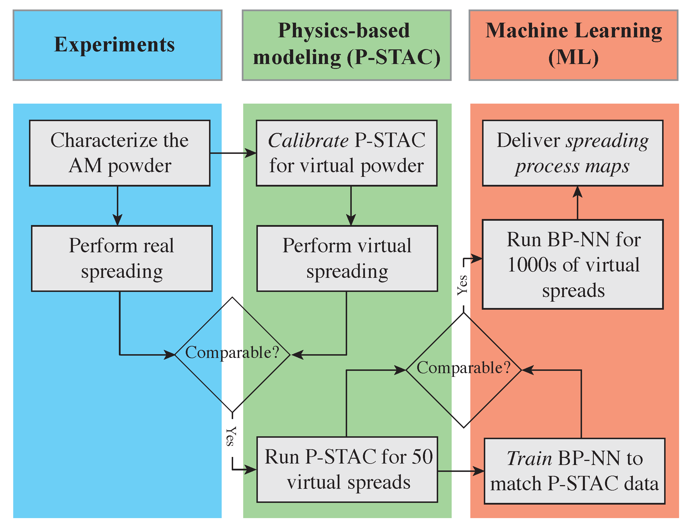
Recent advances in the field of data science and machine learning (ML) have resulted in works combining ML and AM. Everton et al. [19] review in situ analysis for AM processes and highlight key technologies for process control in metal AM. The big data from sensors is mentioned to be the bottleneck for developing effective closed-loop process control. Bumann et al. [20] provide a review of state-of-the-art AM ML studies. ML studies are classified into studies used to optimize AM process parameters, to improve object properties, to enable process monitoring and closed-loop process control and to improve digital security. An overview of AM informatics—science of managing AM data across its lifecycle is provided in Reference [21]. A review of descriptive, predictive and prescriptive ML studies in continuum materials mechanics—process parameters, microstructure, mechanical properties and performance is provided in Reference [22].

Kamath in 2016 [23] introdced an iterative synergistic approach involving different levels of complexity in experiments and simulations to optimize the process parameters of a selective laser melting machine to print dense 316L SS parts (>99% dense). Data mining and statistical inference were used in this study.

A data mining approach in real-time measurement for polymer additive manufacturing was studied in Reference [24]. Brian et al. [25] developed an autonomous objective system devoid of subjective human judgement, to implicitly characterize powder micrographs as a distribution of local image features. The system was capable of classifying powders having different distributions of particle size, shape and surface texture with an accuracy of over 95%. The ML system was also useful in quantitatively identifying representative and atypical powder images. A hybrid ML algorithm comprised of clustering (unsupervised learning) and SVM (supervised learning) was developed to manage design knowledge and help inexperienced designers to explore AM-enabled design freedoms in Reference [26]. Uhlmann et al. [27] provided data driven predictions for condition monitoring and clustering of data from an SLM machine.

Gu et al. [28] proposed design of hierarchical materials using machine learning and finite element analysis. Additionally, this work showed that machine learning can be used as an alternative method of coarse-graining, with the ability to analyze and design materials without the use of full microstructural data. A random forests-based predictive modeling approach to predict surface roughness of parts produced using FDM (fused deposition modeling) was proposed in Reference [29]. Gorbert et al. [30] developed in situ defect detection strategy for PBF AM using in situ sensor data from a DSLR camera and ex situ ground truth defect data from CT images of the 3D printed part. The lighting condition dependent strategy was shown to detect defects of incomplete fusion, cracks and porosity with 80% accuracy. Bessa and Pellegrino [31] developed a data-driven framework comprising of Design of Experiments (DoE), computational analyses, machine learning and multi-objective optimization to develop design charts and find optimal design of Triangular Rollable And Collapsible (TRAC) boom. This type of structure consists of two thin cylindrical shells of uniform thickness and has an approximately triangular cross-section, consisting of single-thickness transversely curved flanges and a double-thickness flat web. A multi-scale convolutional neural network was used to detect anomalies in laser powder bed fusion systems in Reference [32].

Machine learning techniques were investigated for the continuous printing speed modeling, selection and optimization for Continuous Liquid Interface Production (CLIP) a vat photopolymerization based additive manufacturing in Reference [33]. Siamese Network was shown to be more effective at capturing features for identifying the optimum manufacturing speed. In Reference [34], a data-driven and ensemble learning-based predictive model was developed to predict surface roughness of parts printed using fused filament fabrication (FFF). The condition monitoring data, which served as input to the predictive model, was obtained using multiple sensors. Zhang et al. [35] used deep learning in the form of LSTM NN (long short-term memory neural network) and layer-wise relevance propagation to predict tensile strength of dog-bone specimens printed using fused deposition modeling (FDM). The tensile strength of the final specimen was predicted as a function of the contribution from each of the printing layers, measured using in-process sensing of temperature and vibration data, fused together with process parameters and material property [35].

However, none of these studies provide intelligent closed-loop control of 3D printers with regards to the spreading step. The present computational study proposes to solve this by using ML to develop physics model-based surrogate model for a high-fidelity, computationally expensive physics-based model of the spreading process. To the best of our knowledge, no study exists that tries to elucidate the spreading process to obtain process maps by following the methodology described in Section 2. Predictions from the machine learning model are discussed in Section 3, followed by conclusions in Section 4.

2. Methodology

It is challenging to study the spreading step of powder-bed AM, not only experimentally but also computationally. It is difficult to study this experimentally as the in situ measurements of layer defects are challenging. Physics-based computational modeling of the spreading step is highly expensive due to the need to simulate hundreds of thousands of powder particles. Therefore, a synergistic, three-step approach as shown in Figure 1 was employed to study the powder spreading step in powder-bed AM. This approach is the same as the one proposed by authors in an earlier study [36] but improves the fidelity of the physics-based model by accounting for realistic particle size distribution (PSD) of an industry-grade Ti-6Al-4V and roughness of the spreading substrate. The first step involves the characterization of the AM powder using a powder rheometer developed by Freeman Technology, U.K. and using the data for calibrating a ‘virtual powder’ which behaves similar to the real AM powder as discussed in the previous work of authors [15]. The second step involves the spreading simulation study of this rheometry-validated virtual powder and comparison to the real spreading, as discussed in [4]. Finally, referring to Figure 1, the simulation data is used to develop a physics model-based surrogate model of the physics-based model. This model is then used to generate, what the authors refer to as, a spreading process map which maps the spreader speeds to the spread layer defects and spread throughput. The present study is directed towards elaborating parts of the second and third step of this methodology and discussing the results obtained using these steps.

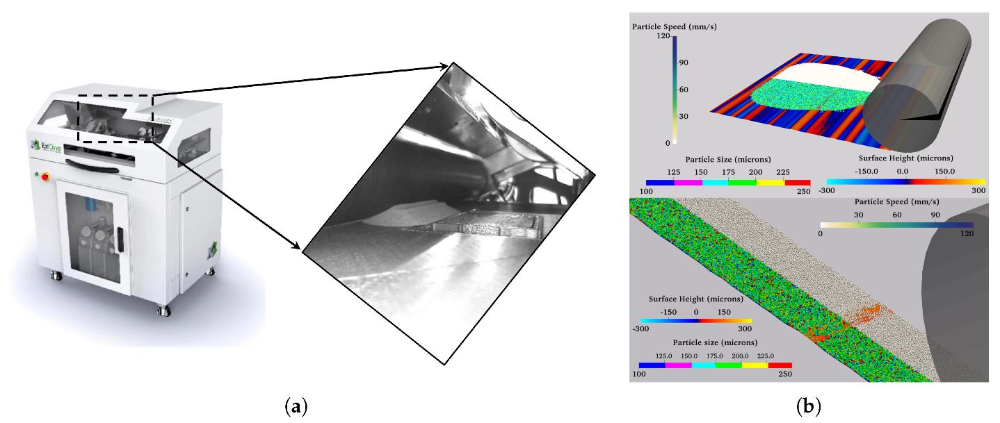
2.1. Physics-Based Polydispersed DEM Model

The authors have developed an in-house multiphysics computational modeling platform known as the Particle-Surface Tribology Analysis Code (P-STAC), which has a DEM module as its particle dynamics simulation tool. The DEM model is based on the one developed by Cundall and Strack [37] and has been validated in an earlier work by the authors [15]. It was shown by the authors of this study that it is important to account for a realistic particle size distribution while performing virtual powder spreading [4]. This validated polydispersed model will be used in the present study.

P-STAC is used to simulate single layer spreading as seen in a retrofit to a commercial powder-bed 3D printer, developed by ExOne, USA, refer Figure 2a. The spreading substrate as seen in the inset in Figure 2a was additively manufactured using a powder-bed fusion printer and the spreading of a single layer of powder was carried out over it. Sample simulation output is shown in Figure 2b. Here the front half of the particles has been color-coded by particle size and the back half has been color-coded by particle speed. The DEM simulations had particles of Ti-6Al-4V with an assumed normal of Gaussian particle size distribution (PSD) in the range of 100–250 μm. The real AM powder also had particles in the range of 100–250 μm. The topography of the spreading substrate is also shown. The roughness of the spreading substrate, $S_q$ is 79 microns. The spreader is able to spread a dense layer of powder everywhere except where the spreading substrate has steep protrusions. These defects of partial coverage result in the porosity of the spread layer and can eventually result in voids in the final 3D-printed part. These voids will act as stress concentration points and thereby a source of part failure [38]. The polydispersed DEM simulations can be used to correct such defects by altering the spreader speeds.

Spread Layer Characterization

The polydispersed DEM model allows one to predict spread layer properties which otherwise might be difficult to measure experimentally. These properties include mass of the powder in the sampling region $M_s$, spread throughput $Q_s$, roughness of the spread layer $R_q$ and porosity of the spread layer $\varphi$. The sampling region is a square area of 25 mm by 25 mm located in the central region of the spread layer. The mathematical description of these properties, as reproduced from Reference [4] is as follows:

Figure 3 shows a generalized schematic of the side view of a spread layer i. The heights of the previously 3D-printed (i.e., spread and fused) layer (i − 1) are denoted by b’s while the heights of the post-spread surface (consisting of fresh powder particles) are denoted by h’s. In other words, b’s are the heights measured by a virtual profilometer before the fresh powder was spread and h’s are the heights measured by a virtual profilometer after the powder was spread. Notice the point of layer (i − 1) denoted by $b_3$ where no powder was spread due to a steep peak. This point will be also registered as an h point (i.e., $h_3$) for layer i while calculating its roughness. In the present study, points at the intersection of randomly distributed 1000 × 1000 lines over the surface area of the sampling region were used for the measurements of h’s and b’s.

The average height of layer (i − 1), denoted by $b_{avg}$ and that of layer i denoted by $h_{avg}$, can be given by:

$$b_{avg}=\frac{{\sum }_{i=1}^L{b}_i}{L}$$

(1)

$$h_{avg}=\frac{{\sum }_{j=1}^M{h}_j}{M}$$

(2)

The average spread layer thickness can then be given by:

$$th{k}_{avg}=h_{avg}-b_{avg}$$

(3)

The quantities which answer the above four questions can be mathematically obtained as follows. The mass of powder particles in sampling region, $M_s$ can be expressed as

$$M_s=\frac{\pi \rho }{6}\sum _{k=1}^N{{\varphi }_k}^3$$

(4)

Here N is the number of powder particles in the sampling region of $L_x$ by $L_y$. While ${\varphi }_k$ is the diameter of the kth particle and $\rho$ is the material density of powder particles.

Volume of powder spread per unit time per unit width of spreader, $Q_s$ can be expressed as

$$Q_s=U·th{k}_{avg}$$

(5)

where, $th{k}_{avg}$ is given by (3) and U is the translation speed of the spreader.

Roughness of the spread layer, $R_q$ can be expressed as

$$R_q={\left[\frac{{\sum }_{j=1}^M{(h_j-h_{avg})}^2}{M}\right]}^{\frac{1}{2}}$$

(6)

And finally, porosity of the spread layer, $\Phi$ can be expressed as

$$\Phi =\left[1-\frac{M_s}{\rho L_x{L}_y(4R_q)}\right]·100\%$$

(7)

Spread layer sampling regions for a constant spreader translation speed and varying rotational speed are shown in Figure 4. The variation in spread layer properties is not easily seen however the spread layer properties do exhibit quite a lot of variation for these three spreader speeds. Refer to Section 3 for details.

2.2. Design of Simulations for Virtual Spreading

Physics-based simulations with the polydispersed DEM module of P-STAC can be used to provide predictions about the spread layer characteristics by varying the translation and rotational speeds of the spreader. However these simulations are computationally expensive. It can take on an average 2 h to run a single layer spreading physics-based simulation with 435,000 DEM particles having sizes in the range of 100–250 μm. Thus it is not feasible to cover the entire process parameter space at refined intervals using the polydispersed DEM model. However, a Design of Simulations (DoS), akin to Design of Experiments (DoE), can be carried out by sampling the process parameter coarsely and then training a machine learning model to regress between the results obtained by the physics-based model. The different parameters for such a DoS of spreading simulations are summarized in

Table 1. Design of Simulations (DoS) for virtual spreading of polydispersed particulate media.

Parameter	Range of Values
Spreader diameter (mm)	30
Spreader length (mm)	70
Spreader translation speed, U (mm/s)	40, 55, 70, 85, 100
Spreader rotation speed, $\omega$ (rad/s)	0, 5, 10, 15, 20, −5, −10, −15, −20
Substrate roughness $S_q$ (μm)	79

. Spreading cases with no roller rotation and roller rotating in clockwise direction (negative values), resulted in deposition of 2–3 powder layers over a single pass of spreader as opposed to a single layer of particles with single pass of anticlockwise rotating roller. The physics-based simulation results, as seen in Figures 6–9 (blue and black points), are highly non-linear. To gain a better understanding of the effect of these speeds on the spread layer properties $M_s$, $Q_s$, $R_q$ and $\Phi$, machine Learning (ML) enabled surrogate modeling can be employed to regress between these highly non-linear data points as described in the next sub-section.

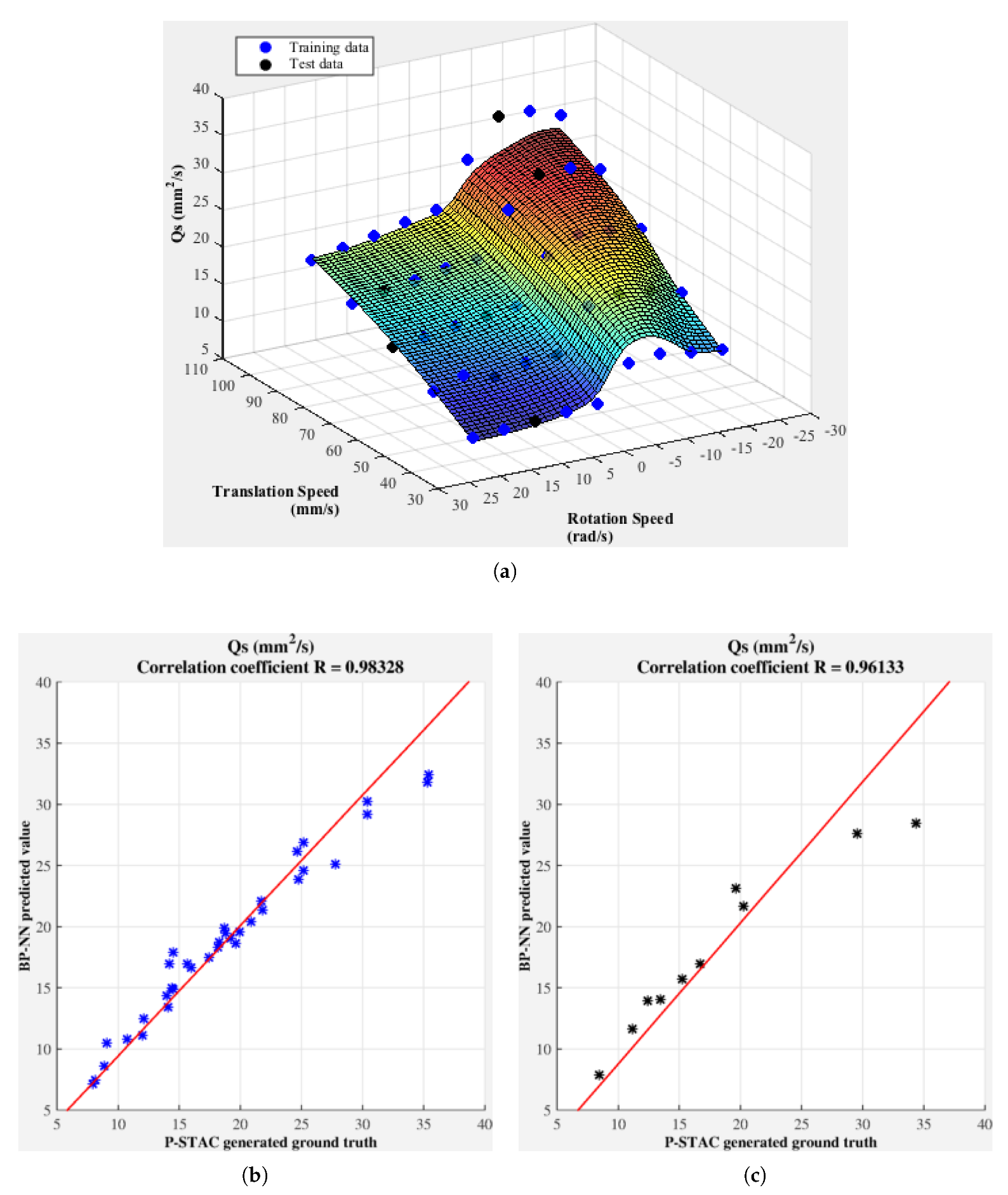
2.3. Physics Model-Based Machine Learning Enabled Surrogate Model

A schematic of a Back Propagation Neural Network (BP-NN) with 2 inputs and 4 outputs, is shown in Figure 5. A single hidden layer was used in this study. The topology of BP-NN used in the present study is shown in

Table 2. Back Propagation Neural Network (BP-NN) parameters.

Parameter	Value	Parameter	Value
Number of training samples	35	Activation function for hidden layer	Sigmoid
Number of test samples	10	Activation function for output layer	Linear
Number of hidden layers	1	Learning rate $\alpha$	0.0001
Number of hidden nodes	200	L2-regularization parameter $\lambda$	0.1

. This topology is based on the neural network used in an earlier study by the authors [36]. This neural network creates a map between the spreader speeds as the inputs and spread layer properties as the outputs. Sigmoid function is used as the activation function for the hidden layer and L-2 regularization is used to avoid overfitting. The data for training and testing the neural network is obtained by running the polydispersed DEM model by following the DoS described in Section 2.2. The data from physics-based simulations is devoid of noise which can occur in data obtained using physical sensors and thus the topology of the neural network is much simpler and shallower than what might be required for a neural network trained on the data from physical experiments. The results from the ML surrogate model are discussed in the next section.

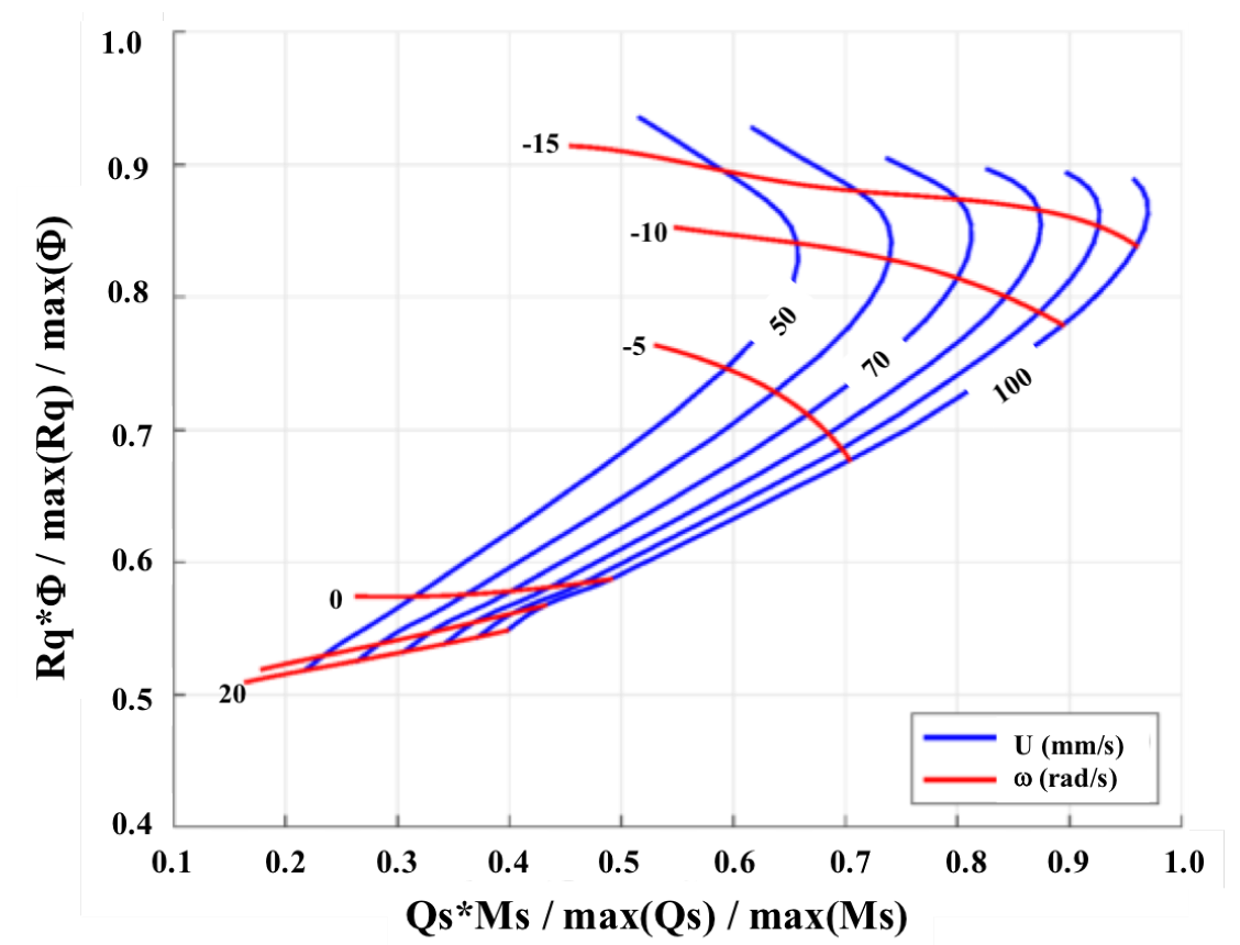
3. Results and Discussion

Regression results from the final BP-NN with parameters listed in Table 2 are shown in Figure 6, Figure 7, Figure 8 and Figure 9 for spreading simulations over a rough substrate ($S_q$ = 79 μm). Throughout, blue dots represent training data and black dots represent test data. The numerical values of the spread layer properties for the 3 sampling regions shown in Figure 4, can be seen in Figure 6, Figure 7, Figure 8 and Figure 9 (points on back-most edge of the surface corresponding to U = 100 mm/s). These properties show a non-linear dependence on the speeds of the spreader. Such shearing flow of powders with polydispersity results in percolation-type segregation [39,40].

The surfaces predicted by this BP-NN, refer sub-figure (a) of Figure 6, Figure 7, Figure 8 and Figure 9, nicely blanket the simulation data points, both training and test data points, generated via DoS. In these surface plots, dark blue corresponds to the lowest values and dark red corresponds to the highest values. Also shown is the correlation coefficient R between P-STAC simulation results and BP-NN predicted results (b) and (c) sub-figures of Figure 6, Figure 7, Figure 8 and Figure 9. The near unity value of R for both training and test data points for each of the layer properties $M_s$, $Q_s$, $R_q$ and $\Phi$, suggests a near perfect regression. BP-NN trained for spreading of Ti-6Al-4V powder on 79 μm substrate is able to predict results with at least 96% accuracy.

Figure 6 shows the variation of mass of powder, $M_s$ in the sampling region with spreader speeds. As the roller rotational speed decreases from a positive value to zero, $M_s$ increases. This is due to the decrease of energy being transferred from the roller to the powder. Then as the rotational speed changes to negative values, there is a sharp increase in $M_s$. This is due to the deposition of more than one layer of powder. As the negative rotation speed increases in magnitude, $M_s$ first increases then decreases. The flip occurs when the translation speed matches the rotational speed at the bottom-most point of roller (i.e., when the effective speed at the bottom-most point is zero). The dependence of $M_s$ on translation speed of roller is maximum only for the rotational speed of −5 rad/s because for this rotational speed, the velocity of the bottom-most point of the roller varies from a negative value (−35 mm/s for translation speed of 40 mm/s) to a positive value (25 mm/s for translation speed of 100 mm/s). For the remaining rotational speeds, the variation of $M_s$ with translation speed is minimum as the values of velocity of the bottom-most point do not vary much; they stay either all positive or all negative for a constant rotational speed.

Figure 7 shows the variation of spread throughput, $Q_s$ with spreader speeds. Similar to $M_s$, there is an increase in $Q_s$ as the rotational speed of roller decrease from a positive value to zero. There is a sudden jump in the value of $Q_s$ as the direction of rotation of roller changes from positive (i.e., anti-clockwise) to negative (i.e., clockwise). This is again, as was seen in the case of $M_s$, due to the fact that spreading with negative roller rotational speeds results in the deposition of multiple powder layers while spreading with positive roller rotational speed results in the deposition of a single layer of powder. Once again, as in $M_s$, as the negative rotation speed increases in magnitude, $Q_s$ first increases then decreases. A monotonic increase in spread throughput can be seen with increasing roller translation speed. This is expected as spread throughput is directly proportional to the translation speed of roller (see Equation (5)).

Figure 8 shows the variation of spread layer roughness, $R_q$ with spreader speeds. The spread layer roughness, for a constant translation speed, is minimum for the case where roller has zero rotation speed. The spread layer roughness increases with increase in the magnitude of the rotational speed. The increase in $R_q$ is much more drastic for negative rotational speeds than for positive rotational speeds.

Figure 9 shows the variation of spread layer porosity, $Phi$ with spreader speeds. $\Phi$ increases monotonically with increasing translation speed, at a constant rotation speed of roller. Similar to the previous spread layer properties, there is a sudden increase in layer porosity as the rotation of roller changes from positive to negative. The maximum spread layer porosity occurs when the net speed at the bottom-most point of the roller is zero.

Depending on the application of the part being 3D printed, it might be desirable to have least porosity or least roughness but always maximum spread throughput. Once a 3D printer operator knows the desired minimum porosity (or roughness) he/she can use these blanket plots to determine the U-$\omega$ pair which has the maximum throughput.

It is difficult to present the information shown in the blankets plots of Figure 6, Figure 7, Figure 8 and Figure 9 on a single process map due to the higher dimensionality of this data. However, it is possible to present the information from the four layer properties on a single plot by creating hybrid properties like (($R_q$ normalized by the maximum ($R_q$)) * (($\Phi$ normalized by maximum ($\Phi$)) and (($Q_s$ normalized by the maximum ($Q_s$)) * (($M_s$ normalized by maximum ($M_s$)). The first hybrid property is indicative of layer defects while the second is indicative of speed of printing. Most of the applications will need minimum of the first hybrid property and maximum of the second hybrid property. A process map with these hybrid properties is shown in Figure 10. For a given $R_q$, $\Phi$ pair, the rightmost point on the process map corresponds to the maximum throughput or print speed. A 3D printer operator can perform a spread at a U-$\omega$ pair and examine the roughness ($R_q$) and the porosity ($\Phi$) of the layer and also find the corresponding U-$\omega$ point on the spreading process map. Now, if a lower porosity and roughness is desired then he/she can slide down along the blue contour corresponding to the U value. But by doing so, the throughput decreases. The operator can sustain the spread throughput by following a vertical line through the U-$\omega$ pair and moving downwards. Thus he/she can determine the next U-$\omega$ pair at which he/she can conduct the spreading which will result in a smoother and denser layer while sustaining the throughput. Alternatively, such a process map can be installed on a 3D printer thereby providing a layer-wise control on defects as a function of spreader speeds.

4. Conclusions

A modeling framework, comprised of physics-based modeling and physics model-based ML modeling, has been presented in this study to provide spreading predictions in powder-bed AM. The physics-based polydispersed DEM model is successfully applied to simulate the spreading of virtual Ti-6Al-4V powder, which is modeled as a collection of 235,000 smooth, spherical and cohesionless particles. This spreading model is further used to extract spread layer properties such as the mass of the powder in the sampling region, spreading throughput, layer roughness and layer porosity. A back propagation neural network is used to regress between the highly non-linear spread layer properties, with a minimum accuracy of 96%, to provide a spreading process map which can be installed on a 3D printer to offer layerwise control over spreading defects.

References

1. Frazier, W.E. Metal additive manufacturing: A review. J. Mater. Eng. Perform. 2014, 23, 1917–1928. [Google Scholar] [CrossRef]
2. ASTM International. ASTM Committee F42 on Additive Manufacturing Technologies; Subcommittee F42. 91 on Terminology. Standard Terminology for Additive Manufacturing Technologies; ASTM International: West Conshohocken, PA, USA, 2012. [Google Scholar]
3. Snow, Z.; Martukanitz, R.; Joshi, S. On The Development of Powder Spreadability Metrics and Feedstock Requirements for Powder Bed Fusion Additive Manufacturing. Addit. Manuf. 2019, 28, 78–86. [Google Scholar] [CrossRef]
4. Desai, P.S. Tribosurface Interactions involving Particulate Media with DEM-calibrated Properties: Experiments and Modeling. Ph.D. Thesis, Carnegie Mellon University, Pittsburgh, PA, USA, 2017. [Google Scholar]
5. Herbold, E.; Walton, O.; Homel, M. Simulation of Powder Layer Deposition in Additive Manufacturing Processes Using the Discrete Element Method; Technical Report; Lawrence Livermore National Lab (LLNL): Livermore, CA, USA, 2015. [Google Scholar]
6. Parteli, E.J.; Pöschel, T. Particle-based simulation of powder application in additive manufacturing. Powder Technol. 2016, 288, 96–102. [Google Scholar] [CrossRef]
7. Mindt, H.; Megahed, M.; Lavery, N.; Holmes, M.; Brown, S. Powder bed layer characteristics: The overseen first-order process input. Metall. Mater. Trans. A 2016, 47, 3811–3822. [Google Scholar] [CrossRef]
8. Steuben, J.C.; Iliopoulos, A.P.; Michopoulos, J.G. Discrete element modeling of particle-based additive manufacturing processes. Comput. Methods Appl. Mech. Eng. 2016, 305, 537–561. [Google Scholar] [CrossRef] [Green Version]
9. Haeri, S.; Wang, Y.; Ghita, O.; Sun, J. Discrete element simulation and experimental study of powder spreading process in additive manufacturing. Powder Technol. 2017, 306, 45–54. [Google Scholar] [CrossRef] [Green Version]
10. Haeri, S. Optimisation of blade type spreaders for powder bed preparation in Additive Manufacturing using DEM simulations. Powder Technol. 2017, 321, 94–104. [Google Scholar] [CrossRef] [Green Version]
11. Mindt, H.W.; Desmaison, O.; Megahed, M.; Peralta, A.; Neumann, J. Modeling of powder bed manufacturing defects. J. Mater. Eng. Perform. 2018, 27, 32–43. [Google Scholar] [CrossRef]
12. Markl, M.; Körner, C. Powder layer deposition algorithm for additive manufacturing simulations. Powder Technol. 2018, 330, 125–136. [Google Scholar] [CrossRef]
13. Nan, W.; Pasha, M.; Bonakdar, T.; Lopez, A.; Zafar, U.; Nadimi, S.; Ghadiri, M. Jamming during particle spreading in additive manufacturing. Powder Technol. 2018, 338, 253–262. [Google Scholar] [CrossRef]
14. Nan, W.; Ghadiri, M. Numerical simulation of powder flow during spreading in additive manufacturing. Powder Technol. 2019, 342, 801–807. [Google Scholar] [CrossRef]
15. Desai, P.S.; Mehta, A.; Dougherty, P.S.; Higgs, F.C., III. A rheometry based calibration of a first-order DEM model to generate virtual avatars of metal Additive Manufacturing (AM) powders. Powder Technol. 2019, 342, 441–456. [Google Scholar] [CrossRef]
16. Escano, L.I.; Parab, N.D.; Xiong, L.; Guo, Q.; Zhao, C.; Fezzaa, K.; Everhart, W.; Sun, T.; Chen, L. Revealing particle-scale powder spreading dynamics in powder-bed-based additive manufacturing process by high-speed X-ray imaging. Sci. Rep. 2018, 8, 15079. [Google Scholar] [CrossRef] [PubMed]
17. Escano, L.I.; Parab, N.D.; Xiong, L.; Guo, Q.; Zhao, C.; Sun, T.; Chen, L. Investigating Powder Spreading Dynamics in Additive Manufacturing Processes by In-situ High-speed X-ray Imaging. Synchrotron Radiat. News 2019, 32, 9–13. [Google Scholar] [CrossRef]
18. Guo, Q.; Zhao, C.; Escano, L.I.; Young, Z.; Xiong, L.; Fezzaa, K.; Everhart, W.; Brown, B.; Sun, T.; Chen, L. Transient dynamics of powder spattering in laser powder bed fusion additive manufacturing process revealed by in-situ high-speed high-energy X-ray imaging. Acta Mater. 2018, 151, 169–180. [Google Scholar] [CrossRef]
19. Everton, S.K.; Hirsch, M.; Stravroulakis, P.; Leach, R.K.; Clare, A.T. Review of in-situ process monitoring and in-situ metrology for metal additive manufacturing. Mater. Des. 2016, 95, 431–445. [Google Scholar] [CrossRef]
20. Baumann, F.W.; Sekulla, A.; Hassler, M.; Himpel, B.; Pfeil, M. Trends of machine learning in additive manufacturing. Int. J. Rapid Manuf. 2018, 7, 310–336. [Google Scholar] [CrossRef]
21. Mies, D.; Marsden, W.; Warde, S. Overview of additive manufacturing informatics: “A digital thread”. Integr. Mater. Manuf. Innov. 2016, 5, 6. [Google Scholar] [CrossRef]
22. Bock, F.E.; Aydin, R.C.; Cyron, C.J.; Huber, N.; Kalidindi, S.R.; Klusemann, B. A Review of the Application of Machine Learning and Data Mining Approaches in Continuum Materials Mechanics. Front. Mater. 2019, 6, 110. [Google Scholar] [CrossRef]
23. Kamath, C. Data mining and statistical inference in selective laser melting. Int. J. Adv. Manuf. Technol. 2016, 86, 1659–1677. [Google Scholar] [CrossRef]
24. Zhao, X.; Rosen, D.W. A data mining approach in real-time measurement for polymer additive manufacturing process with exposure controlled projection lithography. J. Manuf. Syst. 2017, 43, 271–286. [Google Scholar] [CrossRef]
25. DeCost, B.L.; Jain, H.; Rollett, A.D.; Holm, E.A. Computer vision and machine learning for autonomous characterization of am powder feedstocks. JOM 2017, 69, 456–465. [Google Scholar] [CrossRef]
26. Yao, X.; Moon, S.K.; Bi, G. A hybrid machine learning approach for additive manufacturing design feature recommendation. Rapid Prototyp. J. 2017, 23, 983–997. [Google Scholar] [CrossRef]
27. Uhlmann, E.; Pontes, R.P.; Laghmouchi, A.; Bergmann, A. Intelligent pattern recognition of a SLM machine process and sensor data. Procedia Cirp 2017, 62, 464–469. [Google Scholar] [CrossRef]
28. Gu, G.X.; Chen, C.T.; Richmond, D.J.; Buehler, M.J. Bioinspired hierarchical composite design using machine learning: Simulation, additive manufacturing, and experiment. Mater. Horiz. 2018, 5, 939–945. [Google Scholar] [CrossRef]
29. Wu, D.; Wei, Y.; Terpenny, J. Surface Roughness Prediction in Additive Manufacturing Using Machine Learning. In Proceedings of the ASME 2018 13th International Manufacturing Science and Engineering Conference, College Station, TX, USA, 18–22 June 2018. [Google Scholar]
30. Gobert, C.; Reutzel, E.W.; Petrich, J.; Nassar, A.R.; Phoha, S. Application of supervised machine learning for defect detection during metallic powder bed fusion additive manufacturing using high resolution imaging. Addit. Manuf. 2018, 21, 517–528. [Google Scholar] [CrossRef]
31. Bessa, M.; Pellegrino, S. Design of ultra-thin shell structures in the stochastic post-buckling range using Bayesian machine learning and optimization. Int. J. Solids Struct. 2018, 139, 174–188. [Google Scholar] [CrossRef]
32. Scime, L.; Beuth, J. A multi-scale convolutional neural network for autonomous anomaly detection and classification in a laser powder bed fusion additive manufacturing process. Addit. Manuf. 2018, 24, 273–286. [Google Scholar] [CrossRef]
33. He, H.; Yang, Y.; Pan, Y. Machine learning for continuous liquid interface production: Printing speed modelling. J. Manuf. Syst. 2019, 50, 236–246. [Google Scholar] [CrossRef]
34. Li, Z.; Zhang, Z.; Shi, J.; Wu, D. Prediction of surface roughness in extrusion-based additive manufacturing with machine learning. Robot. Comput. Integr. Manuf. 2019, 57, 488–495. [Google Scholar] [CrossRef]
35. Zhang, J.; Wang, P.; Gao, R.X. Deep learning-based tensile strength prediction in fused deposition modeling. Comput. Ind. 2019, 107, 11–21. [Google Scholar] [CrossRef]
36. Zhang, W.; Mehta, A.; Desai, P.S.; Higgs, C.F., III. Machine Learning enabled Powder Spreading Process Map for Metal Additive Manufacturing (AM). In Proceedings of the 28th Annual International Solid Freeform Fabrication Symposium, Austin, TX, USA, 7–9 August 2017; pp. 1235–1249. [Google Scholar]
37. Cundall, P.A.; Strack, O.D. A discrete numerical model for granular assemblies. Geotechnique 1979, 29, 47–65. [Google Scholar] [CrossRef]
38. Zeltmann, S.E.; Gupta, N.; Tsoutsos, N.G.; Maniatakos, M.; Rajendran, J.; Karri, R. Manufacturing and security challenges in 3D printing. JOM 2016, 68, 1872–1881. [Google Scholar] [CrossRef]
39. Tang, P.; Puri, V. Methods for minimizing segregation: A review. Part. Sci. Technol. 2004, 22, 321–337. [Google Scholar] [CrossRef]
40. Dougherty, P.S.; Marinack, M.C., Jr.; Sunday, C.M.; Higgs, C.F., III. Shear-induced particle size segregation in composite powder transfer films. Powder Technol. 2014, 264, 133–139. [Google Scholar] [CrossRef]
Figure 1. Synergy between experiments, physics-based modeling and physics model-based machine learning enabled surrogate modeling. Reproduced from [36], with permission from the Solid Freeform Fabrication Symposium—An Additive Manufacturing Conference, 2017.
Metals 09 01176 g001
Figure 2. Synergy between experiments and physics-based modeling (a) A powder-bed 3D printer with inset showing single layer spreading experiment on an additively manufactured spreading substrate, refer [4] for details (b) Particle-Surface Tribology Analysis Code (P-STAC) simulation images—full view (top), zoomed-in view showing only a part of the spread layer with a visible spread layer defect of partial coverage (bottom).
Metals 09 01176 g002
Figure 3. Schematic to understand computations of spread layer properties.
Metals 09 01176 g003
Figure 4. Sampling regions for the characterization of the spread layer for spreader speeds (a) U = 100 mm/s and ω = −5 rad/s (b) U = 100 mm/s and ω = 0 (c) U = 100 mm/s and ω = 5 rad/s.
Metals 09 01176 g004
Figure 5. Schematic of a general neural network (NN) having 2 input nodes and 4 output nodes, with multiple hidden layers with each hidden layer having multiple hidden nodes. NN used in this study was comprised of a single hidden layer.
Metals 09 01176 g005
Figure 6. BP-NN predictions for the spreadability metric of mass of powder in the sampling region, M s for the case of spreading Ti-6Al-4V powder on an additively manufactured spreading substrate with S q = 79 μm (a) Regressed surface (b) Training data (c) Test data.
Metals 09 01176 g006
Figure 7. BP-NN predictions for the spreadability metric of spread throughput, Q s for the case of spreading Ti-6Al-4V powder on an additively manufactured spreading substrate with S q = 79 μm (a) Regressed surface (b) Training data (c) Test data.
Metals 09 01176 g007
Figure 8. BP-NN predictions for the spreadability metric of spread layer roughness, R q for the case of spreading Ti-6Al-4V powder on an additively manufactured spreading substrate with S q = 79 μm (a) Regressed surface (b) Training data (c) Test data.
Metals 09 01176 g008
Figure 9. BP-NN predictions for the spreadability metric of spread layer porosity, Φ for the case of spreading Ti-6Al-4V powder on an additively manufactured spreading substrate with S q = 79 μm (a) Regressed surface (b) Training data (c) Test data.
Metals 09 01176 g009
Figure 10. Spreading process map relating hybrid spread layer properties or spreadability metrics to the translation speed U and rotational speed ω of the spreader for polydispersed Ti-6Al-4V powder.
Metals 09 01176 g010