On the Accuracy of Finite Element Models Predicting Residual Stresses in Quenched Stainless Steel

Abstract

Prediction of residual stress profiles after quenching is important for a range of industry applications. Finite element method (FEM) models have the capability of simulate the cooling and stress evolution during quenching; however, they are very dependent on the heat transfer coefficient (HTC) imposed on the surface. In this paper, an analysis of the HTC effect on the accuracy of the residual stress profile after quenching a 304L stainless steel Jominy sample was conducted. The FEM model was validated in its thermal accuracy using thermocouples and the residual stress profile was measured using the contour method. The results show that a thermally validated FEM model may yield results which overestimate the tensile residual stress and underestimates the compressive residual stress maxima while accurately calculating the maxima positions from the quenched edge. The FEM model accuracy was not improved by modifying the HTC or by using a different thermal expansion coefficient. The results are discussed in terms of the effect of plasticity due to twinning in the residual stresses calculated by the FEM model.

1. Introduction

There are numerous industrial applications where residual stresses generated during manufacturing affect the mechanical properties and fatigue life of structural and sensitive elements [1]. The generation of residual stress in most manufacturing processes such as forming, rolling and welding, can be difficult to model because the complexity of decoupling stressed generated by thermal, deformation, and transformation mechanisms. Stress generation during quenching is not an exception, although several efforts to properly describe the stress state during and after this process have been reported [2,3,4]. Quenching consists of rapid cooling usually by means of immersion of a hot part in a medium, such as water or oil, generating steep temperature gradients between the surface and the center of the part. As a result of the rapid cooling, a temperature gradient is established between the part surface and center. This temperature gradient, in turn, generates a thermal stress gradient which leads to a residual stress distribution after quenching is concluded. This stress distribution is typically compressive on the surface and increasingly tensile moving away from the quenching zone [5]. The precise distribution and magnitude of the obtained stress profile will depend on factors such as: part geometry, material-related phase transformations and heat transfer coefficient (HTC) and of course temperature-dependent mechanical and thermal properties. HTC, in particular, can be controlled during quenching by modifying the quenching media and temperatures to obtain a wide variety of stress states that cover the entire volume of the material [6]. In order to realize the concept of designing the stress state by altering the HTC within industrial applications, there is a need to develop and refine models that predict with sufficient accuracy the generation of residual stress prior to thermal treatments as a function of HTC.

The accuracy of the temperature evolution predicted by finite element method (FEM) models is extremely sensitive to the quenching conditions [7,8]. In particular, one of the conclusions presented in reference [7] is that the HTC is the most critical property to obtain accurate temperature and residual stress predictions. In this regard, it has been found that the use of static values of HTC in FEM models yields results substantially different compared to models employing temperature-dependent HTC for the purpose of simulating cooling curves and stress profiles both in gas [9,10] and liquid quenching [7]. Therefore, the use of a temperature-independent HTC should be avoided in oil and water quenching baths, although it may be useful in salt baths [11]. There has been a considerable number of papers where the characteristic time- and temperature-dependent HTC curves for a Jominy end quench test [12,13,14,15] have been studied and validated [16,17]. In a recent review [18], it is stated that for simple geometries (such as the one studied in this paper), using a temperature-dependent only HTC should be accurate enough. Furthermore, this reference suggests using a smooth and continuous HTC and avoid a piecewise definition (such as those calculated by inverse methods) to improve FEM model convergence.

To validate any quenching model, robust measurements of temperature and residual stress are essential. The use of thermocouples for temperature monitoring is well established, however, residual stress characterization is a field which is still undergoing much development. Most lab based residual stress characterization techniques are limited measurements in the close vicinity of the surface, for instance X-ray diffraction and incremental center hole drilling (ICHD). However, a relatively novel technique, the contour method (CM) [19] is capable of mapping the residual stress in a single direction over an entire cross section of a part and is an ideal candidate for model validation [20]. The technique involves cutting a specimen that contains residual stresses in such a way that the cutting surface undergoes elastic relaxation without the addition of further stress. The surface relaxation is used as displacement boundary condition in FEM model to calculate the residual stress required to obtain that amount of relaxation. The result is the reconstruction of the original stress profile by means of the Bueckner elastic superposition principle [21]. There are two major deterrents for the use of the contour method, firstly the sample is irreversibly damaged by the technique and that the technique only reconstructs a single component of residual stress, the component perpendicular to the cut plane. Its simplicity, at least in principle, allows its use almost without limitations in size and geometry and its application has been extended in recent years as well as recommendations for good practices [22,23], even when there are no regulations in this regard to date.

In this work, 304L stainless steel specimens were treated emulating the Jominy test [24] to generate a controlled residual stress profile to compare the contour method measurements and FEM predictions. Using a temperature-dependent HTC, the FEM model thermal accuracy was validated by comparing the calculated and measured thermal history at three different positions within the Jominy specimen. In order to assess the effect of HTC variations in the sensitivity of the FEM model residual stress prediction, several HTC variations were tested.

2. Materials and Methods

This section shows the FEM model used to simulate the heat treatment on an elastoplastic model of Jominy samples as well as the contour method application for empirical residual stress measurements.

2.1. Experimental and Simulated Heat Treatment

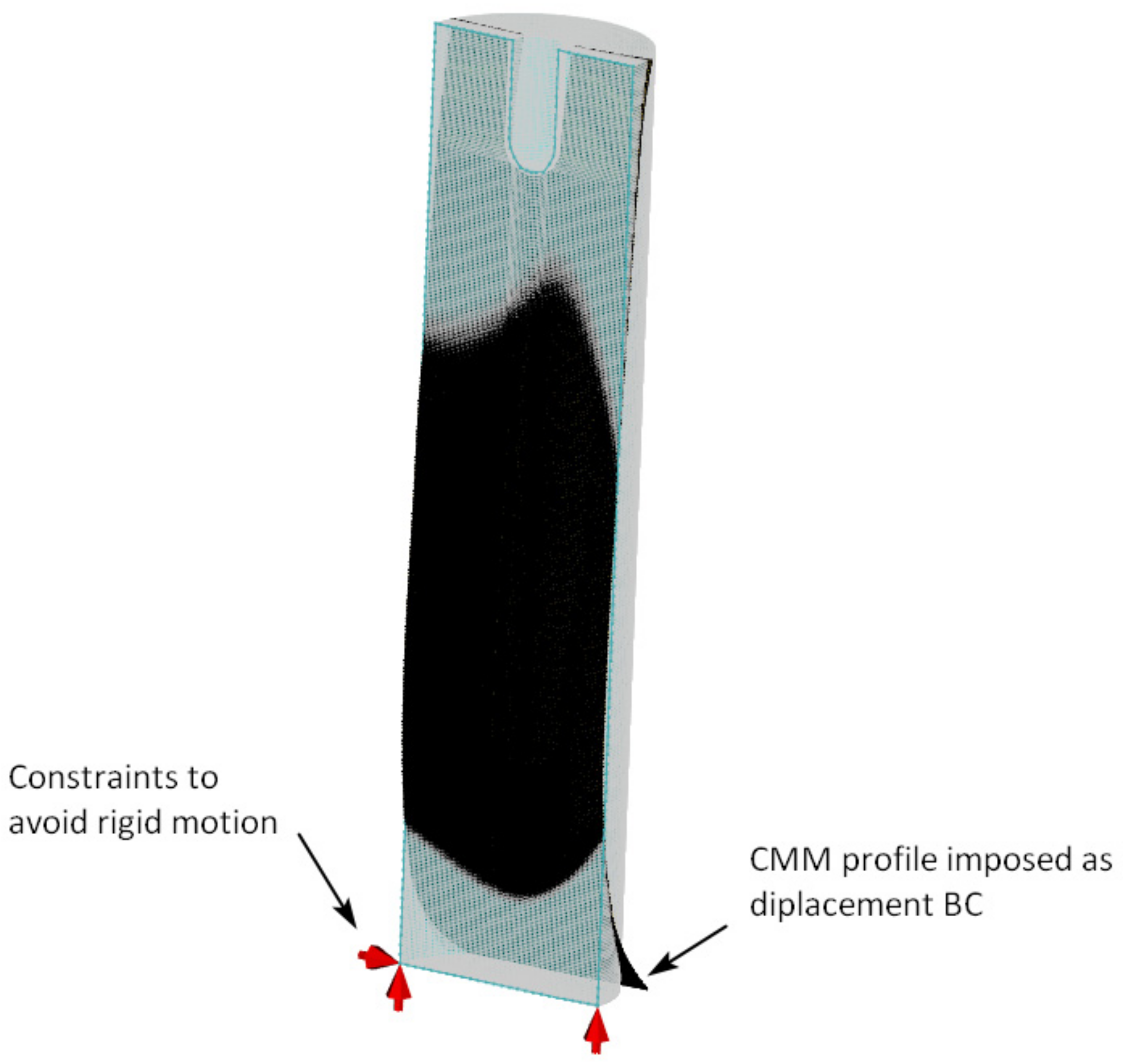
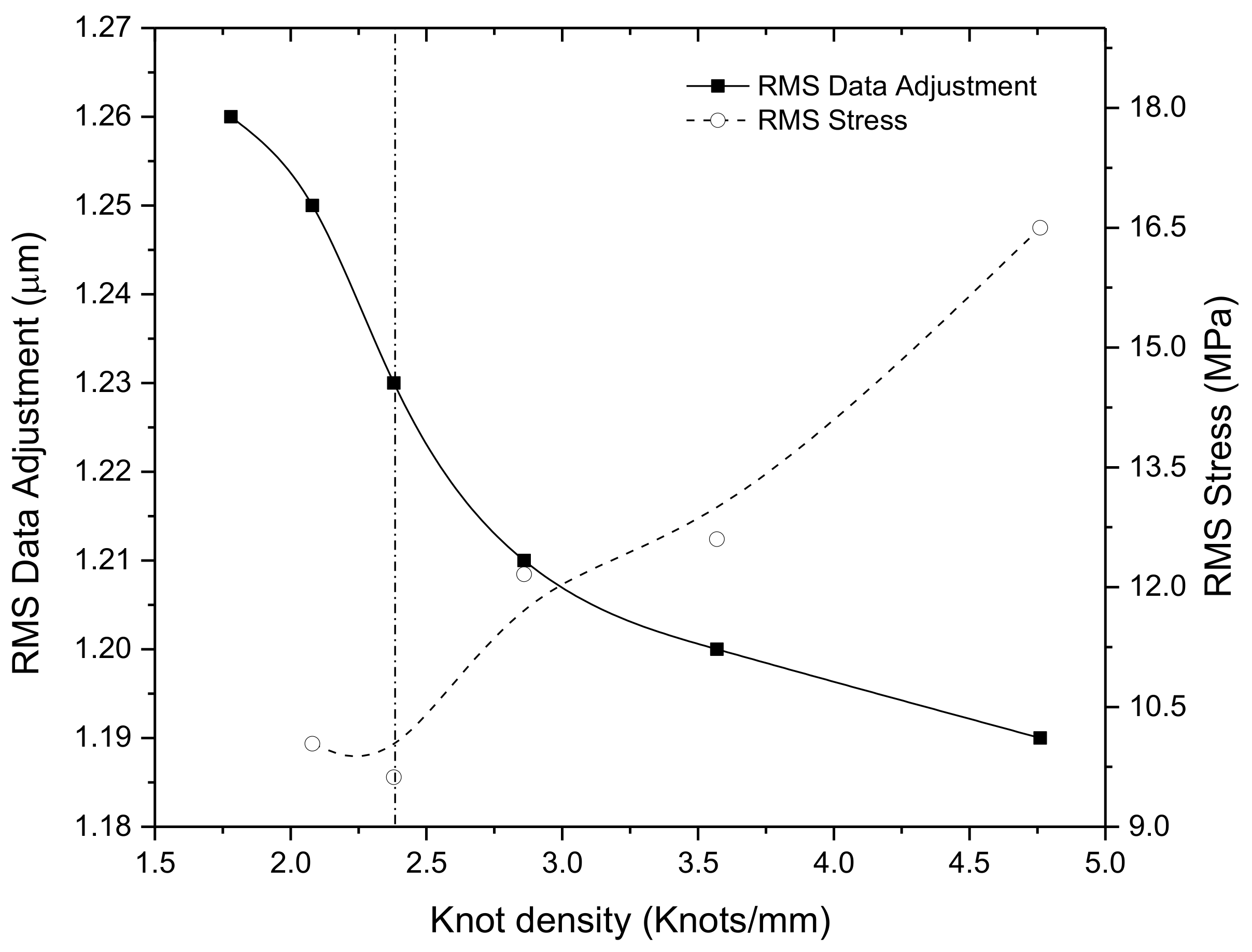
Heat treatment was carried out following the standard Jominy test [24], 100 mm long and 25 mm in diameter AISI 304L samples were maintained at 930 °C for 30 min, followed by fast cooling by waterjet. Samples were instrumented with 3 K-type thermocouples at positions T1, T2, and T3 shown in Figure 1a. Data was acquired using an Omega® data acquisition system OMB-DAQ-2416 (Omega Engineering Inc., Norwalk, CT, USA) and Measurement Computing® software DASYLab 12 (National Instruments Corporation, Austin, TX, USA) for data conditioning and writing. Obtained temperature measurements were used to validate the FEM model thermal accuracy.

Heat treatment simulations were performed using the commercial software package Deform 3D 11.2^® (Scientific Forming Technologies Corporation, Columbus, OH, USA) which is capable to solve coupled problems simultaneously, which included heat transfer phenomena and thermal expansion. Due to the nature of the 304L stainless steel, no phase transformations were considered. A temperature-dependent HTC shown in Figure 3 was added as a boundary condition on the bottom surface. For the above, temperature-dependent properties were employed (Figures 4 and 5).

Symmetry allows to simplify geometry, just a 90° section of the sample were modeled (Figure 1b), enabling a higher number of elements (C3D8 type) in the simulation software. The employed mesh was obtained by its size refinement during successive simulations until the lower average global uncertainty $\left({\overline{\partial \sigma }}_{\left(j\right)}\right)$ was reached, which is the root mean square (RMS) of the normal stress computed in surface nodes according to Equation (1) [25]:

$${\overline{\partial \sigma }}_{\left(j\right)}=\sqrt{\frac{1}{n}{\displaystyle \sum }_{i=1}^n\partial {\sigma }_{\left(i,j\right)}{}^2}$$

(1)

where, $\left(\partial {\sigma }_{\left(i,j\right)}\right)$ is the calculated nodal uncertainty in node (i) and determined refinement mesh grade (j) (ranges defined as j = 1 [1–2 mm], j = 2 [0.7–1.7 mm], j = 3 [0.5–1.7 mm], and j = 4 [0.3–1.7 mm]) with respect to previous, coarser, according to Equation (2) [25]:

$$\partial {\sigma }_{\left(i,j\right)}=\frac{1}{\sqrt{2}}\left|\sigma \left(i,j\right)-\sigma \left(i,j_{-1}\right)\right|$$

(2)

Finally, the selected mesh has elements ranging from 0.3 to 1.7 mm in size (Figure 1b), according to the refinement sequence shown in Figure 2.

The top surface and the cylindrical wall are exposed to natural convection, whereas the bottom surface undergoes forced convection cooling due to the effect of the waterjet. In both cases global time-dependent HTC was used (Figure 3). Values have been calculated using lumped-heat-capacity and inverse method by Narazaki, Sugianto and coworkers [16,17].

In order to assess the effect of effect of HTC variations in the sensitivity of the FEM model residual stress prediction under different cooling conditions, several HTC variations were tested. Such altered coefficients correspond to the original value [16] ±10 kW/m² K and ±100 °C offset, generating an overall of 8 shifted HTCs as shown in Figure 4.

Temperature-dependent mechanical and thermo–physical properties, shown in Figure 5 and Figure 6 respectively, were obtained from literature or calculated through commercial software JMat Pro 9.0^® (Sente Software, Surrey, UK). Atomic emission spectroscopy (AES) was used to obtain the samples chemical composition shown in

Table 1. AISI 304L chemical composition.

Composition	C	Mn	P	S	Si	Ni	Cr
Nominal	0.03	2.0	0.045	0.030	0.75	8.0–12.0	18.0–20.0
Experimental	0.038	1.54	0.027	0.025	0.219	8.0	18.2

and compared to the AISI standard.

2.2. Contour Method

After cooling, specimens were cut using the wire EDM technique, employing an Agie Charmiles Cut 100^® machine using bronze wire of 0.1 mm in diameter and 1 mm per minute cutting speed. Rigid fixation arrangement was necessary to avoid artifacts [22,23,30], in addition, the trajectory of cut started from high stressed edge reducing the plastic deformation effects [31,32,33]. Precautionary measurements were taken to guarantee cutting plane stability as: thermal equilibria between sample and surroundings prior to cutting, usage of sacrificial material [34] to ensure conductivity between cutting sides avoiding transient current effects [35], fixtured set-up can be seen on Figure 7.

Once cut, the surface profile was measured using a Zeiss Eclipse CMM machine fitted with a Renishaw TP8 touch trigger probe (Carl Zeiss AG, Oberkochen, Germany) equipped with an Opto NCDT 2300^® laser scanner (Micro-Epsilon Messtechnik GmbH & Co. KG, Ortenburg, Germany) acquiring a measurement density of approximately 3000 readings per square millimeter. As first data treatment, clouds were cleaned of out-of-boundary points and slight artifacts by means of a Matlab^® R2017a (MathWorks, Natick, Massachussets, USA) tool “CM_Clean” developed by Johnson for his thesis dissertation [36], then both clouds were averaged in a regular spaced grid of around 500,000 points (Figure 8) using pyCM, a Python routine developed by Roy [37].

A surface was fitted to the averaged cloud using second grade spline functions and several points spacing (knots density) with a characteristic RMS value. The fitted surface was then imposed as displacement boundary condition over the nodes in FEM model using Abaqus^® (Abaqus 6.13. Dassault Systemes, France) (Figure 9). The mesh in this model has C3D8 elements of 0.3–1.5 mm in size. Only one plane of symmetry was used to impose the CMM measurements because of the non-symmetric profile obtained.

As mentioned earlier, several Abaqus simulations were carried out using different knots density (also called fitting level). Following Prime’s method [25], the result with the smallest variation in both RMS nodal stress and in RMS data adjustment was selected as the best fitting, as shown in Figure 10.

3. Results

3.1. Quenching Model Thermal Validation

The FEM quenching model was validated in its thermal accuracy by comparing simulated and experimental cooling curves. This is shown in Figure 11. It can be seen that there is a good agreement between the temperature values experimentally measured and those calculated in DEFORM 3D FEM model for all three thermocouple positions.

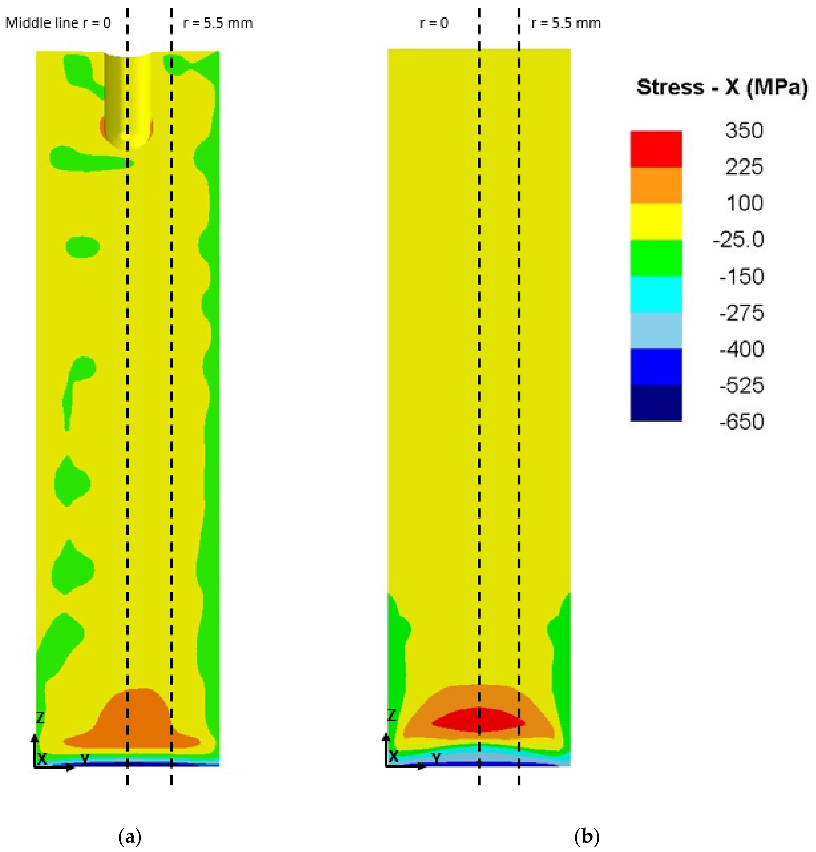
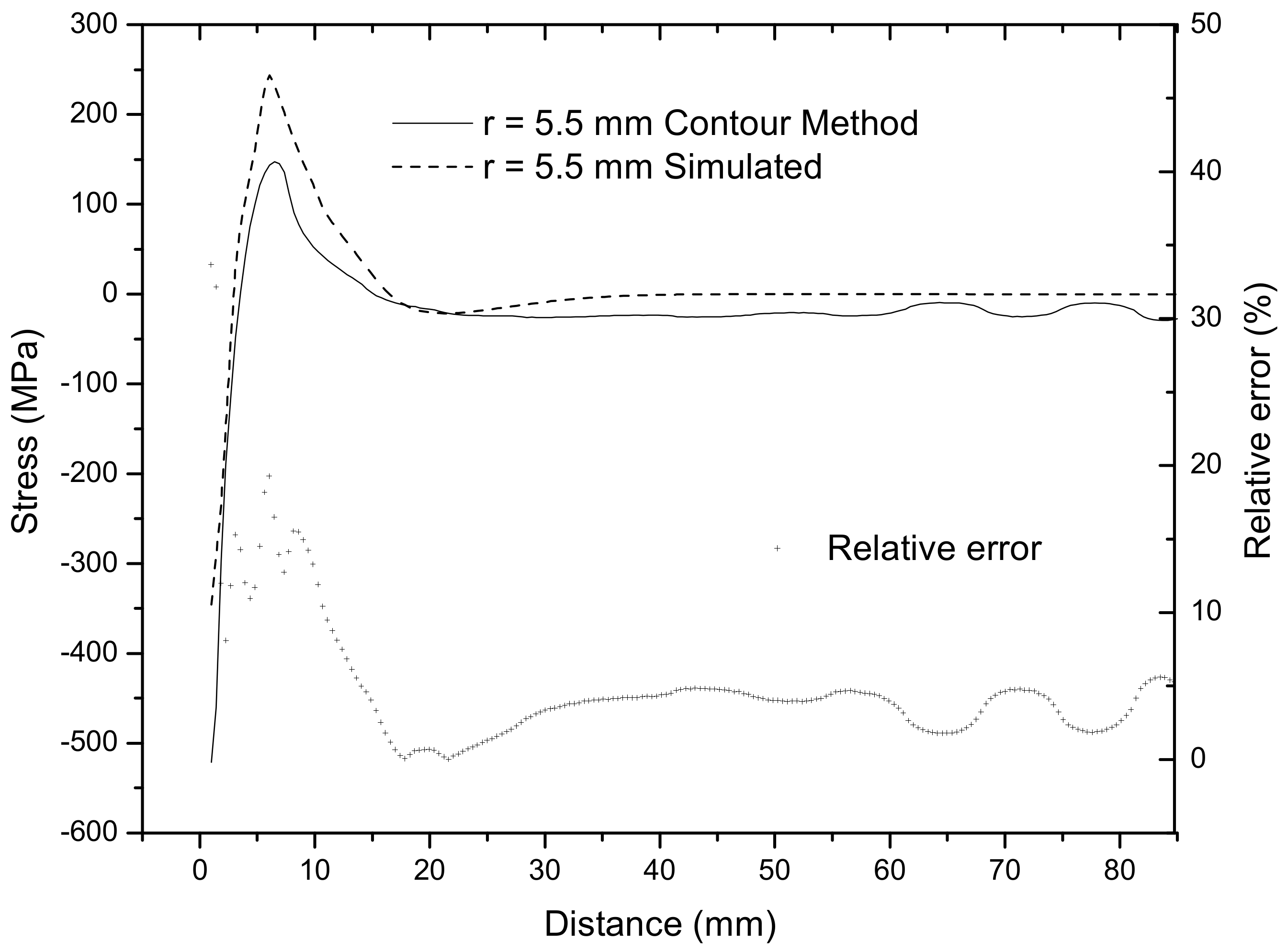
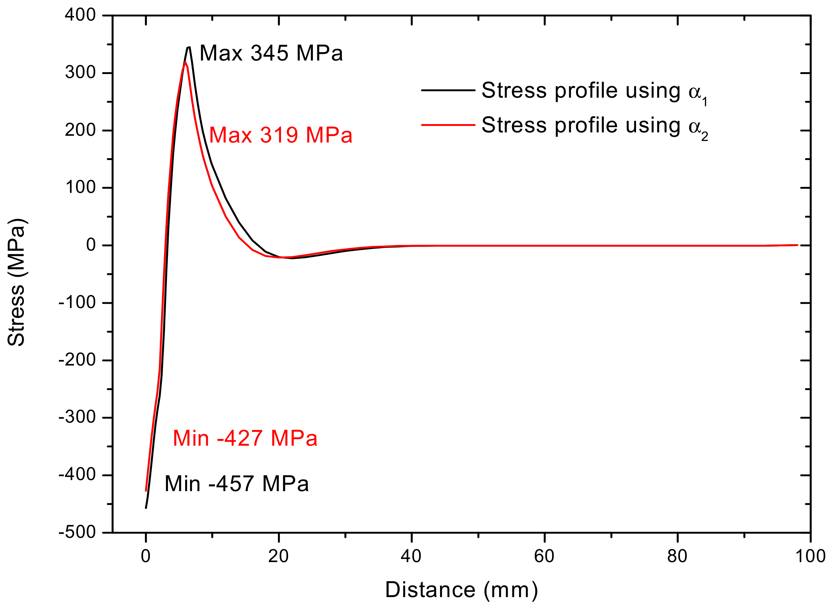
3.2. Contour Method and Modeled Stress Profiles

Results of heat treatment model and contour method measurements from Section 2.1. are both presented in Figure 12, showing the residual stress normal to the cut surface. The measured residual stresses by CM (Figure 12a) show a compressive zone from the end of the quenched bar extending to approximately 2 mm. This is followed by a tensile stress zone extending to approximately 10 mm deep with a maximum value at around 7 mm from the quenched end. The FEM model calculated residual stress profile (Figure 12b) displays a fair coincidence with the CM results, both in stress values and spatial distribution. There are some differences, particularly in the symmetry of the residual stress map along the y direction. This is related to how the FEM model was calculated, with a symmetrical HTC boundary condition imposed on the cylinder lateral surface. It can also be seen that although the measured sample had a bored hole on the top surface, it did not affect the residual stress field since it was far from the quenched area, where the stresses were near zero.

For the sake of a better comparison and taking into account the sample geometry, stress profiles along the center line on the cut plane (y = 12.5 mm) will be referred as r = 0 mm and at y = 18 mm, will be identified as r = 5.5 mm in both results are presented in Figure 13 and Figure 14. Figure 13 shows that the residual stress maximum position is accurately calculated by the FEM model. However, the maximum tensile residual stress magnitude is overestimated by approximately 150 MPa (approximately 20%). Interestingly, the difference between the calculated and measured maximum compressive residual stress is underestimated by approximately 150 MPa as well. As can be seen, the overall error calculated as root mean square error (RMSE) is 41.15 MPa for the center line. Although the error can be seen as relatively high at 20% at the maximum residual stress peak, it quickly goes down to stay at approximately 5%. The position from the quenched end of said maximum residual stress peak is adequately calculated.

Figure 14 shows a similar plot for a linear stress profile calculated at r = 5.5 mm, displaying a similar fitting where the residual stress maxima are in corresponding positions, but the magnitude is overestimated by approximately 100 MPa (15%). The RMSE is slightly lower than the one calculated for the center line at 33.84 MPa.

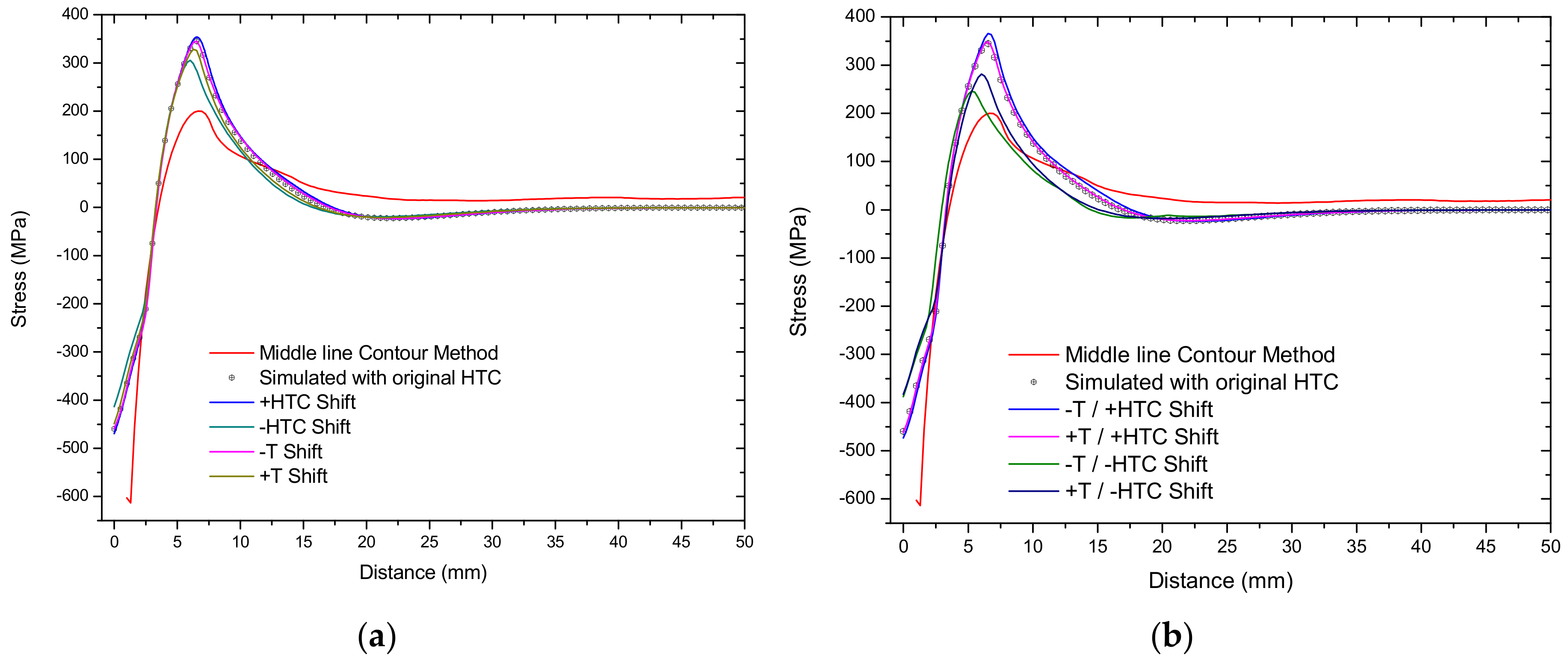
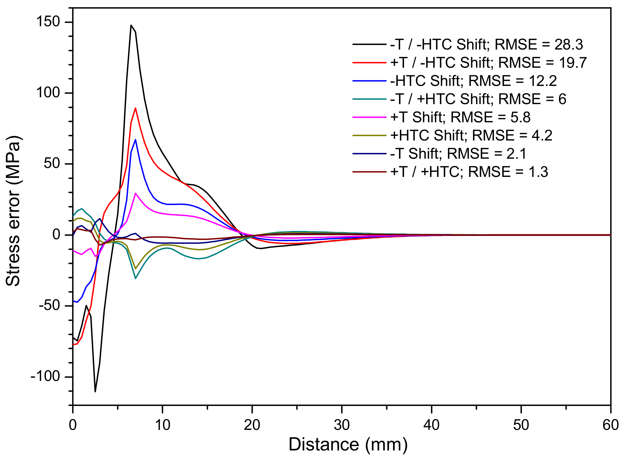
3.3. Parametric Analysis of HTC Variation on Residual Stress Profiles

Hypothetical heat transfer coefficients were introduced to heat treatment model, calculated residual stress profiles and original HTC model results are compared in Figure 15a,b, alongside to its characteristic error in Figure 16.

In Figure 15a, the effect of the hypothetical HTCs (previously presented in Figure 4a) is shown. It can be seen that increasing the heat extraction rate by using an HTC with higher values (+HTC line) has almost no effect in the residual stress profile. Both the magnitude and position of the maximum tensile and compressive residual stresses appear almost unchanged. This also appears to be the case for an HTC shifted to higher (+T line) and lower (−T line) temperatures. Decreasing the HTC, on the other hand, has a more significant effect in both the magnitude and position of the residual stress peak (−HTC line). Using this reduced HTC, however, shifts the maximum tensile residual stress position and decreases the simulated maxima of tensile and compressive residual stresses. The maximum compressive residual stress was not significantly modified in any of the four hypothetical HTC cases.

The combined effect of using a reduced and shifted HTC in the residual stress profile is shown in Figure 15b. It can be seen that an increased HTC does not change the residual stress profile when coupled with either a shift to higher (+T/+HTC line) or lower temperatures (−T/+HTC). In comparison, a reduced HTC (coupled with either a positive or negative temperature shift) does have an effect in the residual stress profile, with the maximum tensile stress shifter nearer to the quenched surface and being reduced in magnitude. These changes, however, do not improve the accuracy of the simulated compressive residual stress maximum, which is still underestimated in all cases.

The effects of the hypothetical HTCs in the residual stress profile are summarized in Figure 16. It can be seen that, as discussed previously, an increased HTC has almost no effect in changing the residual profile, while a reduced HTC, coupled with a negative temperature shift has the most important effect in the simulated residual stress profile.

4. Discussion

It can be seen in the results for all the tested HTCs, that the FEM model does not estimate accurately the residual stress maxima and minima, even though the thermal history is properly calculated. A close look at Figure 13 confirms that the main difference between the measured and calculated residual stress profile is not in the tensile and compressive maxima positions from the edge, but in their magnitude. Interestingly, the maximum tensile residual stress value is overestimated by FEM model by approximately 150 MPa (around 20%), while the maximum compressive stress value is underestimated by the same amount. This is a relatively high magnitude and it may limit the applicability of this kind of models in quenching processes.

In this particular case, thermal-dependent thermophysical properties and expansion were used and no phase transformation was considered. Additionally, the HTC used was previously validated using the inverse method in this geometry [16,17]. Using these properties and boundary conditions, plots such as the ones presented in Figure 11 (thermal validation) and Figure 12 (simulated full-section residual stress profile contours) may lead to an erroneous validation of the FEM model, which needs to be properly assessed using residual stress line profile comparisons. The differences between the simulated and measured residual stress profiles appear unrelated to the thermal accuracy of the model, as shown by the results using several HTC values. Reducing the HTC values does not lead to a significantly lowered maximum residual stress. Additionally, an increased HTC does not, in turn, increase the maximum values for the tensile and compressive residual stresses.

The previous statements lead to question where the difference between measured and simulated residual stress profile is stemming from. Since 304L steel remains austenitic in the quenching range, and no important changes in their thermophysical properties are induced by quenching, the difference should be arising from the material properties themselves. As stated before, 304L steel is not expected to undergo phase transformation during quenching and therefore residual stresses are exclusively thermally generated. As a result of this, it was expected that a more severe quench, as enforced by an increased HTC, should have an effect in the residual stress profile. As shown in Figure 15 and Figure 16, this was not the case. As a result of this, it was decided to explore if the fit between the measured and simulated residual stresses could be improved by using a different thermal expansion coefficient. In order to assess this effect, a new simulation with a thermal expansion coefficient corresponding to a 316 stainless steel was carried out. The thermal expansion coefficient was 1.9 × 10⁻⁵ K⁻¹ for the 304L steel (previously shown in Figure 6c) while the 316 stainless steel thermal expansion coefficient was 1.7 × 10⁻⁵ K⁻¹ [28]. The residual stress profile along the sample central line is presented in Figure 17. It can be seen that using a different thermal expansion coefficient does not have an important effect in the tensile residual stress maximum, rather displacing the position from the quenched end.

Since the simulated residual stress maxima is not affected by varying the HTC or the thermal expansion coefficient, the difference with the CM measured maxima is probably related to plasticity effects. One possibility may be martensite formation. Following the equation proposed by Shen [38] and revisited by Sun [39] (Equation (3)), it is possible to evaluate the possibility of martensite formation versus twinning generation in stainless steels based on the stacking fault energy (SFE) calculated from the steel chemical composition.

$${\gamma }_{SFE}^{RT}\left(\frac{mJ}{m^2}\right)=-53+6.5\%Ni+0.7\%Cr+3.2\%Mn+9.3\%Mo$$

(3)

Following Equation (3), the SFE for the stainless steel quenched in this study is 19.32 mJ m⁻². According to Shen [38], twinning is more favored when the SFE is above 18 mJ m⁻², whereas martensite formation is more likely to occur when the SFE is below 18 mJ m⁻². It can be seen that for this particular steel composition, twinning is more favored than martensite formation. This was further analyzed by observing the microstructure at the maximum tensile residual stress position. The microstructure is shown in Figure 18. The microstructure is fully austenitic, with several twinned austenite grains.

From Figure 18, it is evident that the quenched sample underwent plastic deformation through twinning. This could explain the discrepancy between the calculated and measured residual stress tensile maximum. The FEM model was set to calculate the final stress state for the quenched sample, including both elastic and plastic deformation. The contour method, on the other hand, by definition can only measure elastic relaxation. The FEM model is then overestimating the maximum tensile residual stress because it is not limited to calculate the elastic stress only. In fact, the 304L stainless steel yield stress is 215 MPa, which is just above the 200 MPa tensile residual stress maximum measured by the contour method. Previous papers [2,6] comparing measured and FEM calculated residual stresses in quenched stainless steel have shown that the tensile residual stress maximum is consistently overestimated by the FEM model.

The underestimation of the compressive residual stress maximum is most likely related to the shortcomings of the FEM model, in particular during the calculation of the residual stress at the highest cooling rate near the quenched end. In a previous study by Hossain [2], the occurrence of these high compressive residual stresses is thought to be related to the high strain rate found in the quenched end which may increase the stainless steel yield stress. As previously shown in Figure 5b, the flow stress used in the model presented is temperature-dependent but not strain-rate-dependent.

5. Conclusions

Current FEM models capable of simulating quenching are readily available, however thermal history fit must not be used as the sole parameter to validate the model especially in terms of residual stress profiles. The Deform 3D FEM model presented is capable of accurately representing the thermal story throughout the quenching process of a 304L stainless steel. Residual stresses maximum (both tensile and compressive) positions from the quenched end are in good agreement with the ones measured by contour method. Tensile residual stress maximum magnitude is overestimated, while the maximum compressive residual stress is underestimated by approximately the same amount (20%). The differences in residual stress magnitude could not be corrected by modifying the HTC in the FEM model nor with using a different thermal expansion coefficient. Residual stresses in this material should exclusively be thermally generated. However, following stacking fault energy calculations and metallography of the quenched area, the sample underwent plastic deformation through twining. This mechanism needs to be taken into account in future stainless steel quenching models.

References

1. Wither, P.J. Residual stress and its role in failure. Rep. Prog. Phys. 2007, 70, 2211–2264. [Google Scholar] [CrossRef] [Green Version]
2. Hossain, S.; Daymond, M.R.; Truman, C.E.; Smith, D.J. Prediction and measurement of residual stresses in quenched stainless-steel spheres. Mater. Sci. Eng. A 2004, 373, 339–349. [Google Scholar] [CrossRef]
3. Prime, M.B. Residual Stresses Measured in Quenched HLSA-100 Steel plate. In Proceedings of the 2005 SEM Annual Conference and Exposition on Experimental and Applied Mechanics, Portland, OR, USA, 7–9 June 2005; Volume 836, pp. 1–8. [Google Scholar]
4. Turski, M.; Edwards, L. Residual stress measurement of a 316l stainless steel bead-on-plate specimen utilising the contour method. Int. J. Press. Vessel. Pip. 2009, 86, 126–131. [Google Scholar] [CrossRef]
5. Schulze, V.; Vöhringer, O.; Macherauch, E. Residual stresses after quenching. In Quenching Theory and Technology; Liscic, B., Tensi, H.M., Canale, L.C.F., Totten, G.E., Eds.; CRC Press: Boca Raton, FL, USA, 2010; p. 725. ISBN 978-0-8493-9279-5. [Google Scholar]
6. Hosseinzadeh, F.; Hossain, S.; Truman, C.E.; Smith, D.J. Measurement and Prediction of Residual Stresses in Quenched Stainless Steel Components. Exp. Mech. 2014, 54, 1151–1162. [Google Scholar] [CrossRef]
7. Hakan, G.C.; Erman, T.A. Numerical and experimental analysis of quench induced stresses and microstructures. J. Mech. Behav. Mater. 1998, 9, 237–256. [Google Scholar]
8. Sen, S.; Aksakal, B.; Ozel, A. Transient and residual thermal stresses in quenched cylindrical bodies. Int. J. Mech. Sci. 2000, 42, 2013–2029. [Google Scholar] [CrossRef]
9. Lu, Y. Heat Transfer, Hardenability and Steel Phase Transformations during Gas Quenching; Worcester Polytechnic Institute: Worcester, MA, USA, 2016. [Google Scholar]
10. Lu, Y.; Sisson, R.D.; Rong, Y.K.; Macsari, J. Critical heat transfer coefficient test for gas quench steel hardenability. In Proceedings of the 28th ASM Heat Treating Society Conference, Detroit, MI, USA, 20–22 October 2015; pp. 484–488. [Google Scholar]
11. Evcil, G.E.; Mustak, O.; Simsir, C. Simulation of through-hardening of SAE 52100 steel bearings—Part II: Validation at industrial scale. Materwiss. Werksttech. 2016, 47, 746–754. [Google Scholar] [CrossRef]
12. Buczek, A.; Telejko, T. Investigation of heat transfer coefficient during quenching in various cooling agents. Int. J. Heat Fluid Flow 2013, 44, 358–364. [Google Scholar] [CrossRef]
13. Le Masson, P.; Loulou, T.; Artioukhine, E. Numerical estimations of a two-dimensional convection heat transfer coefficient during a metallurgical “Jominy end-quench” test. Int. J. Therm. Sci. 2002, 41, 517–527. [Google Scholar] [CrossRef]
14. Liščić, B.; Filetin, T. Measurement of quenching intensity, calculation of heat transfer coefficient and global database of liquid quenchants. Mater. Eng. 2012, 19, 52–63. [Google Scholar]
15. Le Masson, P.; Loulou, T.; Artioukhine, E. Estimations of a 2D convection heat transfer coefficient during a metallurgical “Jominy end-quench” test: Comparison between two methods and experimental validation. Inverse Probl. Sci. Eng. 2004, 12, 595–617. [Google Scholar] [CrossRef]
16. Narazaki, M.; Kogawara, M.; Shirayori, A.; Fuchizawa, S. Evaluation of heat transfer coefficient in Jominy end-quench test. In Proceedings of the Fourth International Conference on Quenching and the Control of Distortion, Beijing, China, 20–26 May 2003. [Google Scholar]
17. Sugianto, A.; Narazaki, M. Validity of heat transfer coefficient based on cooling time, cooling rate, and heat flux on Jominy end quench test. In Proceedings of the STEEL: Recent Developments in Steel Processing. AIST Steel Properties and Applications Conference, Detroit, MI, USA, 16–20 September 2007; pp. 171–180. [Google Scholar]
18. Gür, C.H.; Şimşir, C. Simulation of Quenching: A Review. Mater. Perform. Charact. 2012, 1, 104479. [Google Scholar] [CrossRef]
19. Prime, M.B. Cross seccional mappig of residual rtresses by measuring the surface contour after a cut. J. Eng. Mater. Technol. 2001, 836, 162–168. [Google Scholar] [CrossRef] [Green Version]
20. Moat, R.J.; Ooi, S.; Shirzadi, A.A.; Dai, H.; Mark, A.F.; Bhadeshia, H.K.D.H.; Withers, P.J. Residual stress control of multipass welds using low transformation temperature fillers. Mater. Sci. Technol. 2018, 34, 519–528. [Google Scholar] [CrossRef]
21. Bueckner, H.F. The propagation of cracks and the energy of elastic deformation. Trans. Am. Soc. Mech. Eng. 1958, 80, 1225–1230. [Google Scholar]
22. Bouchard, P.J.; Ledgard, P.; Hiller, S.; Hosseinzadh, F. Making the cut for the contour method. In Proceedings of the 15th International Conference on Experimental Mechanics, Porto, Portugal, 22–27 July 2012. [Google Scholar]
23. Hosseinzadeh, F.; Kowal, J.; Bouchard, P.J. Towards good practice guidelines for the contour method of residual stress measurement. J. Eng. 2014, 2014, 453–468. [Google Scholar] [CrossRef]
24. ASTM A 255 Norm, 2002 “Standard Test Methods for Determining Hardenability of Steel”; ASTM International: West Conshohocken, PA, USA, 2002; pp. 1–26.
25. Prime, M.B.; Sebring, R.J.; Edwards, J.M.; Hughes, D.J.; Webster, P.J. Laser surface-contouring and spline data-smoothing for residual stress measurement. Exp. Mech. 2004, 44, 176–184. [Google Scholar] [CrossRef]
26. Lewis, J.R. Physical Properties of Stainless Steels. In Handbook of Stainless Steels; Peckner, D.I., Bernstain, I.M., Eds.; McGraw-Hill: New York, NY, USA, 1977; ISBN 0-07-049147-X. [Google Scholar]
27. Austenitic Chromium-Nickel Stainless Steels Engineering Properties at Elevated Temperatures; The Nickel Development Insitute: New York, NY, USA, 1978.
28. JMatPro Manual; Sente Software: Surrey, UK, 2016.
29. Bogaard, R.H.; Desai, P.D.; Li, H.H.; Ho, C.Y. Thermophysical properties of stainless steels. Thermochim. Acta 1993, 218, 373–393. [Google Scholar] [CrossRef]
30. Prime, M.B. The contour method: Capabilities, limitations, and recent advances. In Proceedings of the 4th Residual Stress Summit, Lake Tahoe, CA, USA, 26–29 September 2010; p. 470. [Google Scholar]
31. Traoré, Y.; Hosseinzadeh, F.; Bouchard, P.J. Plasticity in the contour method of residual stress measurement. Adv. Mater. Res. 2014, 996, 337–342. [Google Scholar] [CrossRef] [Green Version]
32. Hosseinzadeh, F.; Yeli, T.; Bouchard, P.J.; Muránsky, O. Mitigating cutting-induced plasticity in the contour method. Part 1: Experimental. Int. J. Solids Struct. 2016, 94, 247–253. [Google Scholar] [CrossRef]
33. Sun, Y.L.; Roy, M.J.; Vasileiou, A.N.; Smith, M.C.; Francis, J.A.; Hosseinzadeh, F. Evaluation of errors associated with cutting-induced plasticity in residual stress measurements using the contour method. Exp. Mech. 2017, 57, 719–734. [Google Scholar] [CrossRef] [PubMed] [Green Version]
34. Flack, D.; Medina-Juarez, I.; (The Open University). Personal communication, 2017.
35. Ahmad, B.; Fitzpatrick, M.E. Minimization and mitigation of wire EDM cutting errors in the application of the contour method of residual stress measurement. Metall. Mater. Trans. A 2015, 47, 301–313. [Google Scholar] [CrossRef]
36. Johnson, G. Residual Stress Measurements Using the Contour Method; University of Manchester: Manchester, UK, 2008. [Google Scholar]
37. Roy, M. pyCM Software. Available online: https://github.com/majroy/pyCM (accessed on 30 June 2019).
38. Shen, Y.F.; Li, X.X.; Sun, X.; Wang, Y.D.; Zuo, L. Twinning and martensite in a 304 austenitic stainless steel. Mater. Sci. Eng. A 2012, 552, 514–522. [Google Scholar] [CrossRef]
39. Sun, G.; Du, L.; Hu, J.; Zhang, B.; Misra, R.D.K. On the influence of deformation mechanism during cold and warm rolling on annealing behavior of a 304 stainless steel. Mater. Sci. Eng. A 2019, 746, 341–355. [Google Scholar] [CrossRef]
Figure 1. (a) Real sample geometry and thermocouples position, dimensions in mm; (b) Simplified 90° meshed geometry.
Metals 09 01308 g001
Figure 2. Mesh refinement for Deform 3D simulation, j stands for refinement mesh grade, following the ranges shown in the figure itself.
Metals 09 01308 g002
Figure 3. Calculated heat transfer coefficient (HTC) in Jominy test by Narazaqui.
Metals 09 01308 g003
Figure 4. Hypothetical and original HTC (a) Temperature and HTC shifts; (b) Combined shifts.
Metals 09 01308 g004
Figure 5. Mechanical properties (a) Young´s modulus [26] and Poisson´s ratio [27]; (b) Flow stress [28].
Metals 09 01308 g005
Figure 6. Thermo–physical properties (a) Heat capacity [27,29]; (b) Conductivity [26]; (c) Linear thermal expansion [29].
Metals 09 01308 g006
Figure 7. Fixture system and sacrificial material on sample.
Metals 09 01308 g007
Figure 8. Two data sets (orange and yellow) averaged in a single cloud (blue).
Metals 09 01308 g008
Figure 9. Fitted surface imposed as a boundary condition on contour method model.
Metals 09 01308 g009
Figure 10. Selected knot density in data fitting.
Metals 09 01308 g010
Figure 11. Experimental and simulated cooling curves validating the FEM thermal response model.
Metals 09 01308 g011
Figure 12. Normal-to-surface residual stress plot obtained by (a) Contour method; (b) Deform 3D FEM simulation.
Metals 09 01308 g012
Figure 13. Normal residual stress comparison between the CM measurements and FEM model at middle line (r = 0 mm) and its relative error.
Metals 09 01308 g013
Figure 14. Normal residual stress comparison between the CM measurements and FEM model at r = 0 mm and its relative error.
Metals 09 01308 g014
Figure 15. Simulated stress profiles on middle line using hypothetical HTC values: (a) ±T and ±HTC; (b) ±T/±HTC combinations.
Metals 09 01308 g015
Figure 16. Residuals relative to original HTC simulated stress profile.
Metals 09 01308 g016
Figure 17. Residual stress profile along the sample central line for the 304L (α1) and 316 (α2) thermal expansion coefficients.
Metals 09 01308 g017
Figure 18. Microstructure of the quenched sample at the maximum tensile residual stress zone.
Metals 09 01308 g018