Interlaboratory Measurements of Contiguity in WC-Co Hardmetals

Abstract

The contiguity of a hardmetal is a measure of the proportion of the carbide grain boundaries that are in direct contact with other carbide grain boundaries. Recent analysis of data available in the literature shows a large scatter in results and a significant difference in values measured from scanning electron microscope (SEM) images and from electron backscatter diffraction (EBSD) mapping. An interlaboratory exercise has been carried out with the measurement of a range of WC-Co hardmetal grades. For each grade, SEM images were acquired from both an etched surface and an ion beam polished surface and EBSD maps with two different processing routes. These maps and images were provided to the participants for measurement to eliminate variability from sample preparation and image acquisition. It was shown that measurement of contiguity from EBSD maps is likely to lead to an overestimation of contiguity, largely because EBSD maps do not have the resolution of SEM images to identify small binder phase regions between WC grains. Ion beam polishing combined with backscattered electron imaging was found to provide the best images of the microstructure to underpin a confident measurement of contiguity. However, high resolution SEM images of etched surfaces gave values close to those from ion beam polished samples so it is recommended that, as etching is much more widely available, high-resolution imaging of a lightly etched WC surface should be promoted as the preferred method for measurement of contiguity, in combination with backscattered imaging where possible. Even with good images, variation between operators can give uncertainties of approximately ±10%.

1. Introduction

The contiguity of a hardmetal is a measure of the proportion of the carbide grain boundaries that are in direct contact with other carbide grain boundaries. Contiguity is an important characteristic of the microstructure of hardmetals and is likely to play an important role in the determination of mechanical, electrical and thermal properties through its effect on interface structure. For example, within hardmetal structures, the two main types of interface, WC/WC and WC/Co, have different conductances (thermal and electrical) and contiguity is a parameter which defines their relative contributions to the overall conductivities of materials with different compositions and grain sizes. Equally, these interfaces are key to the extent of load transfer in mechanically deformed materials. Thus contiguity affects the strength and toughness of different hardmetal compositions. It should be defined in terms of grain boundary areas, but in practice measurement is made by a linear intercept method, counting the number of carbide-carbide boundaries, N_WC, and of carbide-binder boundaries, N_Co-WC, and determining the contiguity, C, from the equation

$$C=\frac{2N_{WC}}{2N_{WC}+N_{Co-WC}}.$$

(1)

Details of this derivation and the relationship of contiguity to the other key microstructural parameters are given in [1]. Analysis of data in the literature shows a large degree of scatter in the values of contiguity when plotted against the cobalt volume fraction (Figure 1) [1,2,3,4,5,6]. However, it has been difficult to determine how much of this scatter is a result of real variation (since C will also be a function of WC grain size and the Co binder mean free path) and how much is a result of failure to detect or incorrect identification of the boundaries present because of instrument resolution limitations or etching effects.

The increasing use of EBSD as a technique for microstructural analysis of hardmetals was initially thought to provide an opportunity for accurate and reproducible measurement of contiguity. EBSD can distinguish between different WC grains definitively on the basis of crystallographic orientation rather than subjectively and dependent on avoidance of over- or under-etching. However, the observation of the position and type of boundary is constrained by EBSD operating parameters such as pixel size (resolution) and acquisition times. Comparison of EBSD measurements with those from high-resolution SEM images (Figure 1) shows that, for a given Co volume fraction, Co V_f, the former results are consistently significantly higher than those from SEM images, although this difference is no larger than that between all the SEM image measurements themselves.

To complement a recent National Physical Laboratory, NPL, paper [7] on the metrology of contiguity measurements, an interlaboratory exercise has been carried out in which four different hardmetal grades were imaged in the SEM and by EBSD at NPL. Identical images were then distributed to four laboratories for measurements of contiguity by a manual linear intercept method. Results from the interlab together with specifically detailed analysis of the preparation methods at NPL are summarised in this paper together with recommendations on good measurement practice.

2. Methods

Four WC-Co samples were chosen for measurement that covered a range of binder phase content (6 to 20 wt.%) and linear intercept grain size (0.59–2.75 µm). Details are summarised in

Table 1. Raw Material data for samples examined.

Code	Co wt.% (Nominal)	Co vol.% (Nominal)	Coercivity kA/m	HV30	WC Grain Size—µm
					ECD	LI
					EBSD	EBSD
6SM	5.9	9.9	15.9	1625	0.66	0.59
10M	10.1	16.5	6.4	1125	2.09	2.2
15SM	15.3	24.1	10.3	1250	0.77	0.72
20C	20.2	30.8	4	850	3.32	2.75

, where ECD is equivalent circle diameter and LI is a linear intercept, in both cases measured from EBSD maps [8,9], obtained from the measurement of a minimum of 300 grains.

Images of the microstructures were provided to the participants for manual measurement of the contiguity to eliminate the variability that might be caused by sample preparation; because participants might not necessarily have access to the variety of techniques used in this exercise by NPL.

The samples were polished by conventional mechanical means with the last stage being colloidal silica for 20 min. A final polish was given to each sample in a Hitachi IM4000 (Hitachi, Krefeld, Germany) argon ion mill, using a 3-degree glancing incidence beam and steps of 30 min at each of 6, 3 and 1.5 kV. After imaging in this as-polished condition (see below) the samples were etched with Murakami’s reagent for times estimated by the metallographer to be suitable for each grade.

The images were obtained at NPL using a Zeiss Auriga or Zeiss Supra SEM (Zeiss, Cambridge, UK). Backscattered electron images were acquired with the former (at 10 kV and approximately 10 mm working distance.) and EBSD maps were acquired with a TSL-EDAX Hikari (EDAX, Draper, UT, USA) detector using the latter microscope (at 20 kV, 15 mm working distance and high current from a 120 µm aperture). Secondary electron images of the samples after etching were acquired with the Zeiss Supra SEM (Zeiss, Cambridge, UK).

Four image types were supplied:

• Backscattered Electron Images on ion beam polished samples.
• EBSD maps on ion beam polished samples:

  ◦

  EBSD 1: Orientation coloured (Inverse pole figure (IPF) scale) on a grey scale EBSD pattern quality map after minimal cleaning/re-indexing.

  ◦

  EBSD 2: Orientation coloured (IPF scale) on a black background without cleaning.

• Etched (Murakami’s) samples (secondary electron or backscattered images). Etched after mechanical polishing.

Figure 2 shows examples of each image for the material 10M. Participants were requested to measure from the images using their normal procedure, with the suggestion that a minimum of 200 intercepts were to be measured.

3. Results and Discussion

Measurements of contiguity were returned from four laboratories (including NPL) and for one of these laboratories, two people independently measured the images, giving five sets of data in total. The raw results are shown in

Table 2. Contiguity measurements on all four hardmetal grades from five participants A–E. Blank cells indicate no measurement reported by participants. Outliers (more than 1 standard deviation from the mean indicated by italics).

Backscattered
Code	A	B	C	D	E	Mean	Std. Dev.
6SM	0.63	0.59	0.52	0.6	0.49	0.57	0.06
10M	0.48	0.47	0.43	0.46	0.4	0.45	0.03
15SM	0.51	0.46	0.45	0.46	0.52	0.48	0.03
20C	0.30	0.31	0.27	0.32	0.21	0.28	0.04
EBSD on grey scale (EBSD 1)
Code	A	B	C	D	E	Mean	Std. Dev.
6SM	0.77	0.78	-	0.75	0.81	0.78	0.03
10M	0.60	0.58	0.53	0.55	0.61	0.57	0.03
15SM	0.64	0.67	0.58	0.56	0.75	0.64	0.08
20C	0.48	0.44	0.34	0.36	0.43	0.41	0.06
EBSD on Black (EBSD 2)
Code	A	B	C	D	E	Mean	Std. Dev.
6SM	0.73	0.77	0.6	-	0.75	0.71	0.07
10M	0.57	0.55	-	-	0.58	0.57	0.01
15SM	0.59	0.62	-	-	0.58	0.60	0.02
20C	0.36	0.38	-	-	0.29	0.34	0.05
Etched
Code	A	B	C	D	E	Mean	Std. Dev.
6SM	0.62	0.67	0.41	0.69	0.61	0.60	0.11
10M	0.56	0.5	0.47	0.55	0.49	0.51	0.04
15SM	0.48	0.44	0.33	0.49	0.51	0.45	0.06
20C	0.38	0.36	0.38	0.35	0.44	0.38	0.04

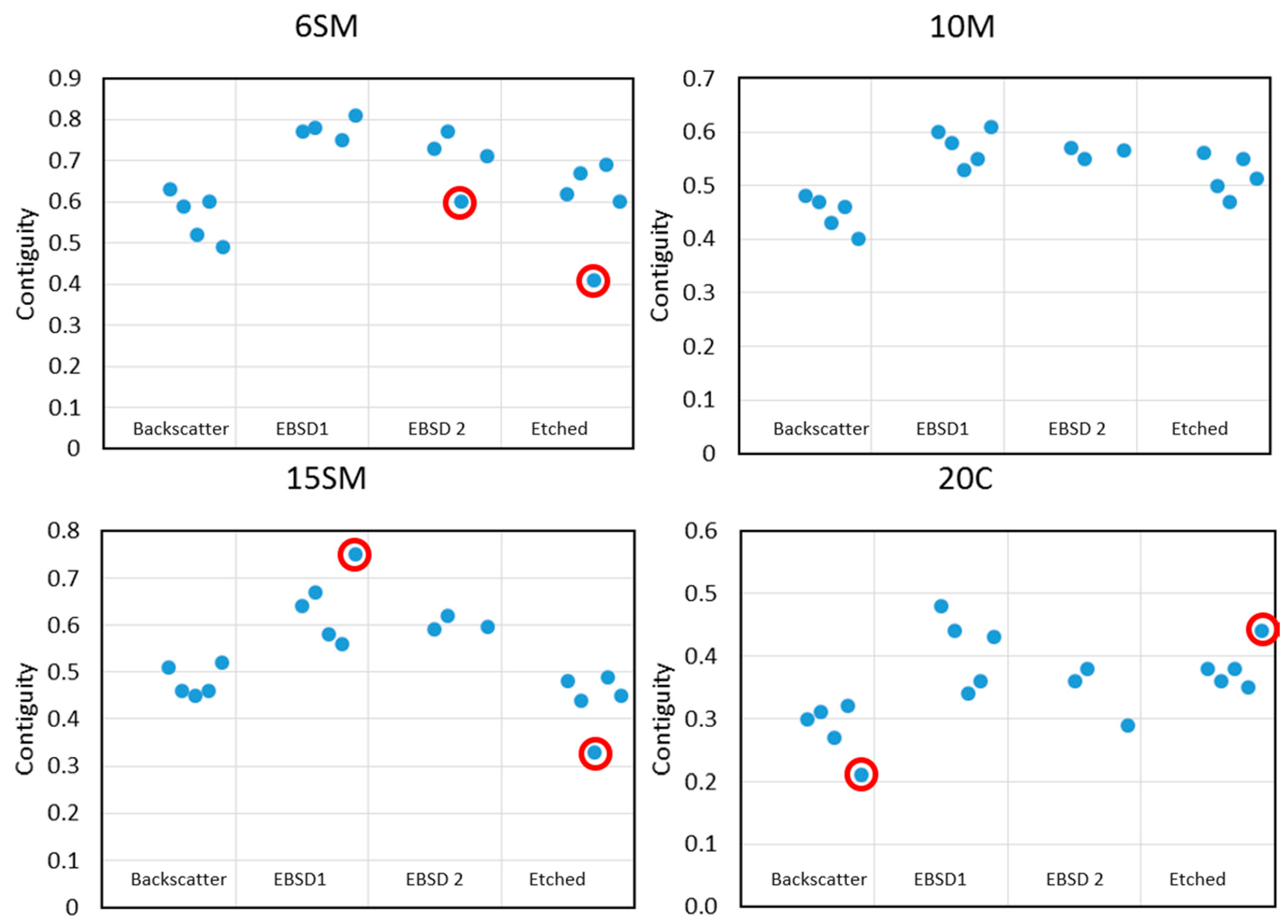
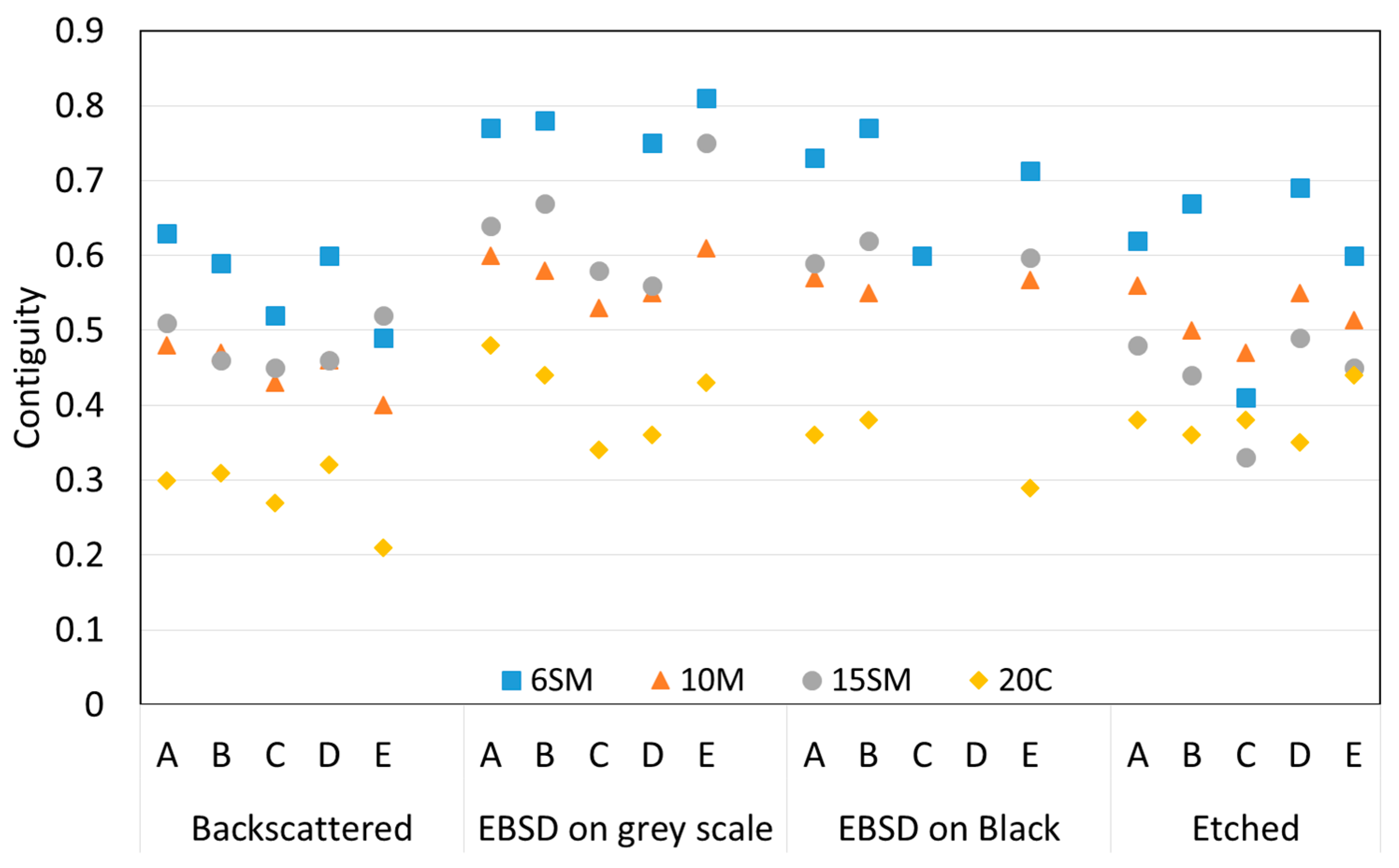
for the five data sets labelled A–E. Figure 3 shows individual sets of data for each grade of material and Figure 4 all these results in one graph.

Figure 3 shows these results as individual sets of data for each grade of material and Figure 4 all the results in one graph. Outliers (differing from the mean by more than one standard deviation) indicated in italics.

It should be noted from Figure 3 that a few data points appear to be significantly different from the cluster of four other measurements from the same image type for a given material. These data points were more than one standard deviation from the mean of the results for that set and are ringed in red. In some of the subsequent analysis, these points have been treated as outliers and excluded from calculations of mean values. Another significant point to note is that the EBSD maps with a black background (EBSD2) were only analysed by three laboratories for three of the four material grades, which could contribute to a reduction in the apparent degree of scatter measured for this map type.

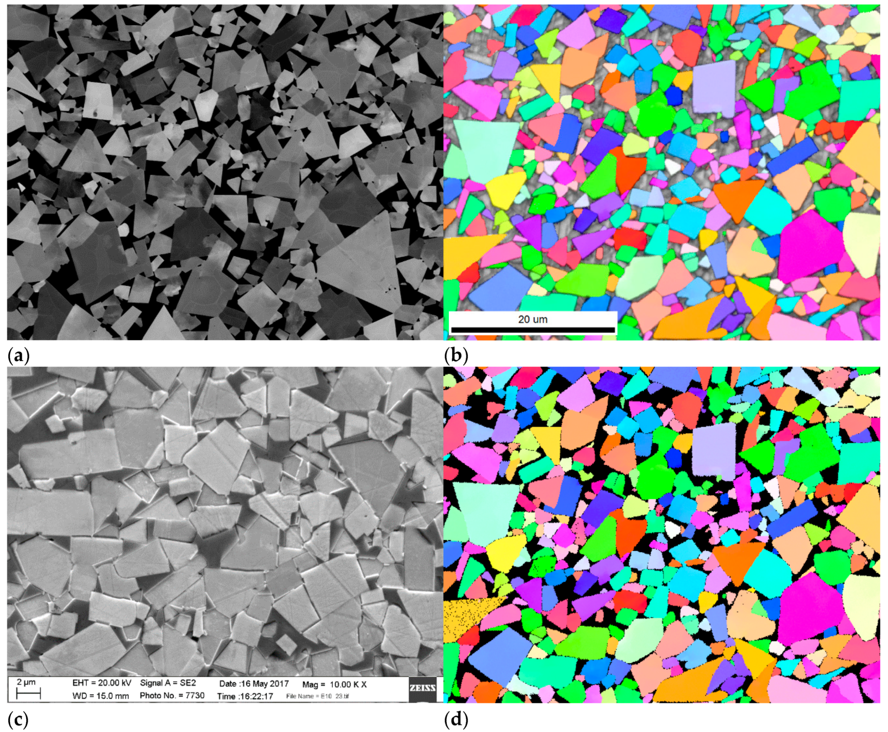
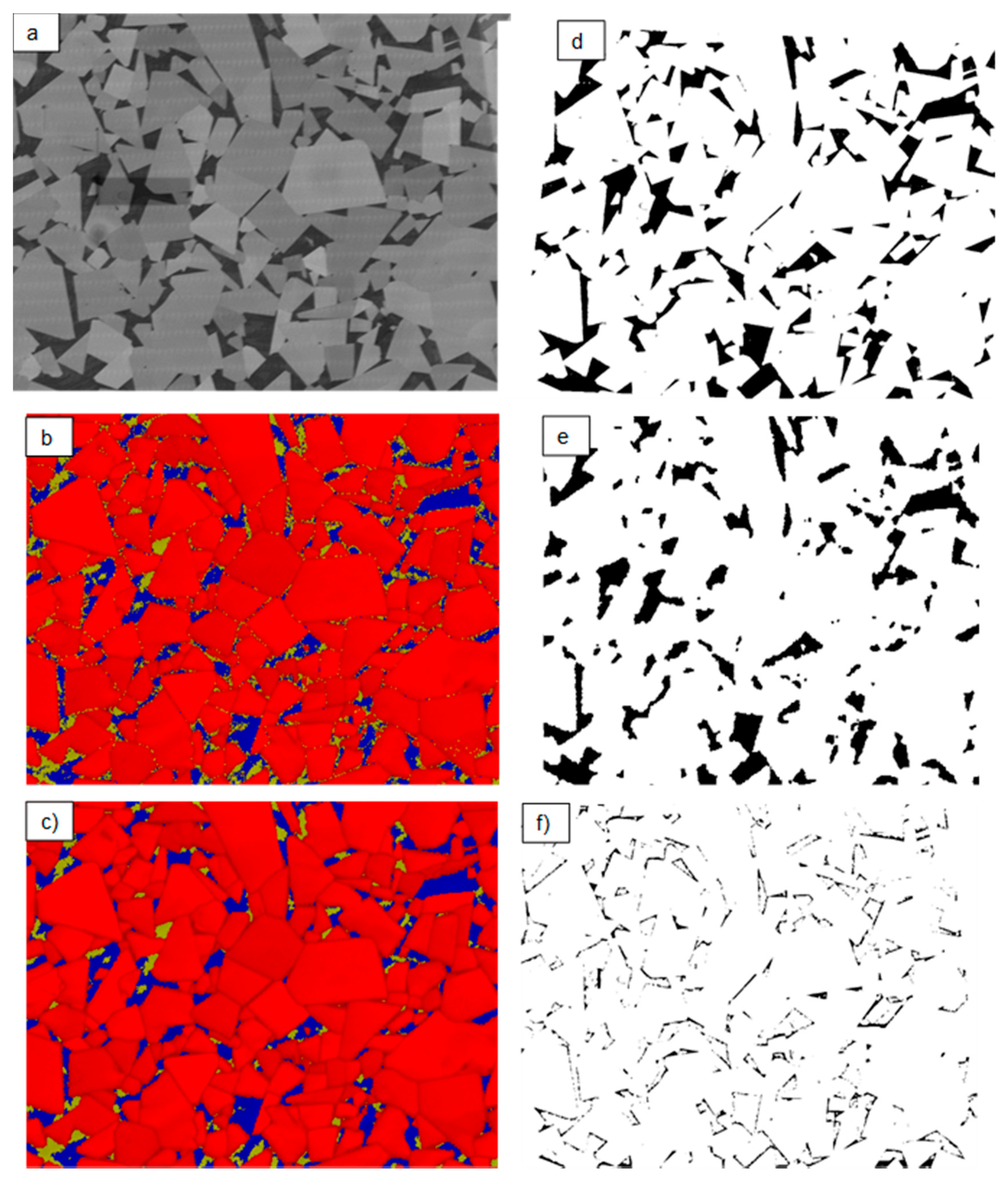
It is instructive that the following discussion has been influenced by earlier work at NPL [7] in which a direct comparison of an EBSD map was made with a backscattered image of the same area. This comparison is shown in Figure 5. The EBSD maps in Figure 5b,c were acquired with a step size of 0.1 µm while the backscatter image (Figure 5a) pixel size is 0.03 µm. This map to image pixel size ratio is similar to that used for the maps and images in the interlaboratory study which were typical for the parameters needed to acquire image or EBSD maps in a realistic timescale. The effective erosion of the Co binder in the EBSD map by the coarser step size is most clearly seen in Figure 5f, obtained by subtraction of a thresholded image of the binder phase in the EBSD map (Figure 5e) from that of the thresholded backscattered image (Figure 5d). The clear identification of the binder phase in the backscatter image and the good contrast between grains that this imaging method produces means that, in the opinion of the authors, this imaging method is likely to give the most accurate representation of the microstructure from which to make measurements of contiguity. For this reason, the results from measurements of these images in this interlab exercise have been used as a baseline value against which the other measurements have been compared.

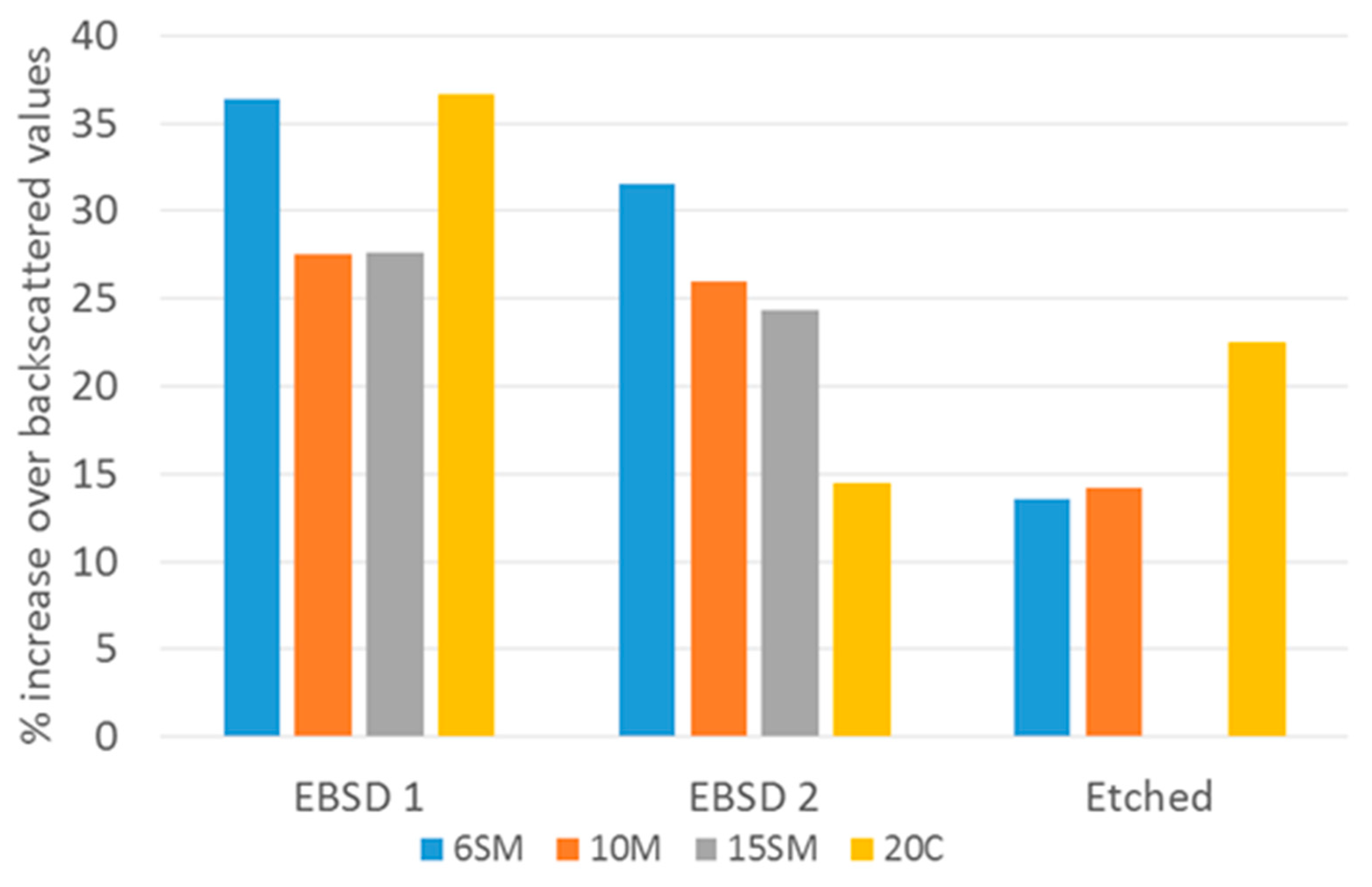
Figure 6 summarises the data in Figure 3 and Figure 4 by plotting the average contiguity for each sample and each measurement technique with error bars showing the range of values measured. It is clear that the backscattered images consistently produced the lowest values of contiguity of any of the four measurement types. Figure 7 shows this trend as a percentage increase above the backscattered value of contiguity; the EBSD maps giving on average 30% higher values for the grey scale background and 25% for the black background, and the etched images about 15% higher (with one exception for 15SM which gave exactly the same average value).

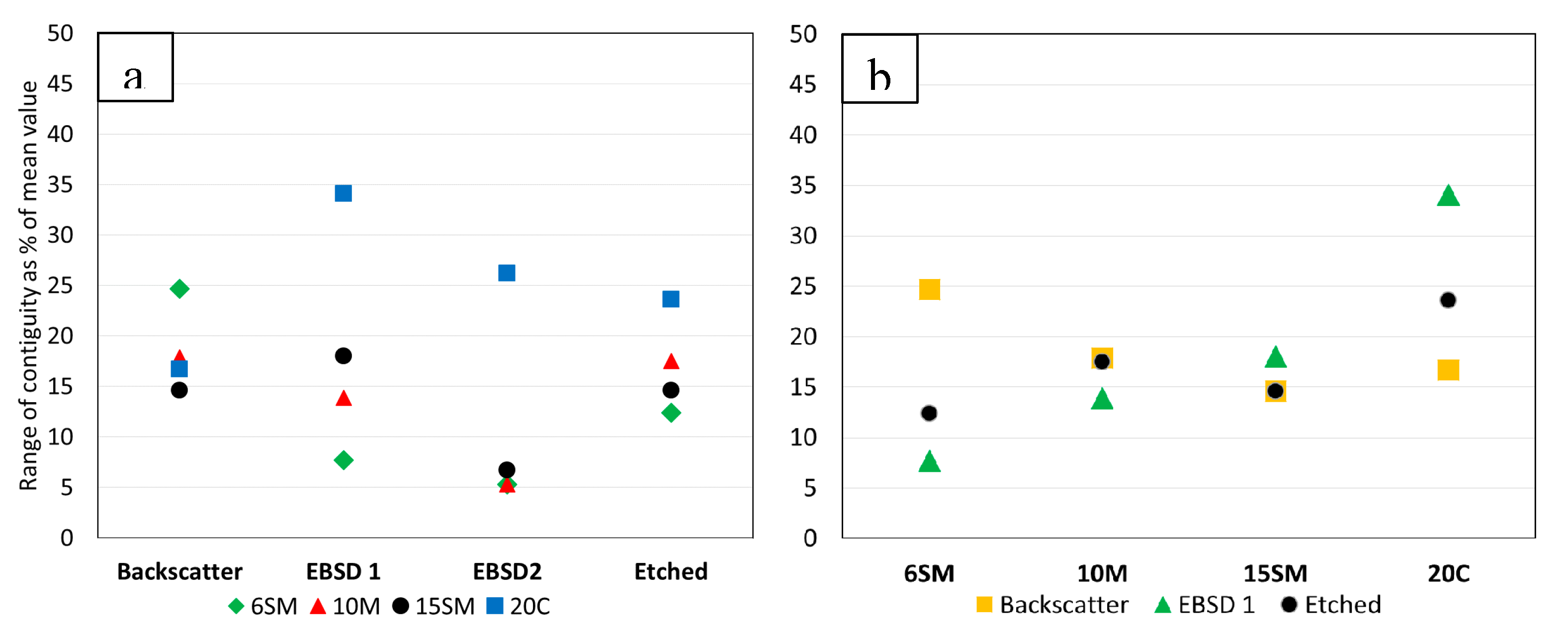
Figure 8 shows the scatter in results for all the results after removing outliers. As plotted, the scatter from the black background EBSD2 maps is noticeably lower than the other methods, but as noted previously, only 3 sets of measurements are included in determining the scatter so it is difficult to draw a definite conclusion. The other three methods are very similar in the variability of results with the exception, surprisingly, of the coarsest grade (20C), for which the EBSD greyscale map gives nearly 10% more variation.

Also surprising on initial examination is that the finest grade 6SM shows the reverse trend in variability for 20C, with EBSD greyscale having the lowest variation (8% of the mean value) and backscatter three times this level (25%). The requirement for a much higher resolution to measure the contiguity in the fine scale 6SM sample would be expected to cause more problems for identifying boundaries, while 20C would be expected to cause the least difficulty. It has to be presumed that the much greater number of WC-WC rather than WC-Co grain boundaries in 6SM means a) it is less sensitive to missed Co boundaries in EBSD maps and b) is more likely to have wrongly identified WC-WC boundaries in the backscatter image. Conversely, the 20C EBSD map is likely to have more WC-Co boundaries which are missed because of low resolution.

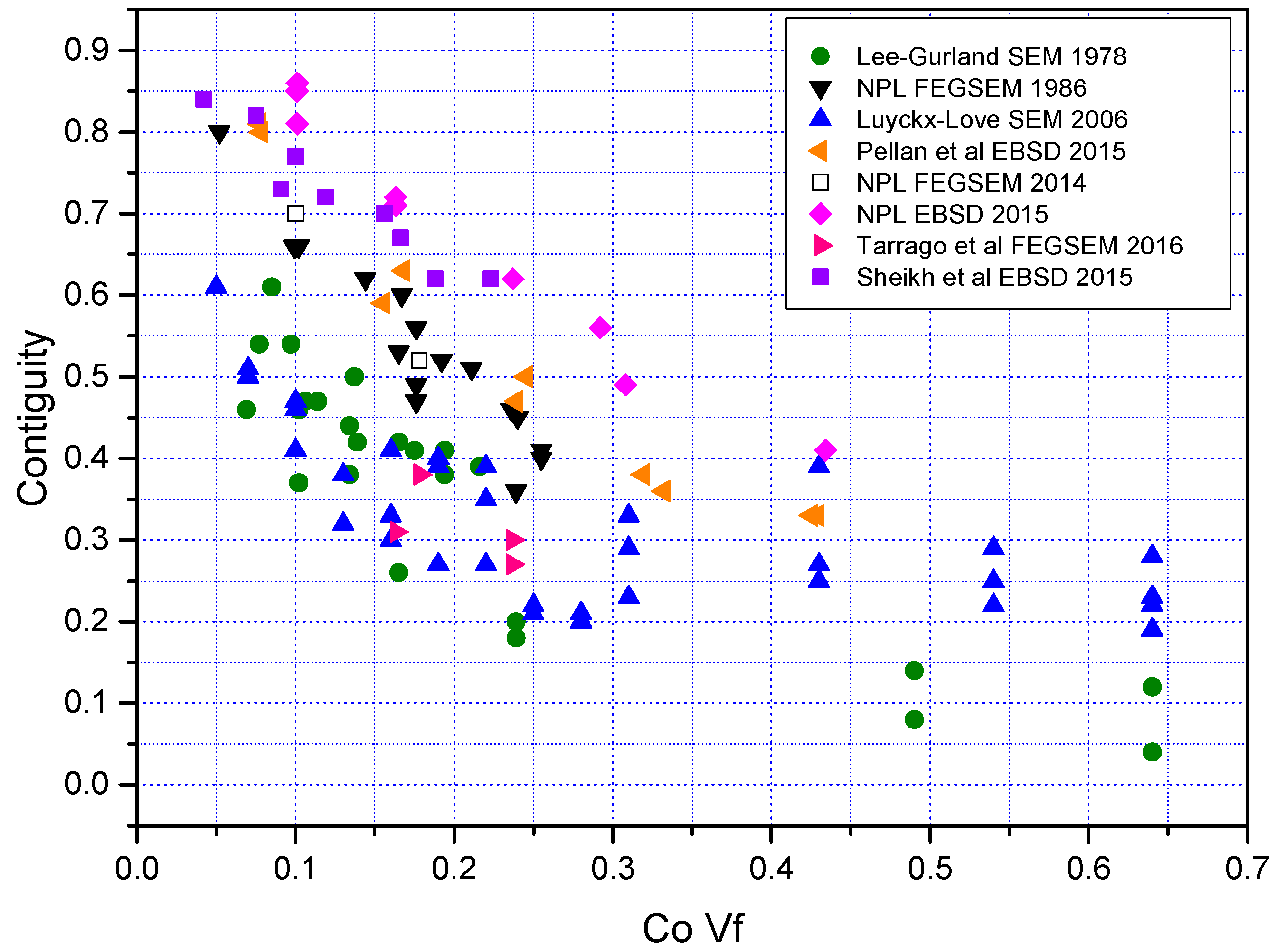
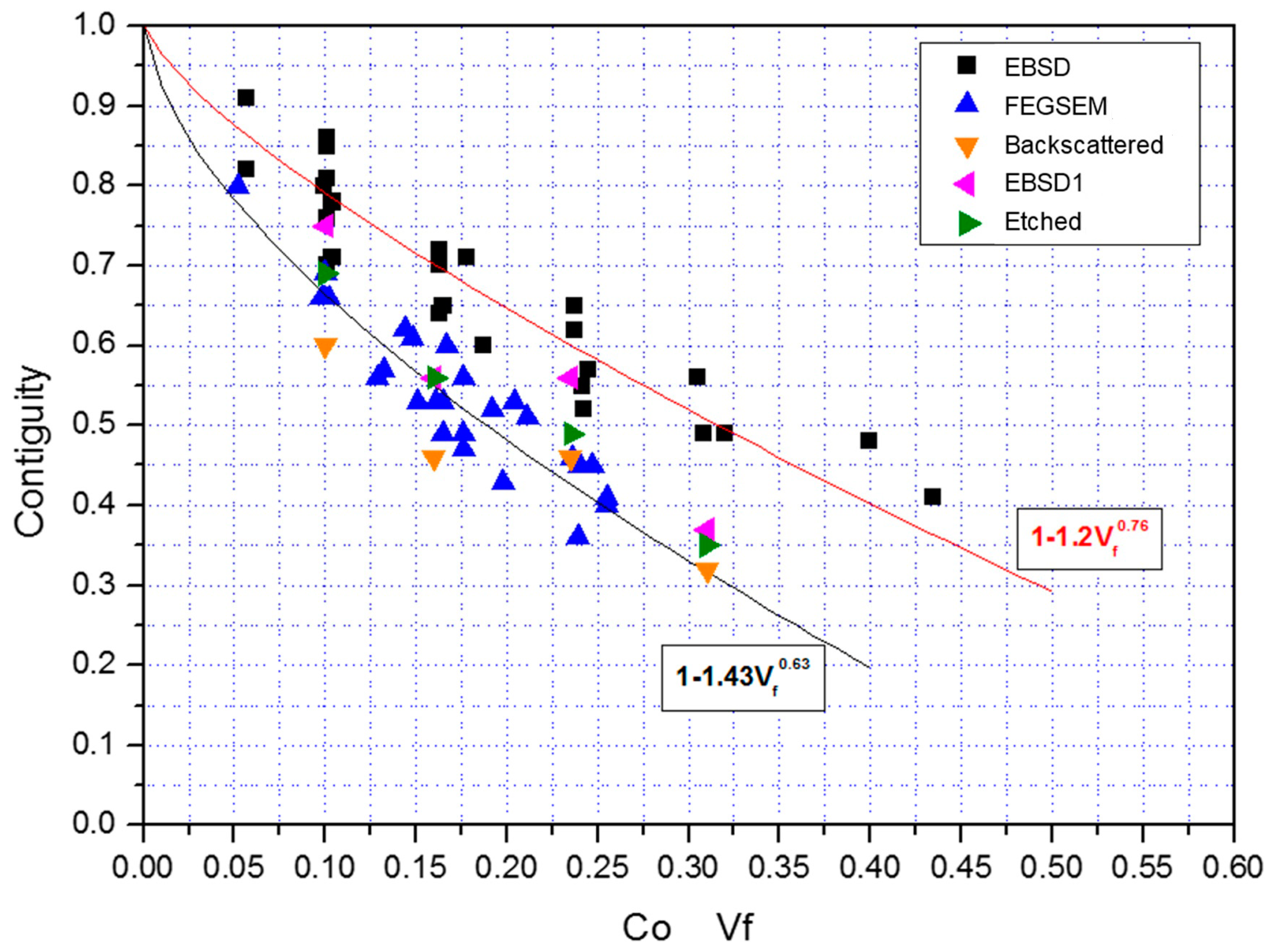
With the detailed information available from these interlaboratory tests, it is useful to compare the current results with earlier data from the literature. Figure 9 re-plots some of the data from Figure 1, showing the earlier high-resolution SEM image data and the EBSD data as two data sets. The interlab measurements from the backscattered and etched images and the first EBSD map set are plotted on top of the earlier data.

The data from the two interlab SEM image types, backscattered and etched, fall just about within the scatter of the earlier SEM image data. The backscattered images were generally on the low end and the etched images at the high end of the earlier data spread.

The interlab EBSD data were toward the lower end of the earlier EBSD data spread, particularly for the two coarser grades (10 wt.% and 20 wt.% equivalent to 16 vol.% and 31 vol.%). For these two coarser grades, these EBSD contiguity measurements were closer to the range of the earlier SEM data.

The data from the interlab and the images in Figure 5 show that EBSD is clearly limited by the resolution possible with this technique which results in the smallest features being missed. As these smallest features affect more Co-WC than WC-WC boundaries, contiguity is overestimated. Resolution limits will obviously affect the finer grain size materials but coarser grades are also affected by the pixel/step size chosen to map an area within a practical time. All grades are also strongly influenced by the map quality and subsequent “clean up” methods used on poorly indexed pixels.

The interlaboratory EBSD contiguity values were all on or significantly below the lower bound of earlier published EBSD results which suggests the quality and clean up factors were probably the greatest reason for the much higher EBSD contiguity in earlier published results. The reduction in the over-estimation achieved with the interlab EBSD resulted from the high-quality ion beam polished surfaces used which allow good indexing of both Co and WC. Earlier EBSD mapping has generally been on mechanically polished samples in which differential polishing led to recessing and shadowing of the Co and often much poorer indexing of the Co as well, resulting in poorer identification of the WC-Co boundaries.

In the results, the ion beam polished backscattered images were used as a baseline because they were felt to give the most accurate representation of the true structure. However, further work is needed to verify if some WC-WC boundaries are still missed in backscattered images. If they are being missed then it would account for the lower contiguity measured. EBSD mapping of a backscattered image area could produce this verification.

Even if the above verification is carried out, it also remains the case that etching is a simpler and more widely used method than ion beam polishing, and the scatter in results was similar for both techniques. Therefore, for the immediate future, etching combined with high-resolution SEM imaging should remain the chosen method of identifying grain boundaries and hence for contiguity measurement. Secondary electron imaging is normally used for etched samples, but if backscattered images can be obtained of the etched samples without excessive topographic contrast, then this imaging technique should be used. EBSD will only give comparable results on coarse grained (i.e., >1.5 µm mean size) if samples have been ion beam polished.

Whichever method is used, the interlaboratory data shows that any contiguity value reported has an uncertainty of about ±10% just to allow for variability between different people making a measurement. Improvements on this uncertainty might be achieved with agreed examples of how to interpret linear intercepts that are close to or touching triple points or ambiguous features. Ultimately an automated image analysis technique is desirable, but this probably requires the ability to combine very high quality backscattered images with EBSD data.

Figure 9 showed that a reasonable curve fit can be obtained for the FEGSEM data which links contiguity to Co volume fraction, V_f.

$$C=1-1.43 V_f^{0.63}$$

(2)

Although the curve gives correctly a contiguity of 1 for no binder phase, care should be taken in extrapolating outside the range shown in Figure 9, i.e., for 0.05 < V_f < 0.35. The upper curve and equation in Figure 9 is a fit to the EBSD data only. At low volume fractions resolution becomes even more important for detecting small regions of Co, and at high volume fractions clustering of WC, grains can occur which would make a single value of C meaningless. Nevertheless, the model can be useful for the provision of guideline values for studies of both mechanical properties as well as thermal and electrical conduction.

4. Conclusions

Ion beam polishing of hardmetals combined with backscattered electron imaging provides the most reliable images of the microstructure suitable for measurement of the microstructural contiguity.

Measurement of structure from EBSD maps is highly likely to lead to an overestimation of contiguity, largely because EBSD maps do not have the resolution of SEM images to identify small binder phase regions between WC grains. Only if a particularly long EBSD mapping run with a very fine step size is used will a contiguity value be obtained which is close to an SEM image measurement. For fine grained materials (0.5 µm and below) it will be almost impossible for EBSD to have sufficient resolution to identify all the binder phase regions needed for an accurate measurement. This problem is increased when the hardmetal has not been polished with an ion beam to minimise differential removal of the binder phase. In the longer term, combining reasonably high-resolution EBSD maps with backscattered images from ion beam polished samples may prove to provide a successful image from which to obtain a useful measurement of contiguity.

Although ion beam polishing provides the best images, it is recommended that, as etching is much more widely available and it gives results close to ion beam polishing, high-resolution imaging of a lightly etched WC surface could be an approved method for measurement of contiguity. An even better approach is to combine this latter process with a backscattered image where possible. However, even with good images, variation between operators is likely to lead to an uncertainty of approximately ±10%.