Article

Modeling of Ti6Al4V Alloy Orthogonal Cutting with Smooth Particle Hydrodynamics: A Parametric Analysis on Formulation and Particle Density

by
Adam D. Lampropoulos
*,
Angelos P. Markopoulos
and
Dimitrios E. Manolakos
Laboratory of Manufacturing Technology, School of Mechanical Engineering, National Technical University of Athens, Heroon Polytechniou 9, 15780 Athens, Greece
*
Author to whom correspondence should be addressed.
Metals 2019, 9(4), 388; https://doi.org/10.3390/met9040388
Submission received: 27 February 2019 / Revised: 15 March 2019 / Accepted: 22 March 2019 / Published: 28 March 2019
(This article belongs to the Special Issue Failure Mechanisms in Alloys)

Abstract

:
Computational modeling is a widely used method for simulation and analysis of machining processes. Smooth particle hydrodynamics (SPH) is a comparatively recently developed method that is used for the simulation of processes where high strains and fragmentation occur. The purpose of this work is the application of the SPH method for the prediction of cutting forces and chip formation mechanism in orthogonal cutting of Ti6Al4V alloy. In addition, it is examined how the final results of the simulation are influenced by the choice of the particular formulation of the SPH method, as well as by the density of the particles.

1. Introduction

Titanium alloys due to their unique mechanical properties are widely used in industrial applications. Especially, the Ti6Al4V alloy is one of the most widely used alloys and constitutes more than 50% of titanium products globally [1]. Most applications of this alloy are found in the aerospace industry, but it is also used for the production of medical devices due to its biocompatibility. However, it exhibits particular attributes as a material, such as low thermal conductivity, high strength at elevated temperatures, and low modulus of elasticity which lead to low machinability ratings [2,3]. Machining is one of the most prevalent processes for the production of industrial components and, due to the reasons mentioned above, cutting of titanium is usually accompanied by high cutting forces and high cutting temperatures. These major factors lead to excessive tool wear, shortened tool life, and poor surface quality of the final workpiece.
In practice, to increase productivity and at the same time keep quality at a high level, it is always necessary for the proper machining parameters to be chosen. There are mainly two ways that this goal can be attained. The first one involves conducting experiments to accumulate knowledge on the dependence of machining conditions upon important physical quantities (cutting forces, temperature etc.) during cutting. The second way involves the simulation of the machining process through the development of computational models. During the last decades, simulations have become increasingly popular and allow researchers to analyze, study, and understand in depth the physics of machining.
The finite element method (FEM) is one of the most frequently used numerical techniques for engineering simulations. However, there are a number of difficulties that arise when it is used for cutting simulations. Firstly, large strains lead to severe element distortions and consequently to the termination of the simulation, due to negative volume elements. Secondly, in order to model the fracture of the workpiece, a failure criterion has to be implemented into the code, so that certain elements are deleted from the grid when certain criteria are satisfied. The problem of distorted elements is usually solved with remeshing algorithms, which recreate the mesh after a user-defined number of time steps, resulting in increased computational cost. An alternative solution to this problem is based on element erosion/deletion when the stresses or strains inside an element surpass a certain threshold. The disadvantage of this approach is the fact that many elements can be artificially deleted from the grid, leading to non-physical simulations.
In [4], the orthogonal cutting is simulated by the FEM where a simple geometric criterion, combined with a mesh rezoning algorithm is used for the modeling of material separation. In [5,6,7], fracture is simulated by an element deletion algorithm which is based on a fracture criterion. Also, avoidance of severe element distortion is overcome by the usage of remeshing algorithms. In [8,9,10], material separation in the simulations is modeled by the formation of adiabatic shear bands and the usage of fracture criterions is avoided. However, the usage of remeshing algorithms still remains a necessity for the same reasons. In [11], the influence of cutting conditions on the stress at the rear surface of the tool is investigated. In [12], a mathematical model for the calculation of cutting forces is developed, based on the results of a FEM model. In [13,14], the influence of the constitutive model and the damage criteria on the prediction of cutting forces is studied. An alternative to classical FEM techniques is the use of combined Lagrangian–Eulerian formulations, where the grid is not tied on the workpiece but it is fixed in space [15,16,17].
During recent years, meshless numerical methods are gaining increased popularity because the particles/nodes are not strictly connected with their neighbor particles, but are relatively free to move in space, unlike the nodes of a finite element grid. In this study, the focus is on the smooth particle hydrodynamics meshless method. The SPH method was developed in the 1980s and was used for the numerical simulation of physical problems that belong to the field of astrophysics [18] and a decade later was modulated for solid mechanics problems [19]. A comprehensive analysis of the SPH method and examples regarding its applications in solid and fluid mechanics can be found in [20,21].
One of the earliest implementations of the SPH method to orthogonal cutting simulations can be found in [22], where the benefits of the method are presented in comparison to the traditional FEM approach. In [23], a 2D model is presented where friction is predicted in workpiece/cutting tool interface without the usage of a friction model, since both bodies are modeled with SPH particles. In [24], a model of the same type is used for the prediction of the variation of cutting forces caused by a worn cutting tool. In [25,26,27,28,29,30], SPH models of orthogonal, or oblique, cutting are created where the cutting tool is modeled with finite elements and the workpiece with SPH particles, which means that a friction model had to be used. In [30], the effect of subsequent cuts on the evolution of residual stresses in the workpiece is presented. Studies of SPH simulations regarding the influence of factors describing the material behavior such as the friction coefficient, the equation of state, or the usage of a damage-evolution criterion can be found in [31,32,33]. The influence of more intrinsic parameters to the SPH method, such as timestep and particle density, can be found in [34]. Similarly, in [35] the effect of important SPH control parameters is examined.
One of the deficiencies of the SPH method in metal cutting simulations is the inability of prediction of a realistic chip curvature, as it is mentioned in [36]. For this reason, alternative formulations are proposed to the standard SPH scheme, where this issue is resolved. One of these formulations is called renormalization and more details about its foundations and development can be found in [37,38]. Orthogonal cutting simulations with SPH can be found in the literature [23,24,25,26,27,28,29,30,31,32,33,34,35] for different formulations. However, there are no studies that examine the influence of the chosen formulation, on the prediction of the cutting forces. The aim of this study is the investigation of the differences in the prediction of cutting forces between two different formulations. For this purpose, numerical simulations of orthogonal cutting of Ti6Al4V titanium alloy are presented, where both formulations are used, namely the standard and the renormalized. This parametric analysis is complemented by conducting numerical simulations with different particle densities.
In Section 2, the mathematical foundations of SPH are summarized. The presentation of the theory in this section is based on [21]. In Section 3, the main formulas describing the material behavior are also provided, while in Section 4, the configuration of the numerical simulation is described. Furthermore, the way the parametric analysis was conducted, is described in detail. In Section 5, the main results of the parametric analysis are presented. For all the simulations, the commercial solver LSDYNA [39] was used.

2. SPH Foundations

In the SPH method, a function is represented by the following integral
f ( x ) = Ω f ( x ) δ ( x x ) dx
where δ ( x x ) is the Dirac delta function, which can be approximated by a smoothing function W(x − x′, h) that is chosen to fulfill a number of properties.
(a) The first property is the compact condition
W(x − x′, h) = 0, if |x − x′|>κh
where h is the smoothing length and κ is a constant that affects the non zero area centered around point x .
(b) The second property that the smoothing function fulfills is the fact that it converges to the Dirac function
lim h 0 W ( x x , h ) = δ ( x x )
(c) The final property that usually is fulfilled is the normalization condition
Ω W ( x x , h ) d x = 1
The integral representation in Equation (1) is replaced by the equation
< f ( x ) > = Ω f ( x ) W ( x x , h ) d x
where <   > is called the kernel approximation operator. Since the function W is zero for points outside a sphere with center at x and radius κ h , it is possible to replace the problem domain Ω with the support domain R = { x R 3 : | x x | κ h } . For the evaluation of the function in Equation (2), a numerical integration is carried out over a finite number of points in the neighborhood of x . In SPH, these points are represented by particles; each of them is considered to occupy a distinct amount of space and have a distinct mass. As can be seen from Figure 1, the particle X i is positioned at the center of the support domain R of function W . For the numerical integration of Equation (2) the following sum has to be evaluated
< f ( X i ) > = j = 1 N f ( X j ) W ( X j X i , h ) V j .
where N is the number of neighbor particles j inside the support domain and V j is the volume of each particle. Since each particle has a separate mass, the volume is substituted by the relation
V j = m j / ρ j
So, Equation (3) can be rewritten as
< f ( X i ) > = j = 1 N f ( X j ) W ( X j X i , h ) m j ρ j
It is worth mentioning that the density at point X i is the weighted average of the masses of the neighbor particles, i.e.,
ρ ( X i ) = j = 1 N m j W ( X j X i , h )
Since many smoothing functions fulfill the aforementioned properties (a–c), there is a variety of different functions proposed over the years. A smoothing function, except properties a to c, is necessary to have a small support domain, which means that it converges to zero quickly and also it is important to have smooth derivatives. In this study, the commercial solver LS-DYNA Ver.R10.1.0.rev.123264 [39] is used for the numerical simulations, in which the cubic B-spline is chosen as a smoothing function. The B-spline was proposed in [40] and is one of the most widely used kernels, since it is numerically efficient due to its small support domain.
W ( x x , h ) = 1 π h 3 { 1 2 3 u 2 + 3 4 u 3 , 0 u 1 1 4 ( 2 u ) 3 1 u 2 0 u > 2
where u = | x x | / h .

3. Material Modeling

3.1. Constitutive Model

For the mathematical modeling of the mechanical behavior of the workpiece material, the Johnson–Cook (J–K) constitutive relation was chosen. The Johnson–Cook model can be found in MAT_015 card [39] of LS-DYNA
σ eq = ( A + B ε eq n ( 1 + cln ε ˙ eq * ) C ( 1 T * m )
where, σ eq is the Von Misses equivalent stress, ε eq the equivalent strain, ε ˙ eq * the equivalent strain rate divided by a reference strain rate ε ˙ eq * = ε ˙ eq / ε ˙ 0 and stands for the homologous temperature T * = ( T T r ) / ( T m T r ) , where T r is the room temperature and T m is the melting temperature. Also, A, is the initial yield stress of the material, B, is the hardening constant, n, is the hardening exponent, C, is the strain rate constant and, m, is the thermal softening exponent. The values chosen for the parameters of the J–K model greatly affect the results of cutting simulations and the values provided in the literature for the same material vary among different authors. The values chosen in this study are provided from [41] and can be seen in Table 1. This choice is reported in [42], where it is shown that this set of parameters for the material model, provides the most accurate results for the cutting force. Also, the J–K model is used only for the workpiece since the cutting tool, due to its relatively great stiffness, is modeled as a rigid body.

3.2. Equation of State

Apart from the constitutive model, it is necessary to define the material pressure by relation to the density of the material. In LS-DYNA the simplest equation of state is the linear polynomial equation [39], where the pressure is related to the density with the relation
P = C 0 + C 1 μ + C 2 μ 2 + C 3 μ 3 + ( C 4 + C 5 μ + C 6 μ 2 ) E
where μ = ( ρ ρ 0 ) / ρ 0 . If C 0 = C 2 = C 3 = C 4 = C 5 = C 6 = 0 , then C 1 is equal to the bulk modulus, since P = K μ . Although the linear polynomial is considered a simplified model, it has been shown that the final results do not vary considerably when more accurate state equations are used [32].

3.3. Material Separation Modelling

For the proper simulation of cutting processes, the implementation of material separation by fracture or adiabatic shear banding is necessary. In traditional finite element codes, a fracture criterion, combined with an element deletion algorithm, is frequently used for elements located inside the material separation zone to be deleted. In the SPH method, the simulation of processes, where severe strains occur, can be modeled without the usage of a fracture criterion, since the SPH particles are loosely connected. In other words, the nodes of a finite element are strictly connected, regardless of the distance between each other; the element has to be deleted if their disconnection is necessary. On the contrary, a particle in the SPH code is affected by the neighbor particles that lie inside the support domain and there is not a predetermined connection between certain particles.

3.4. Contact and Friction Modeling

In this study, the frictional forces are considered to follow the Coulomb law
τ = f σ n
where τ is the frictional stress and σ n is the normal stress. The friction coefficient f is constant over the entire contact area. In LS-Dyna, the friction coefficient can be defined in the AUTOMATIC-NODES-TO-SURFACE card. Also, on the same card, contact between the workpiece and the cutting tool is defined. A penalty type algorithm is used so that the particles of the workpiece remain in the exterior of the cutting tool’s boundaries.

4. Numerical Simulation Configuration

Due to its relative simplicity, most published research is concerned with the simulation of orthogonal cutting. However, the results of a simulation need to be validated by actual experimental data and orthogonal cutting is not a widely used process in practice. Therefore, in many studies experimental data is derived from actual machining operations. Machining processes are mainly 3-dimensional and can be approximated by a 2-dimensional process to a certain extent. In this study, experimental results from reference [43] are used, where actual orthogonal cutting is conducted.
In the experimental reference, the cutting tool is moving with constant speed V into a flat strip of width Wc = 1 mm, height H = 2 mm and a length L = 10 mm. The experiment is repeated for three depths of cut hc = 0.06, 0.04 and 0.1 mm. The material of the cutting tool is WC/Co tungsten carbide and of the workpiece Ti6Al4V titanium alloy (Table 2). The experimental conditions are summarized in Table 3.
The simulation set up can be seen in Figure 2. The height of the workpiece H is three times the depth of cut (H = 3 hc) and the width of the strip Wc is 0.01 mm. The length of the workpiece L is 1.5 mm, when the depth of cut is hc = 0.1 mm and is reduced to 1 mm for the remaining two values of hc. For the cutting tool and for the lower part of the workpiece up to one third its height, finite elements are used, and the rest of the workpiece is modeled with SPH particles. The nodes at the bottom and the edge of the strip are constrained in all directions.
The simulation of the experiment with the actual strip length is, from a computational standpoint, time-consuming and also unnecessary since the cutting process transitions to a steady state, where the cutting forces are stabilized long before the cutting tool reaches the end of the strip. The same applies for the width of the workpiece because all nodes are constrained to the z direction and are free to move in the x-y plane; it is redundant for the actual width of the workpiece to be modeled and scaling of the cutting forces to a factor of 100 is preferable. Finally, the SPH method is computationally more demanding than the standard FEM, and this is the reason why it is usually preferred for the area close to the path of the cutting tool to be modeled with particles. For the other parts, finite elements are considered more suitable and the mesh becomes gradually coarser at the bottom of the workpiece.
The parametric analysis is conducted based upon two parameters, the SPH formulation and the density of the particles. Initially, the distance d between the particles and the depth of cut hc are fixed to a certain value and the simulation is carried out twice. Initially, a standard SPH formulation is used, followed by a renormalized formulation.
Consequently, the simulation with the renormalized formulation is carried out once again and the particle distance d is reduced to half of the initial value. Afterward, a different value for the depth of cut hc is selected and the same procedure is repeated.

5. Results and Discussion

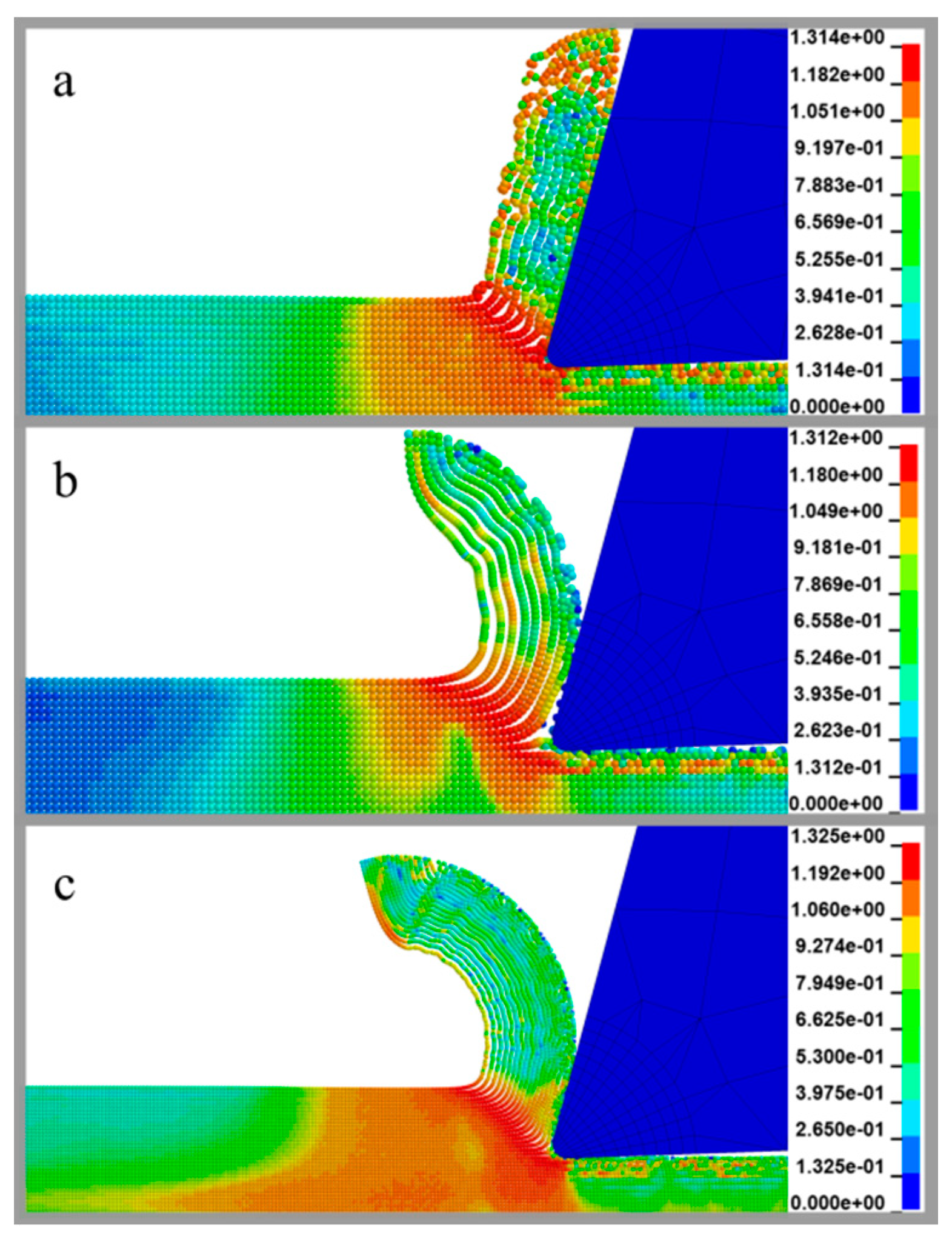
In Figure 3, the equivalent stress contours are depicted for a fixed depth of cut hc = 0.04 mm. In Figure 4 and Figure 5, the stress contours are shown for depths of cut of hc = 0.06 and 0.1 mm, respectively. By comparing the frames a and b for each depth of cut, an obvious observation is the chip curvature. By using the standard SPH formulation, a straight numerical chip is produced that follows the chip face of the cutting tool. The usage of the renormalized formulation leads to the production of a more realistic chip. The nonrealistic chip curvature of the standard formulation is attributed to the absence of particles in the exterior areas of the boundaries of the solution domain (workpiece) [36]. This absence leads to non-approximate calculations near the boundaries.
As can be seen in Figure 3b,c, the chip curvature is increased for a greater particle density and the same observation applies and for the other two values of the depth of cut. In contrast, the maximum stress is not affected considerably, regardless of the depth of cut, the formulation or the density of the particles. This can be explained by the fact that the maximum stress that is induced on the workpiece in the primary shear stress zone is dependent on the strength of the material.
In Figure 6, the plastic strain contours are depicted for each value of the depth of cut. In this figure, only the chips that are produced by the renormalized SPH are chosen, with the greater particle density. The areas with the larger values of strain can be seen at the secondary shear zone at the interface between the cutting tool and the chip, at the tertiary shear zone where the cutting tool rubs the surface of the workpiece, and also at the shear zones that are created at the primary shear zone.
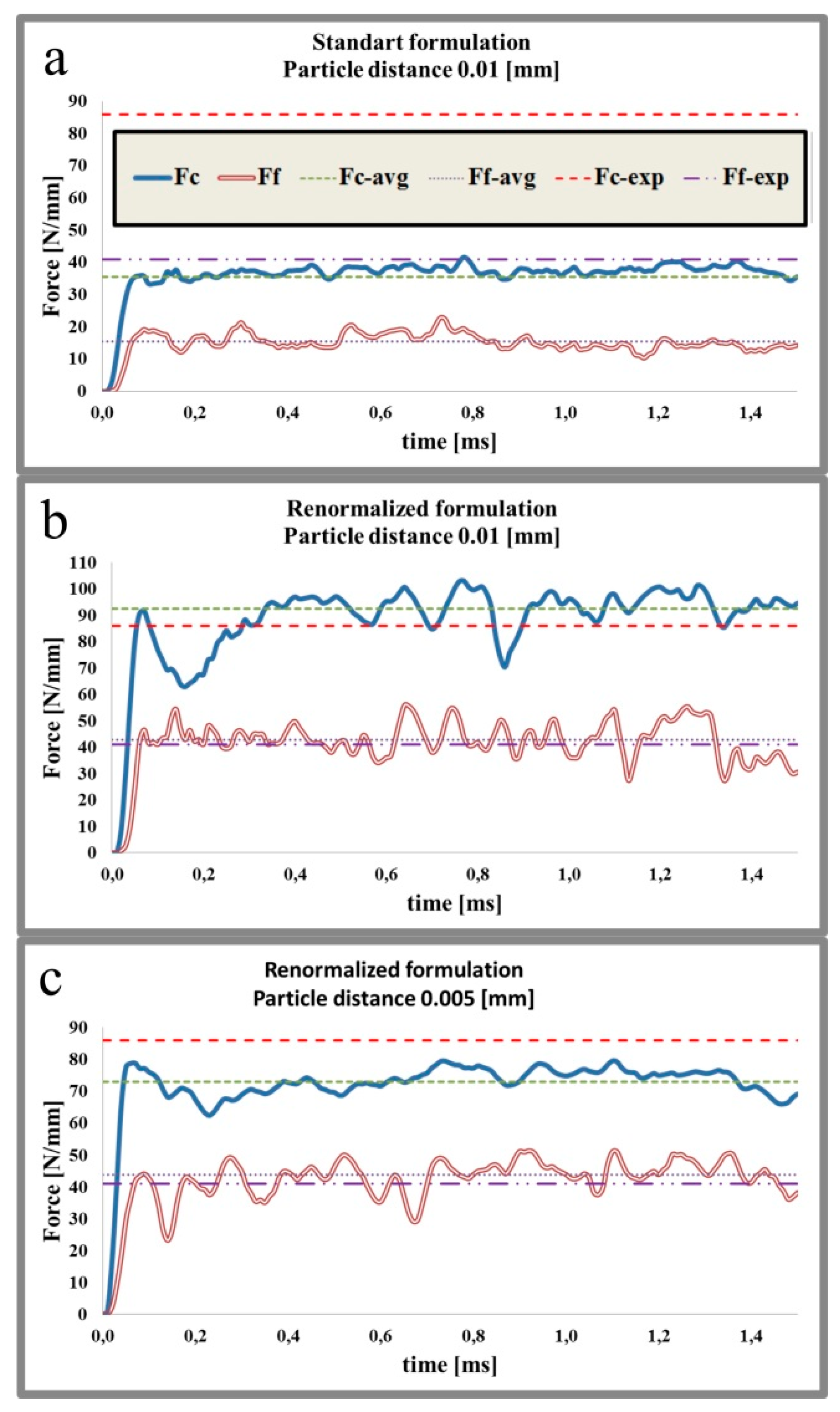
In Figure 7, Figure 8 and Figure 9, the cutting force Fc and the feed force Ff are depicted in relation to time. Each figure corresponds to one of the three values for the depth of cut. Also, as can be seen from these figures, the forces start to stabilize at the time of 0.1 to 0.3 ms. For the values depicted in each of these figures, an average value is computed from the time that the forces remain relatively stable until the end of the simulation. The average values are compared to the experimental ones.
As shown in Figure 7a, the results of the standard SPH scheme are not satisfactory since the predicted values are less than half the values of the experimental ones. In contrast, the values predicted by the renormalized formulation, which are depicted in Figure 7b, are very close to the experimental ones. The cutting force Fc and feed force Ff are overpredicted with an error of about 7.56% and 4.39%, respectively. By comparing Figure 7b with Figure 7c, it is obvious that the forces predicted by the model with greater particle density are more stable and oscillate less. In addition, lower values are predicted for the cutting force Fc and there is also a small increase in the feed force Ff. The cutting force Fc is underpredicted with an error of about 15% and the feed force Ff is overpredicted with an error of 6.8%.
As can be seen in Figure 8a and Figure 9a, the results produced from the standard SPH formulation remain far from the experimental values regardless of the depth of cut. By comparing Figure 8b to Figure 8c and Figure 9b to Figure 9c, the same pattern is observed. The models with greater particle density provide relatively decreased values for the cutting force Fc and increased values for the feed force Ff. Also, especially for the cutting forces, there is less variation between the maximum and minimum values. For a depth of cut of hc = 0.06 mm, the cutting force Fc is overpredicted with an error of 7.9%, the feed force Ff is underpredicted with a divergence of 20% from the experimental value. By increasing the number of particles, the predicted value of the cutting force Fc is lower than the experimental and the error is increased slightly to 9%. The predicted value for the feed force Ff is increased and almost coincides with the experimental value. For a depth of cut of hc = 0.01 mm, as can be seen in Figure 9, the averaged predicted cutting force Fc is very close to the experimental value and they differentiate by less than 1.2%. However, the model which is comprised of a greater number of particles underpredicts the cutting force Fc with an error of 10.4%. For both models, as can be seen from Figure 9b,c, the feed force Ff is underpredicted and the averaged values differ from the experimental with a percentage of 25%.
The numerically predicted cutting and feed forces are gathered in Table 4 and Table 5. At this point, it is obvious that only models where the renormalized formulation is used provide results close to the experimental values. Also, there is a negative correlation between cutting forces Fc and particle density. Models with smaller particle density estimate the cutting forces more accurately, which is an indication that the SPH models might converge to a value different from the experimental; still, the maximum deviation does not exceed 15%. For the feed forces Ff, a clear pattern is not visible. Although there is a positive correlation between feed force and particle density, the sensitivity is almost zero for hc = 0.1 mm and there is a slight change of the predicted values for hc = 0.04 mm, but for hc = 0.06 mm, the deviation between the feed forces estimated by the different particle density models approaches 26%. Generally, the cutting force Fc is estimated more accurately comparing to the feed force Ff and this can be attributed to the parameters chosen for the J–K model. As mentioned in reference [42], parameters provided in the literature for the J–K model usually do not lead to accurate estimations of both cutting and feed forces as well.

6. Conclusions

The orthogonal cutting of Ti6Al4V alloy was modeled by using the smooth particle hydrodynamics method. The main focus of this study was the influence of the choice between two different SPH formulations (standard and renormalized) on the prediction of cutting and feed forces. It was found that the implementation of the renormalized formulation leads to a satisfactory prediction of cutting forces. In contrast, the predictions of the standard formulations deviate from the experimental values of more than 50%. In addition, the usage of the renormalized formulation leads to a more realistic estimation of the chip geometry and this may be the main reason for the large difference in the estimation of the cutting forces between the two formulations.
This study was also complimented by the investigation of the influence of particle density in the estimation of chip geometry and cutting forces. From the results, it is evident that the curvature of the numerical chip increases when a greater number of particles is used. Also, models with more particles predict lower values of cutting forces and larger values for the feed forces.
Due to the meshless nature of this method, modeling of material separation was possible without the implementation of a fracture criterion or a remeshing algorithm. Because of these advantages, programming of the SPH method for cutting simulations is easier. Fracture criterions require calibration from experiments and element deletion algorithms may lead to an unrealistic mass loss in the simulation. Furthermore, remeshing algorithms are computationally demanding. Thus, SPH is a promising alternative to a classical FEM.

Author Contributions

Conceptualization, A.D.L., A.P.M., and D.E.M.; Formal analysis, A.D.L. and D.E.M.; Investigation, A.D.L.; Methodology, A.D.L. and A.P.M.; Resources, D.E.M.; Software, A.D.L. and A.P.M.; Supervision, D.E.M.; Validation, A.D.L.; Writing—original draft, A.D.L.; Writing—review and editing, A.P.M. and D.E.M.

Funding

This research received no external funding.

Conflicts of Interest

The authors declare no conflict of interest.

Nomenclature

AInitial yield stress [MPa]
B Hardening constant [MPa]
C Strain Rate Constant
dDistance between particles [mm]
E Young’s Modulus [GPa]
F c Cutting Force [N/mm]
F f Feed Force [N/mm]
fFriction coefficient
HHeight of the workpiece [mm]
hSmoothing length [mm]
hcDepth of cut [mm]
K Bulk modulus [GPa]
L Length of the workpiece [mm]
mThermal softening exponent
m j Mass of particle j
nHardening exponent
P Pressure [GPa]
r Cutting edge radius [μm]
T r Room temperature [K]
T m Melting temperature [K]
V Cutting speed [m/s]
WcWidth of the workpiece
W Kernel function
X i Position vector of particle i
x Position vector of a point in space
αClearance angle [deg]
γRake angle [deg]
δ Dirac function
V j Volume of particle j
ε eq Equivalent strain
ε ˙ eq Equivalent strain rate [1/s]
ε ˙ r e f Reference strain rate [1/s]
μ Relative change of density
ρDensity [ Kg / m 3 ]
ρ j Density of particle j
σ n Normal stress [GPa]
σ eq Equivalent stress [GPa]
τ Frictional stress [GPa]

References

  1. Welsch, G.; Boyer, R.; Collings, E.W. (Eds.) Materials Properties Handbook: Titanium Alloys; ASM International: Materials Park, OH, USA, 1994; ISBN 978-0-87170-481-8. [Google Scholar]
  2. Davim, J.P. (Ed.) Machining of Titanium Alloys; Springer: New York, NY, USA, 2014; ISBN 978-3-662-43901-2. [Google Scholar]
  3. Ezugwu, E.O.; Wang, Z.M. Titanium alloys and their machinability—A review. J. Mater. Process. Technol. 1997, 68, 262–274. [Google Scholar] [CrossRef]
  4. Mamalis, A.G.; Horváth, M.; Branis, A.S.; Manolakos, D.E. Finite element simulation of chip formation in orthogonal metal cutting. J. Mater. Process. Technol. 2001, 110, 19–27. [Google Scholar] [CrossRef]
  5. Ng, E.-G.; Aspinwall, D.K. Modelling of hard part machining. J. Mater. Process. Technol. 2002, 127, 222–229. [Google Scholar] [CrossRef]
  6. Guo, Y.B.; Yen, D.W. A FEM study on mechanisms of discontinuous chip formation in hard machining. J. Mater. Process. Technol. 2004, 155–156, 1350–1356. [Google Scholar] [CrossRef]
  7. Hua, J.; Shivpuri, R. Prediction of chip morphology and segmentation during the machining of titanium alloys. J. Mater. Process. Technol. 2004, 150, 124–133. [Google Scholar] [CrossRef] [Green Version]
  8. Rhim, S.-H.; Oh, S.-I. Prediction of serrated chip formation in metal cutting process with new flow stress model for AISI 1045 steel. J. Mater. Process. Technol. 2006, 171, 417–422. [Google Scholar] [CrossRef]
  9. Calamaz, M.; Coupard, D.; Girot, F. A new material model for 2D numerical simulation of serrated chip formation when machining titanium alloy Ti–6Al–4V. Int. J. Mach. Tools Manuf. 2008, 48, 275–288. [Google Scholar] [CrossRef] [Green Version]
  10. Sima, M.; Özel, T. Modified material constitutive models for serrated chip formation simulations and experimental validation in machining of titanium alloy Ti–6Al–4V. Int. J. Mach. Tools Manuf. 2010, 50, 943–960. [Google Scholar] [CrossRef]
  11. Pimenov, D.Y.; Guzeev, V.I.; Koshin, A.A. Influence of cutting conditions on the stress at tool’s rear surface. Russ. Eng. Res. 2011, 31, 1151–1155. [Google Scholar] [CrossRef]
  12. Pimenov, D.Y.; Guzeev, V.I. Mathematical model of plowing forces to account for flank wear using FME modeling for orthogonal cutting scheme. Int. J. Adv. Manuf. Technol. 2017, 89, 3149–3159. [Google Scholar] [CrossRef]
  13. Ducobu, F.; Rivière-Lorphèvre, E.; Filippi, E. Influence of the Material Behavior Law and Damage Value on the Results of an Orthogonal Cutting Finite Element Model of Ti6Al4V. In Proceedings of the 14th CIRP Conference on Modeling of Machining Operations (CIRP CMMO), Turin, Italy, 13–14 June 2013; Settineri, L., Ed.; Elsevier: Amsterdam, The Netherlands, 2013; pp. 379–384. [Google Scholar]
  14. Boldyrev, I.S.; Shchurov, I.A.; Nikonov, A.V. Numerical Simulation of the Aluminum 6061-T6 Cutting and the Effect of the Constitutive Material Model and Failure Criteria on Cutting Forces’ Prediction. In Proceedings of the 2nd International Conference on Industrial Engineering (ICIE-2016), Chelyabinsk, Russia, 19–20 May 2016; Radionov, A.A., Ed.; Elsevier: Amsterdam, The Netherlands, 2016; pp. 866–870. [Google Scholar]
  15. Ducobu, F.; Arrazola, P.-J.; Rivière-Lorphèvre, E.; de Zarate, G.O.; Madariaga, A.; Filippi, E. The CEL Method as an Alternative to the Current Modelling Approaches for Ti6Al4V Orthogonal Cutting Simulation. In Proceedings of the 16th CIRP Conference on Modelling of Machining Operations (16th CIRP CMMO), Cluny, France, 15–16 June 2017; Outeiro, J., Poulachon, G., Eds.; Elsevier: Amsterdam, The Netherlands, 2017; pp. 245–250. [Google Scholar]
  16. Ducobu, F.; Rivière-Lorphèvre, E.; Filippi, E. Finite element modelling of 3D orthogonal cutting experimental tests with the Coupled Eulerian-Lagrangian (CEL) formulation. Finite Elem. Anal. Des. 2017, 134, 27–40. [Google Scholar] [CrossRef]
  17. Grissa, R.; Zemzemi, F.; Fathallah, R. Three approaches for modeling residual stresses induced by orthogonal cutting of AISI316L. Int. J. Mech. Sci. 2018, 135, 253–260. [Google Scholar] [CrossRef]
  18. Gingold, R.A.; Monaghan, J.J. Smoothed particle hydrodynamics: theory and application to non-spherical stars. Mon. Not. R. Astron. Soc. 1977, 181, 375–389. [Google Scholar] [CrossRef] [Green Version]
  19. Libersky, L.D.; Petschek, A.G. Smooth particle hydrodynamics with strength of materials. In Advances in the Free-Lagrange Method Including Contributions on Adaptive Gridding and the Smooth Particle Hydrodynamics Method; Trease, H.E., Fritts, M.F., Crowley, W.P., Eds.; Springer: Berlin, Germany, 1991; Volume 395, pp. 248–257. ISBN 978-3-540-54960-4. [Google Scholar]
  20. Liu, G.R. Meshfree Methods: Moving Beyond the Finite Element Method, 2nd ed.; CRC Press: Boca Raton, FL, USA, 2009; ISBN 978-1-4200-8210-4. [Google Scholar]
  21. Liu, G.R.; Liu, M.B. Smoothed Particle Hydrodynamics: A Meshfree Particle Method; World Scientific: Hackensack, NJ, USA, 2003; ISBN 978-981-238-456-0. [Google Scholar]
  22. Heinstein, M.; Segalman, D. Simulation of Orthogonal Cutting with Smooth Particle Hydrodynamics; SAND-97-1961; Sandia National Labs.: Albuquerque, NM, USA, 1 September 1997.
  23. Limido, J.; Espinosa, C.; Salaün, M.; Lacome, J.L. SPH method applied to high speed cutting modelling. Int. J. Mech. Sci. 2007, 49, 898–908. [Google Scholar] [CrossRef] [Green Version]
  24. Calamaz, M.; Limido, J.; Nouari, M.; Espinosa, C.; Coupard, D.; Salaün, M.; Girot, F.; Chieragatti, R. Toward a better understanding of tool wear effect through a comparison between experiments and SPH numerical modelling of machining hard materials. Int. J. Refract. Met. Hard Mater. 2009, 27, 595–604. [Google Scholar] [CrossRef] [Green Version]
  25. Villumsen, M.F.; Fauerholdt, T.G. Simulation of Metal Cutting using Smooth Particle Hydrodynamics. In Proceedings of the 7th LS-DYNA Anwenderforum, Bamberg, Germany, 30 September–1 October 2008; pp. 17–36. [Google Scholar]
  26. Bagci, E. 3-D numerical analysis of orthogonal cutting process via mesh-free method. Int. J. Phys. Sci. 2011, 6, 1267–1282. [Google Scholar]
  27. Dănuț, J. SPH Meshless Simulation of Orthogonal Cutting of AA6060-T6. Appl. Mech. Mater. 2015, 808, 258–263. [Google Scholar] [CrossRef]
  28. Spreng, F.; Eberhard, P. Machining Process Simulations with Smoothed Particle Hydrodynamics. In Proceedings of the 15th CIRP Conference on Modelling of Machining Operations, Karlsruhe, Germany, 11–12 June 2015; pp. 94–99. [Google Scholar]
  29. Umer, U.; Mohammed, M.K.; Qudeiri, J.A.; Al-Ahmari, A. Assessment of finite element and smoothed particles hydrodynamics methods for modeling serrated chip formation in hardened steel. Adv. Mech. Eng. 2016, 8, 1–11. [Google Scholar] [CrossRef]
  30. Geng, X.; Dou, W.; Deng, J.; Yue, Z. Simulation of the cutting sequence of AISI 316L steel based on the smoothed particle hydrodynamics method. Int. J. Adv. Manuf. Technol. 2017, 89, 643–650. [Google Scholar] [CrossRef]
  31. Madaj, M.; Píška, M. On the SPH Orthogonal Cutting Simulation of A2024-T351 Alloy. In Proceedings of the 14th CIRP Conference on Modeling of Machining Operations, Turin, Italy, 13–14 June 2013; Settineri, L., Ed.; Elsevier: Amsterdam, The Netherlands, 2013; pp. 152–157. [Google Scholar]
  32. Olleak, A.A.; El-Hofy, H.A. SPH Modelling of Cutting Forces while Turning of Ti6Al4V Alloy. In Proceedings of the 10th European LS-DYNA Conference, Würzburg, Germany, 15–17 June 2015. [Google Scholar]
  33. Takabi, B.; Tajdari, M.; Tai, B.L. Numerical study of smoothed particle hydrodynamics method in orthogonal cutting simulations – effects of damage criteria and particle density. J. Manuf. Process. 2017, 30, 523–531. [Google Scholar] [CrossRef]
  34. Heisel, U.; Zaloga, W.; Krivoruchko, D.; Storchak, M.; Goloborodko, L. Modelling of orthogonal cutting processes with the method of smoothed particle hydrodynamics. Prod. Eng. 2013, 7, 639–645. [Google Scholar] [CrossRef]
  35. Avachat, C.S.; Cherukuri, H.P. A Parametric Study of the Modeling of Orthogonal Machining Using the Smoothed Particle Hydrodynamics Method. In Proceedings of the ASME 2015 International Mechanical Engineering Congress and Exposition, Houston, TX, USA, 13–19 November 2015; ASME: Houston, TX, USA, 2015; p. V014T06A005. [Google Scholar]
  36. Limido, J.; Espinosa, C.; Salaun, M.; Mabru, C.; Chieragatti, R.; Lacome, J.L. Metal cutting modelling SPH approach. Int. J. Mach. Mach. Mater. 2011, 9, 177–196. [Google Scholar] [CrossRef]
  37. Randles, P.W.; Libersky, L.D. Smoothed Particle Hydrodynamics: Some recent improvements and applications. Comput. Methods Appl. Mech. Eng. 1996, 139, 375–408. [Google Scholar] [CrossRef]
  38. Vila, J.P. SPH Renormalized Hybrid Methods for Conservation Laws: Applications to Free Surface Flows. In Meshfree Methods for Partial Differential Equations II; Griebel, M., Schweitzer, M.A., Eds.; Springer: Berlin, Germany, 2005; Volume 43, pp. 207–229. ISBN 978-3-540-23026-7. [Google Scholar]
  39. Livermore Software Technology Corporation. LS-DYNA KEYWORD USER’S MANUAL; Livermore Software Technology Corporation: Livermore, CA, USA, 2017. [Google Scholar]
  40. Monaghan, J.J.; Lattanzio, J.C. A refined particle method for astrophysical problems. Astron. Astrophys. 1985, 149, 135–143. [Google Scholar]
  41. Seo, S.; Min, O.; Yang, H. Constitutive equation for Ti–6Al–4V at high temperatures measured using the SHPB technique. Int. J. Impact Eng. 2005, 31, 735–754. [Google Scholar] [CrossRef]
  42. Ducobu, F.; Rivière-Lorphèvre, E.; Filippi, E. On the importance of the choice of the parameters of the Johnson-Cook constitutive model and their influence on the results of a Ti6Al4V orthogonal cutting model. Int. J. Mech. Sci. 2017, 122, 143–155. [Google Scholar] [CrossRef]
  43. Ducobu, F.; Rivière-Lorphèvre, E.; Filippi, E. Experimental contribution to the study of the Ti6Al4V chip formation in orthogonal cutting on a milling machine. Int. J. Mater. Form. 2015, 8, 455–468. [Google Scholar] [CrossRef]
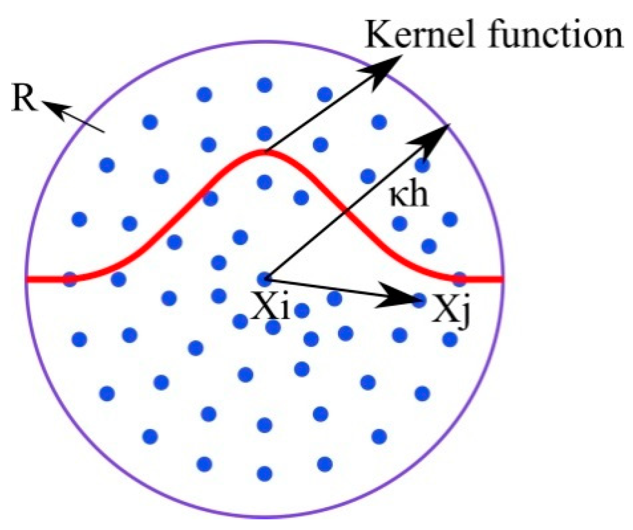
Figure 1. Support domain of kernel function centered at particle X i .
Metals 09 00388 g001
Figure 2. SPH model initial configuration.
Metals 09 00388 g002
Figure 3. Equivalent stress σeq contours in GPa for 0.04 mm depth of cut: (a) standard formulation and d = 0.01 mm; (b) renormalized formulation and d = 0.01 mm; (c) renormalized formulation and d = 0.005 mm.
Metals 09 00388 g003
Figure 4. Equivalent stress σeq contours in GPa for 0.06 mm depth of cut: (a) standard formulation and d = 0.01 mm; (b) renormalized formulation and d = 0.01 mm; (c) renormalized formulation and d = 0.005 mm.
Metals 09 00388 g004
Figure 5. Equivalent stress σeq contours in GPa for 0.1 mm depth of cut: (a) standard formulation and d = 0.01 mm; (b) renormalized formulation and d = 0.01 mm; (c) renormalized formulation and d = 0.005 mm.
Metals 09 00388 g005
Figure 6. Equivalent plastic strain εeq contours for a depth of cut hc: (a) 0.04 mm; (b) 0.06 mm; (c) 0.1 mm.
Metals 09 00388 g006
Figure 7. Cutting force Fc and feed force Ff versus time for hc = 0.04 mm.
Metals 09 00388 g007
Figure 8. Cutting force Fc and feed force Ff versus time for hc = 0.06 mm.
Metals 09 00388 g008
Figure 9. Cutting force Fc and feed force Ff versus time for hc = 0.1 mm.
Metals 09 00388 g009
Table 1. Material properties of the workpiece.
Material ParametersValues
A (MPa)997.9
B (MPa)653.1
C0.0198
m0.7
n0.45
ε ˙ r e f (s−1)1
T r   (K)298
T m   (K)1878
Young’s Modulus (E, GPa) 113.8
Density ρ ( kg / m 3 ) 4430
Friction coefficient (f)0.2
Table 2. The chemical composition of T1-6Al-4V titanium alloy according to AMS 4928 standard [1].
AlCFeHNOVOT
5.5–6.750.10.30.01250.050.23.5–4.50.4
Table 3. Experimental conditions described in (data from [43]).
Machining ParametersValues
Cutting speed V [m/s]0.5
Rake angle, γ [deg]15
Clearance angle, α [deg]2
Cutting edge radius r [μm]20
Depth of cut, hc [mm]0.040.060.1
Table 4. Comparison between predicted and experimental cutting forces Fc for all models.
Depth of Cut hc [mm]Experimental Cutting Force [N/mm]Standard Formulation (d = 0.01 [mm])
[N/mm]
Renormalized Formulation
(d = 0.01 [mm])
[N/mm]
Renormalized Formulation
(d = 0.005 [mm]) [N/mm]
0.048635.692.573
−58.6%+7.6%−15.1%
0.0611253,76120.9101.9
−52%+7.94%−9.02%
0.117386175155
−50.3%+1.2%−10.4%
Table 5. Comparison between predicted and experimental feed forces Ff for all models.
Depth of Cut hc [mm]Experimental Feed Force [N/mm]Standard Formulation (d = 0.01 [mm])
[N/mm]
Renormalized Formulation
(d = 0.01 [mm])
[N/mm]
Renormalized Formulation
(d = 0.005 [mm]) [N/mm]
0.044115.542.843.8
−62,2%+4.39%+6.8%
0.064514.935.9545.1
−66,9%−20.1%0.2%
0.15118.1538.3938.6
−64.4%−24.7%−24.3%