Microstructure, Mechanical Properties, and Constitutive Models for Ti–6Al–4V Alloy Fabricated by Selective Laser Melting (SLM)


Abstract
1. Introduction
2. Materials and Methods
3. Results and Discussion
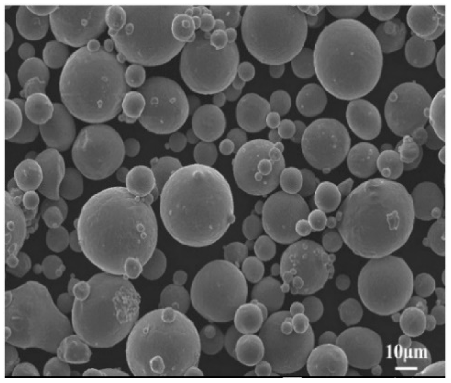
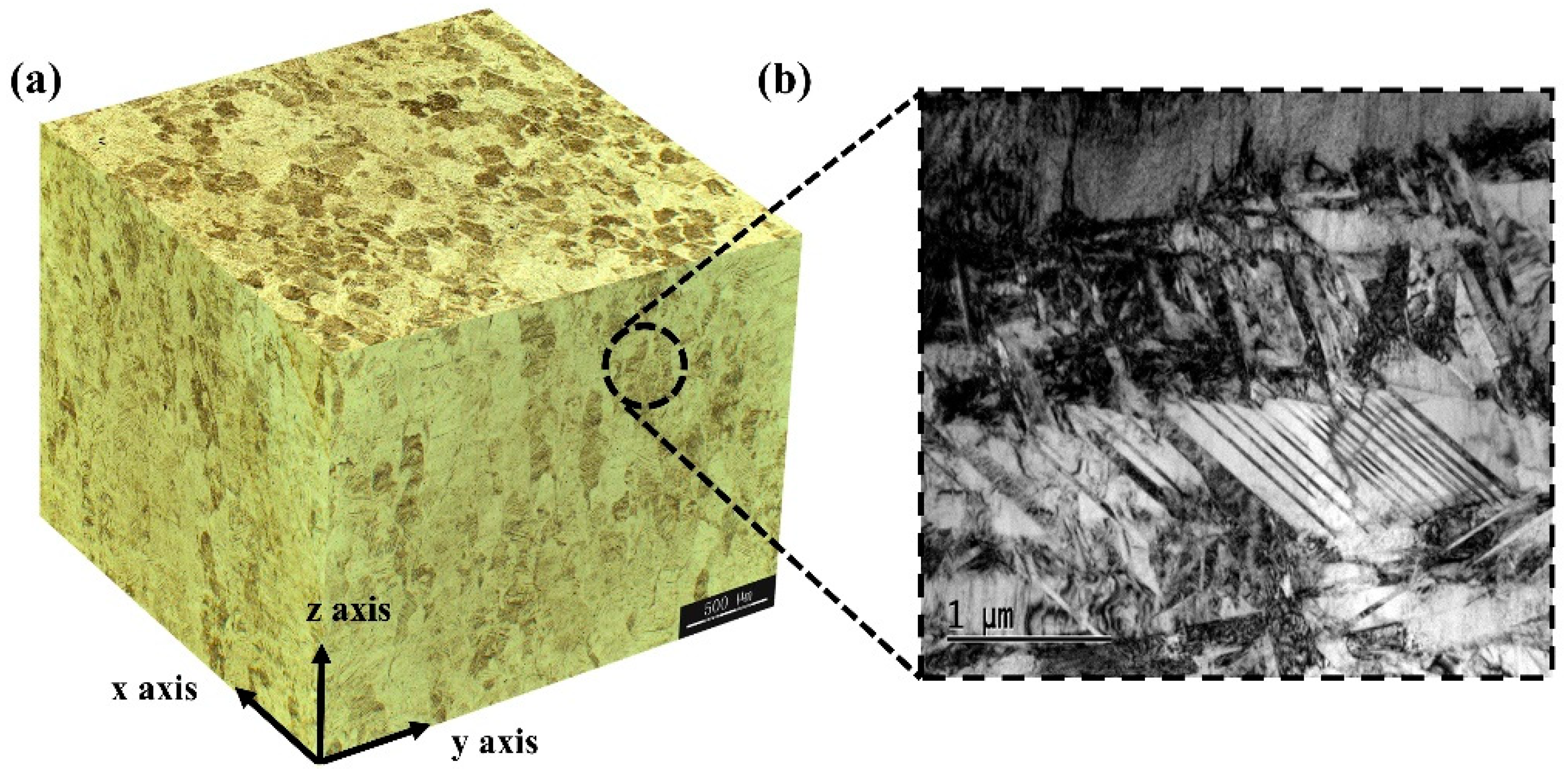
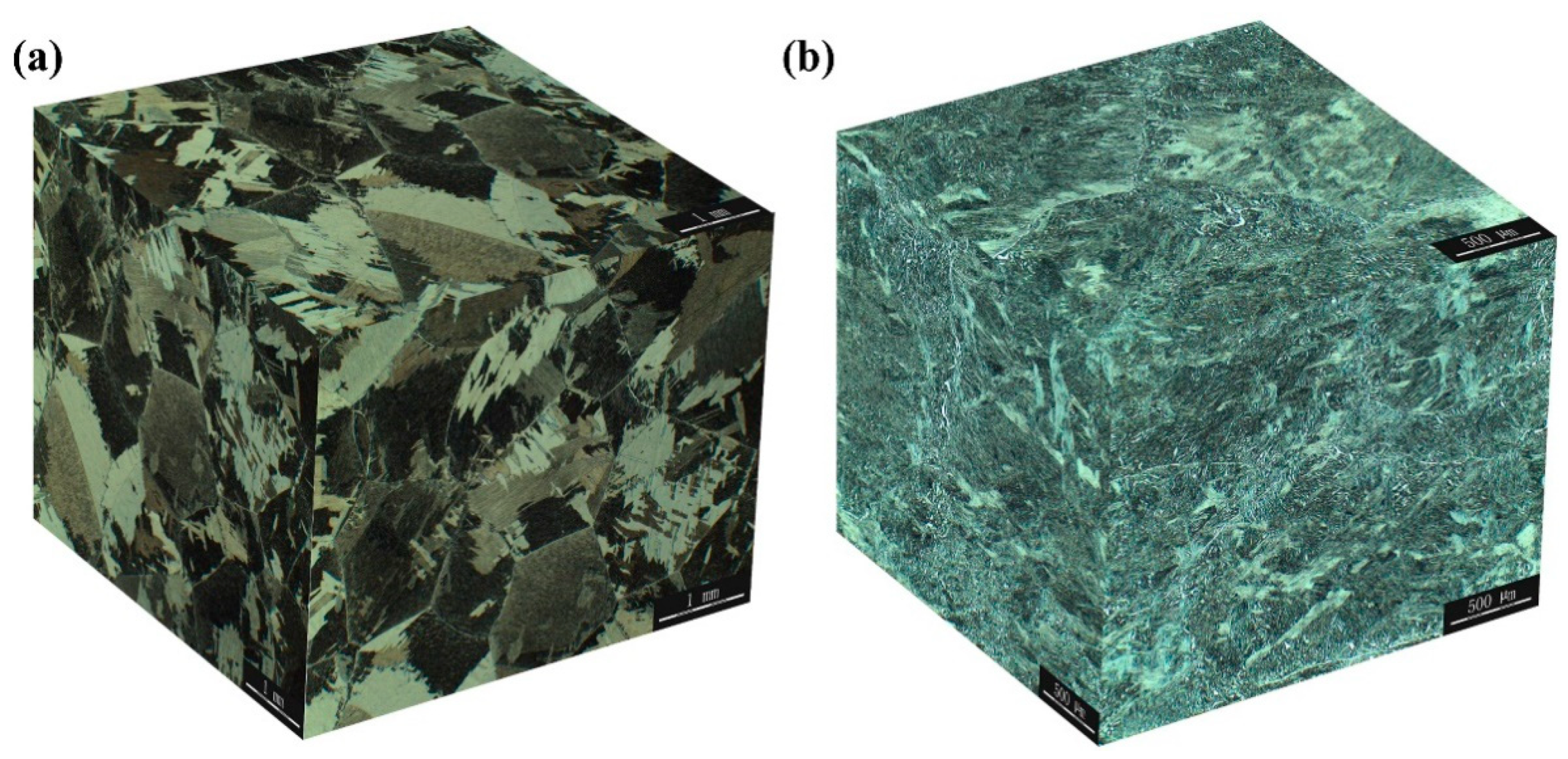
3.1. Microstructure and Properties of SLMed Ti–6Al–4V Alloy
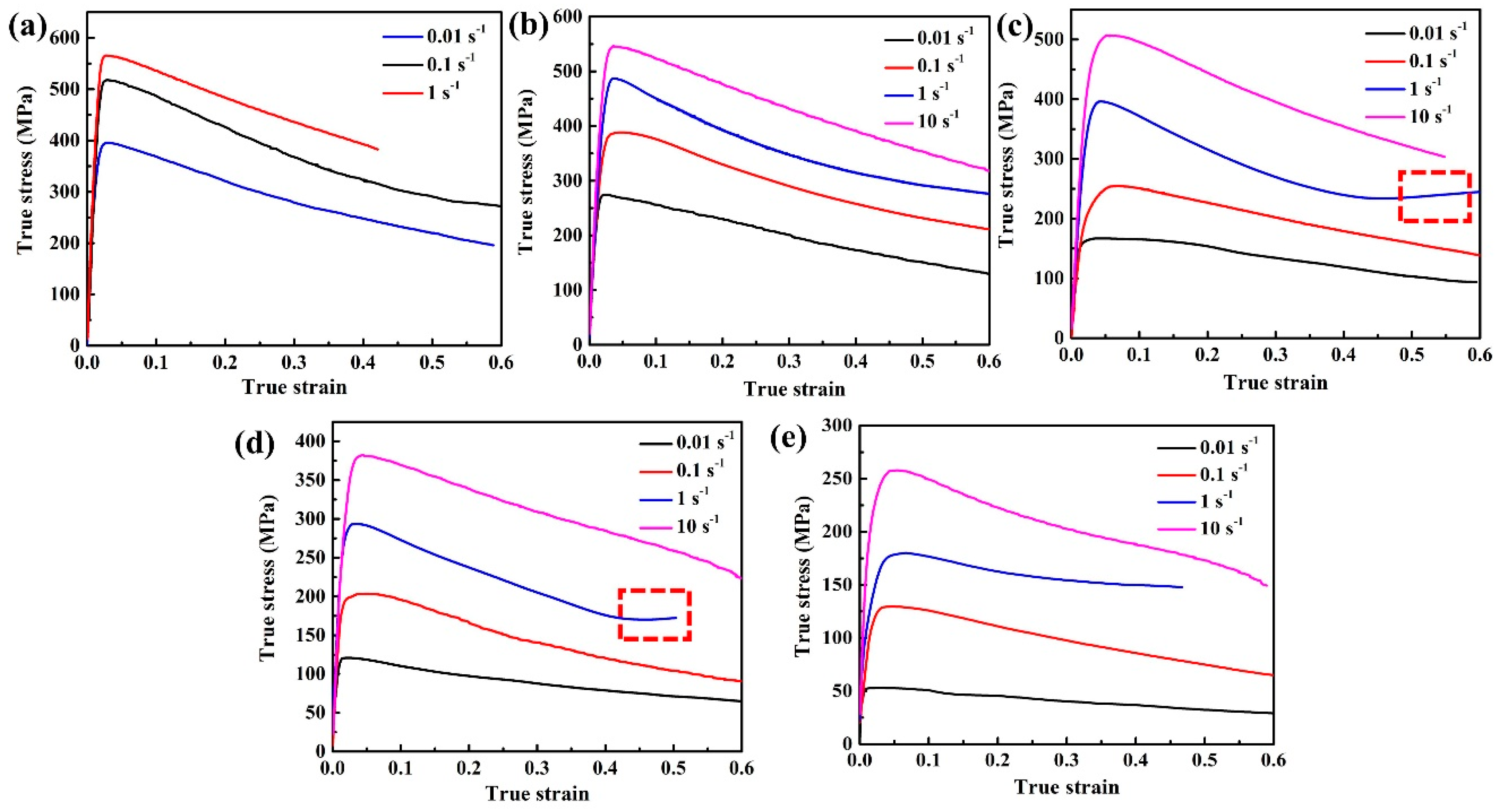
3.2. Flow Behavior
3.3. Constitutive Modeling
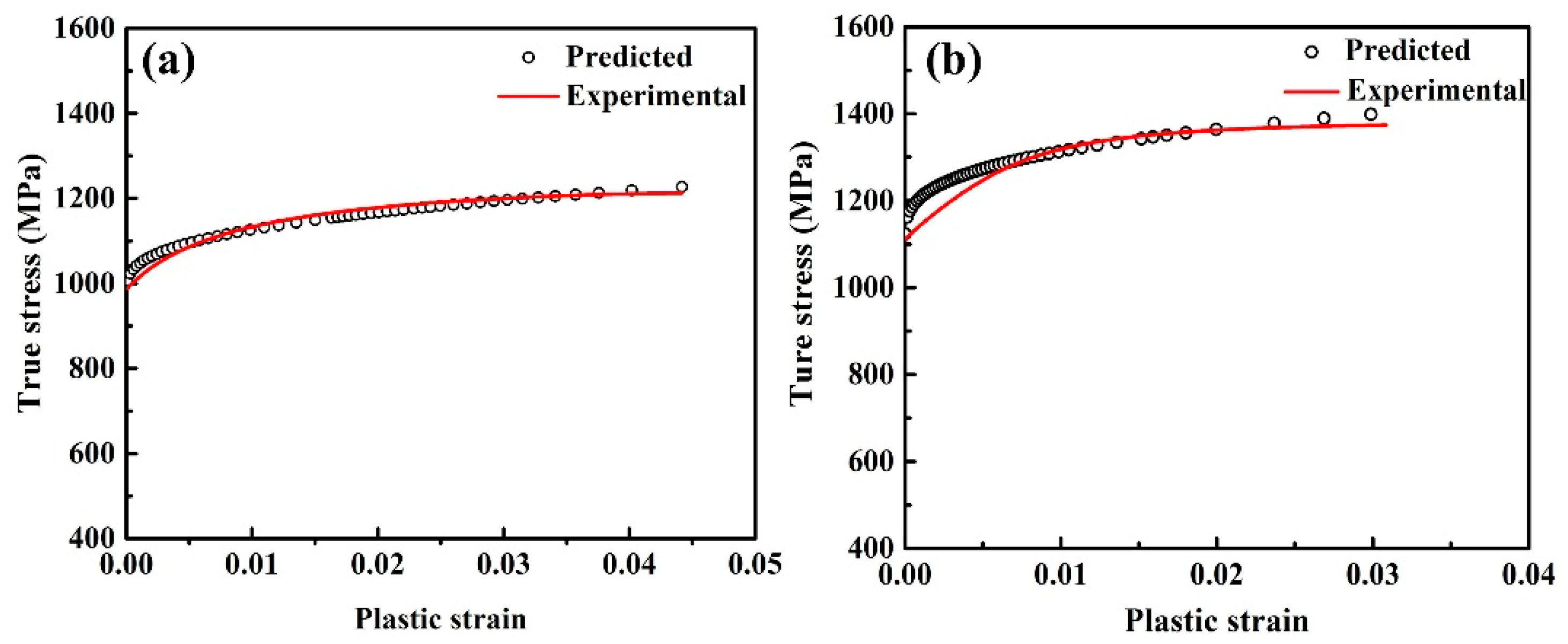
3.3.1. Quasi-Static Modeling
3.3.2. Dynamic Modeling
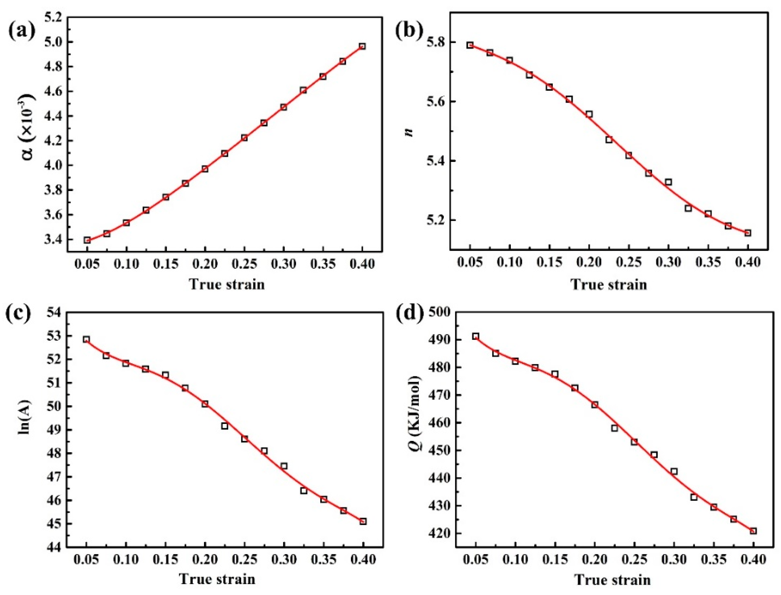
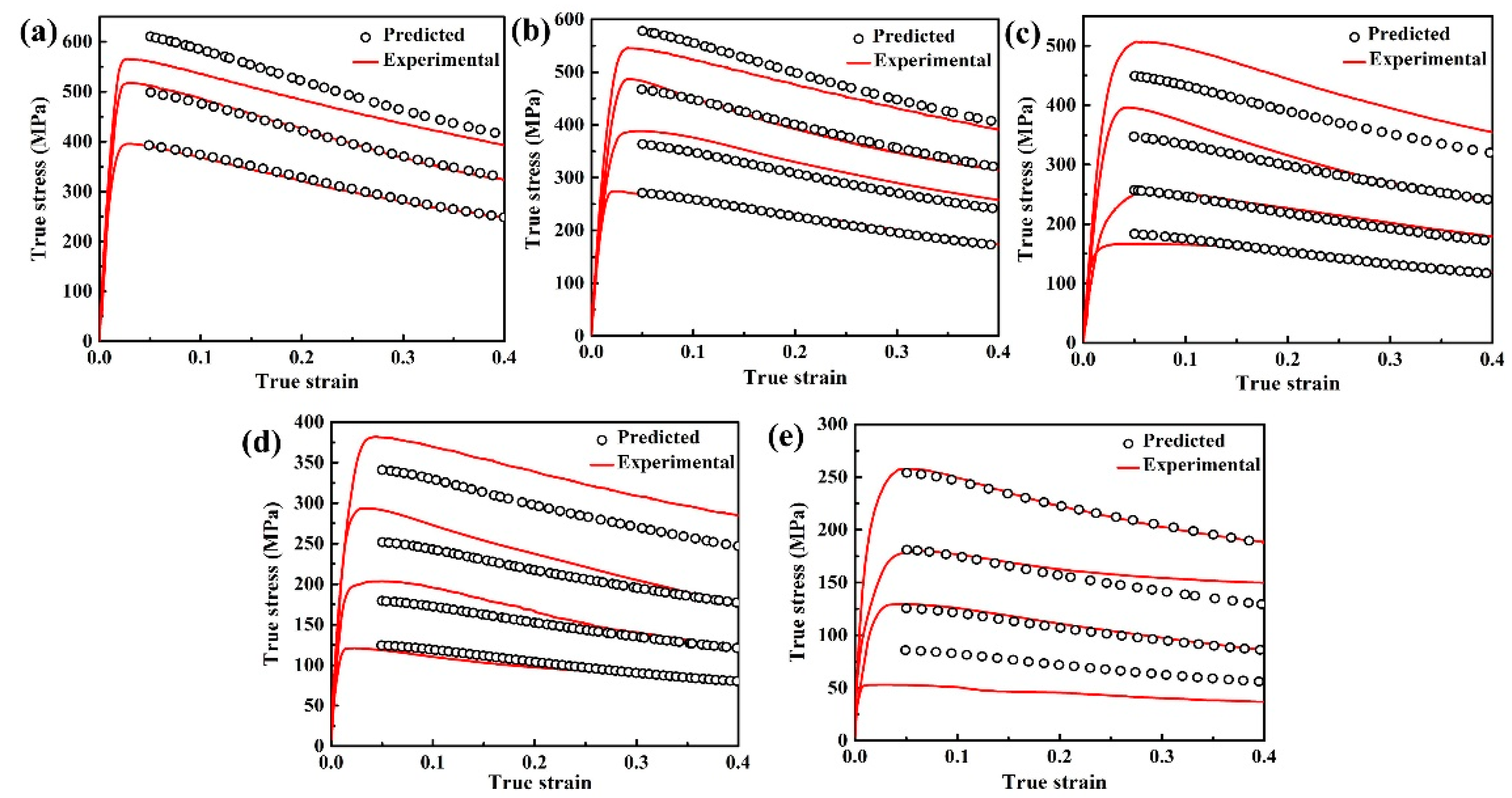
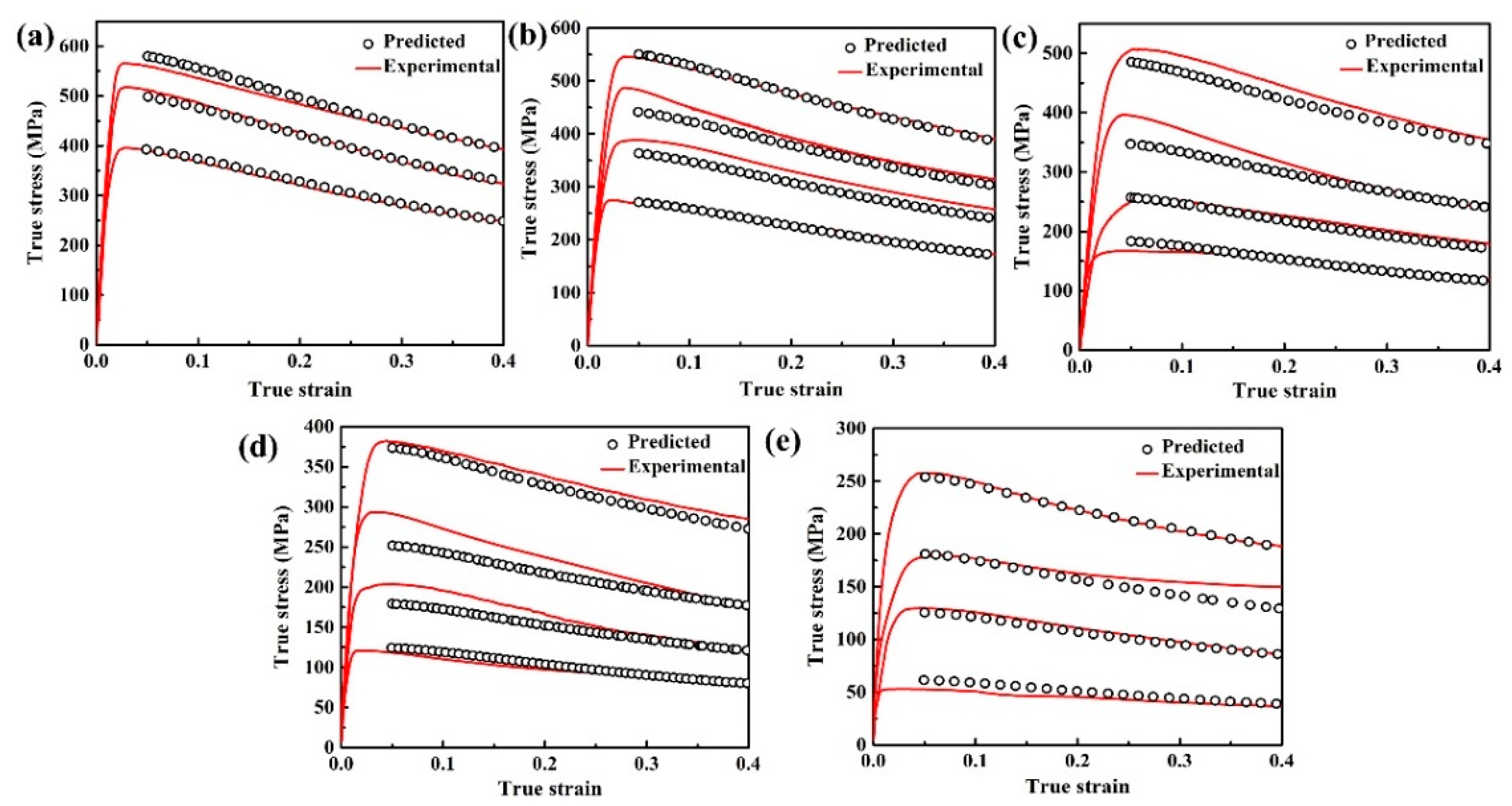
- The Arrhenius Model
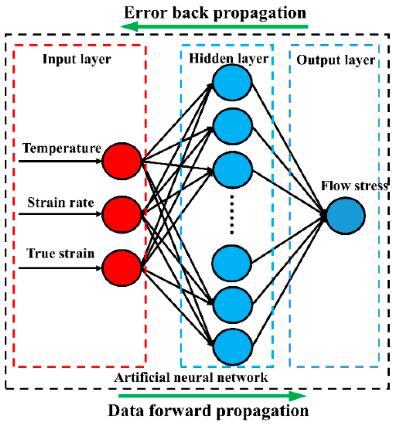
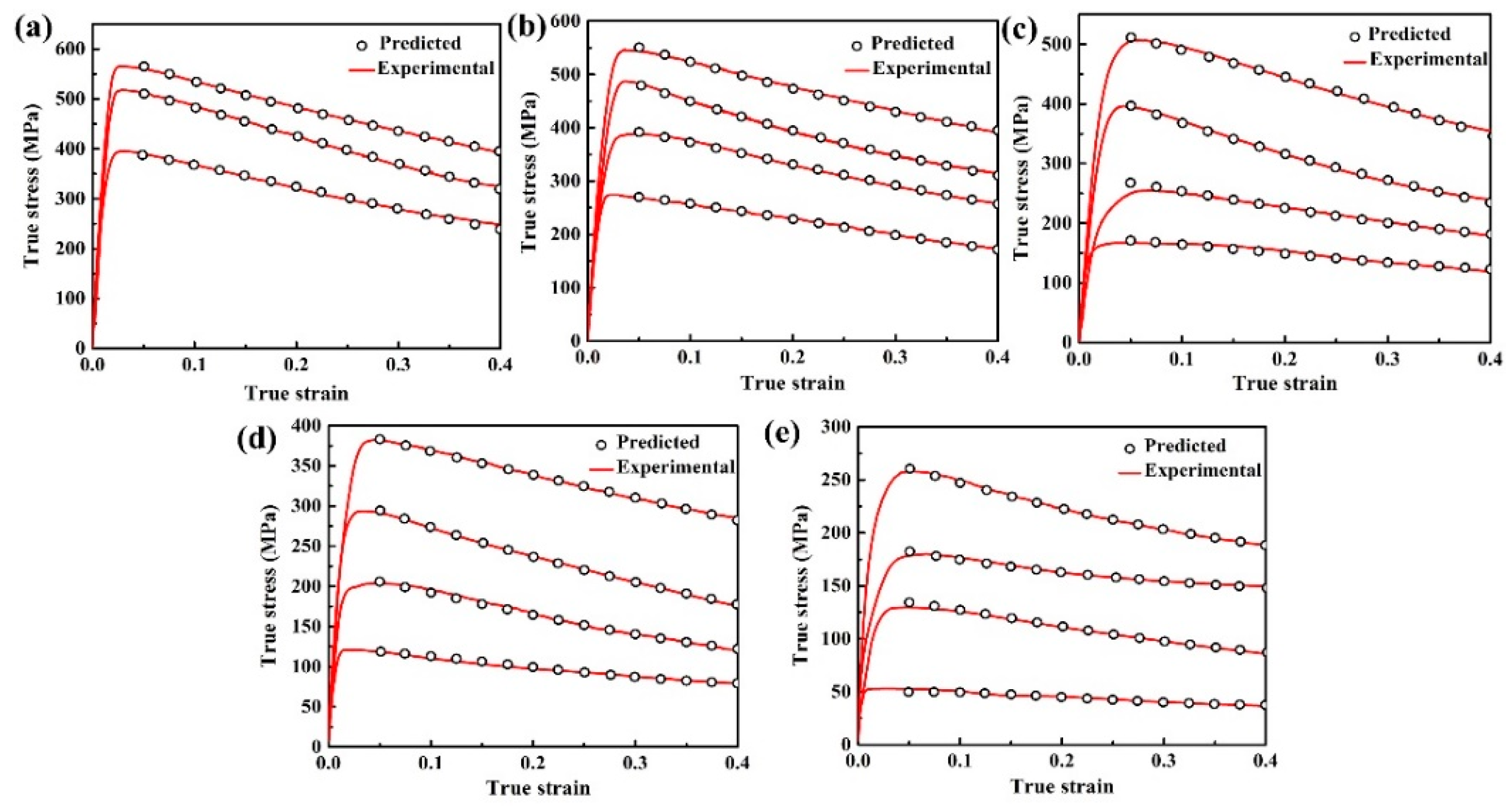
- The ANN Model
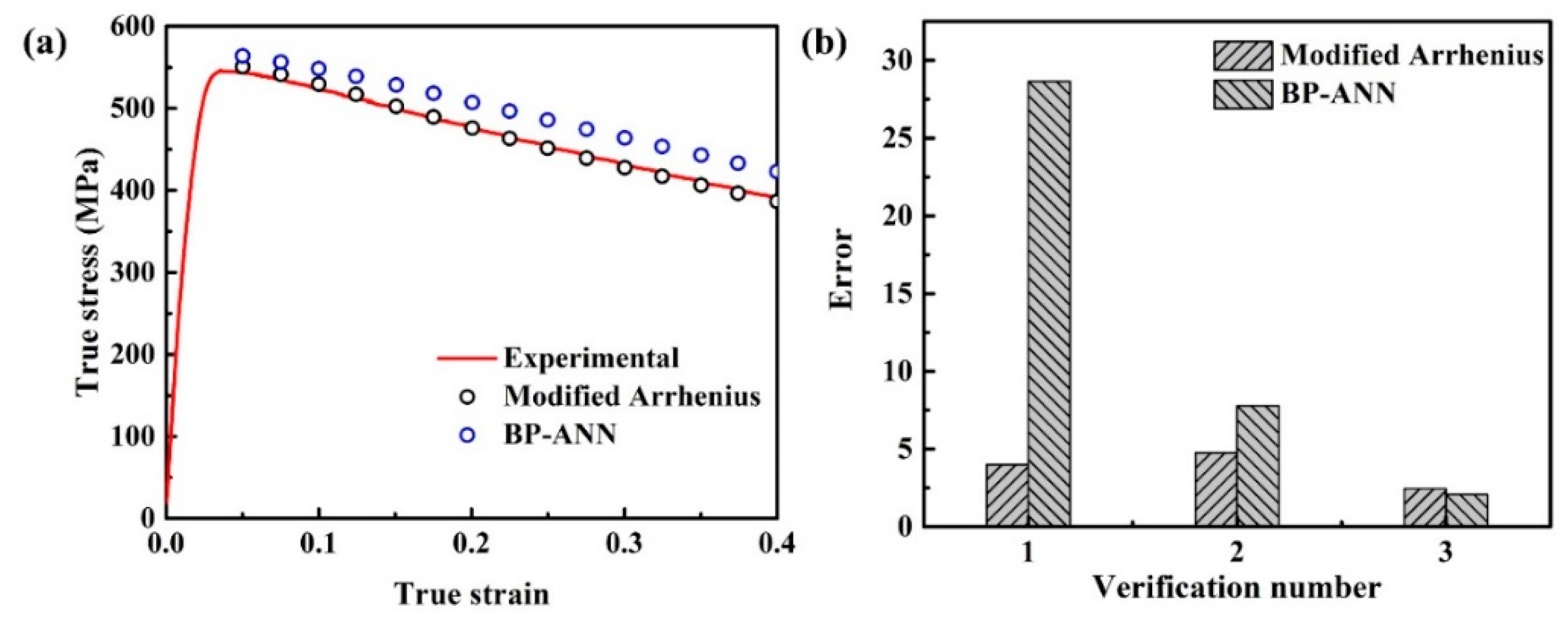
- Comparisons between the BP-ANN and the Modified Arrhenius Models
4. Conclusions
- (1)
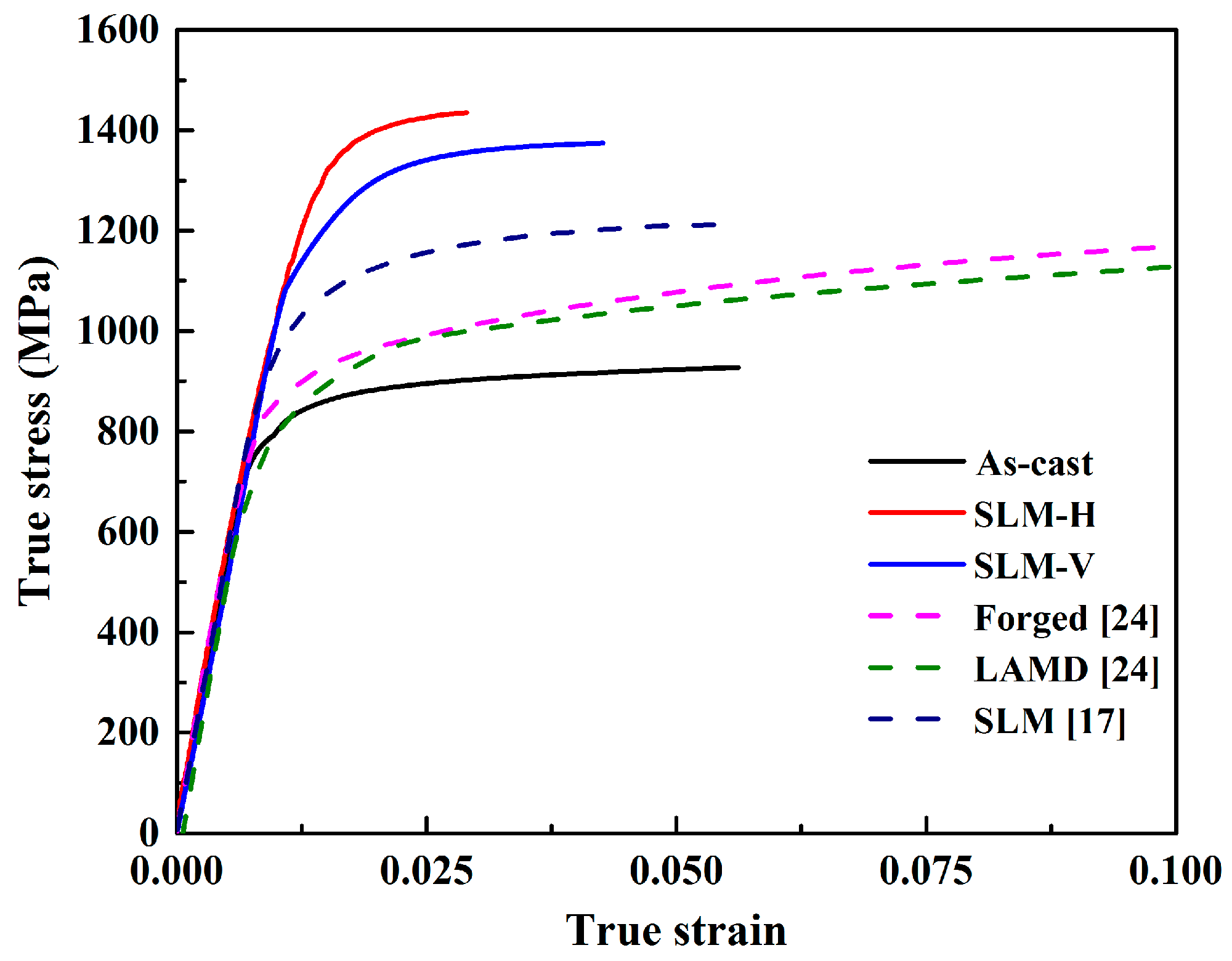
- The as-fabricated microstructure of Ti–6Al–4V alloy contains columnar grains and fine martensitic needles due to extremely fast cooling rates, resulting in higher strength and lower ductility at room temperature, compared to the as-cast and forged Ti–6Al–4V. The average yield and ultimate strength is as high as 1036–1187 MPa and about 1300 MPa, respectively. The average elongation to failure is 6.8–8.7% and the average reduction of area is 21.30–28.60%.
- (2)
- The room temperature quasi-static tensile behavior of the SLMed Ti–6Al–4V alloy exhibit the features of continuous yielding and unobvious work-hardening. During high-temperature dynamic compression, the flow stress quickly arrives at the peak value when the strain is small. The softening rate of flow stress varies with strain rates and temperatures.
- (3)
- The J–C model is suitable to forecast the quasi-static deformation behavior of SLMed Ti–6Al–4V at room temperature, but the model constants might rely on the specific process conditions because of the issue of building consistency.
- (4)
- The established modified Arrhenius and BP-ANN models could approach the stress-strain behavior during hot dynamic compression with enough precision. However, the established modified Arrhenius model is more predictive of the conditions out of the model data.
Author Contributions
Funding
Conflicts of Interest
References
- Tao, P.; Shao, H.; Ji, Z.; Nan, H.; Xu, Q. Numerical simulation for the investment casting process of a large-size titanium alloy thin-wall casing. Prog. Nat. Sci. 2018, 28, 520–528. [Google Scholar] [CrossRef]
- Banerjee, D.; Williams, J.C. Perspectives on titanium science and technology. Acta Mater. 2013, 61, 844–879. [Google Scholar] [CrossRef]
- Sallica-Leva, E.; Caram, R.; Jardini, A.L.; Fogagnolo, J.B. Ductility improvement due to martensite α′ decomposition in porous Ti–6Al–4V parts produced by selective laser melting for orthopedic implants. J. Mech. Behav. Biomed. Mater. 2016, 54, 149–158. [Google Scholar] [CrossRef] [PubMed]
- Chen, J.; Zhang, Z.; Chen, X.; Zhang, C.; Zhang, G.; Xu, Z. Design and manufacture of customized dental implants by using reverse engineering and selective laser melting technology. J. Prosthet. Dent. 2014, 112, 1088–1095. [Google Scholar] [CrossRef] [PubMed]
- Yan, C.; Hao, L.; Hussein, A.; Bubb, S.L.; Young, P.; Raymont, D. Evaluation of light-weight AlSi10Mg periodic cellular lattice structures fabricated via direct metal laser sintering. J. Mater. Process. Technol. 2014, 214, 856–864. [Google Scholar] [CrossRef]
- Herzog, D.; Seyda, V.; Wycisk, E.; Emmelmann, C. Additive manufacturing of metals. Acta Mater. 2016, 117, 371–392. [Google Scholar] [CrossRef]
- Sun, J.; Yang, Y.; Wang, D. Parametric optimization of selective laser melting for forming Ti6Al4V samples by Taguchi method. Opt. Laser Technol. 2013, 49, 118–124. [Google Scholar] [CrossRef]
- Yang, J.; Yu, H.; Yin, J.; Gao, M.; Wang, Z.; Zeng, X. Formation and control of martensite in Ti–6Al–4V alloy produced by selective laser melting. Mater. Des. 2016, 108, 308–318. [Google Scholar] [CrossRef]
- Simonelli, M.; Tse, Y.Y.; Tuck, C. Effect of the build orientation on the mechanical properties and fracture modes of SLM Ti–6Al–4V. Mater. Sci. Eng. A 2014, 616, 1–11. [Google Scholar] [CrossRef]
- Facchini, L.; Magalini, E.; Robotti, P.; Molinari, A.; Höges, S.; Wissenbach, K. Ductility of a Ti–6Al–4V alloy produced by selective laser melting of prealloyed powders. Rapid Prototyping J. 2010, 16, 450–459. [Google Scholar] [CrossRef]
- Edwards, P.; Ramulu, M. Fatigue performance evaluation of selective laser melted Ti–6Al–4V. Mater. Sci. Eng. A 2014, 598, 327–337. [Google Scholar] [CrossRef]
- Tao, P.; Li, H.-X.; Huang, B.-Y.; Hu, Q.-D.; Gong, S.-L.; Xu, Q.-Y. Tensile behavior of Ti–6Al–4V alloy fabricated by selective laser melting: Effects of microstructures and as-built surface quality. Chin. Foundry 2018, 15, 243–252. [Google Scholar] [CrossRef]
- Vilaro, T.; Colin, C.; Bartout, J.-D. As-fabricated and heat-treated microstructures of the Ti–6Al–4V alloy processed by selective laser melting. Metall. Mater. Trans. A 2011, 42, 3190–3199. [Google Scholar] [CrossRef]
- Kasperovich, G.; Hausmann, J. Improvement of fatigue resistance and ductility of TiAl6V4 processed by selective laser melting. J. Mater. Process. Technol. 2015, 220, 202–214. [Google Scholar] [CrossRef]
- Bagehorn, S.; Wehr, J.; Maier, H.J. Application of mechanical surface finishing processes for roughness reduction and fatigue improvement of additively manufactured Ti–6Al–4V parts. Int. J. Fatigue 2017, 102, 135–142. [Google Scholar] [CrossRef]
- Cheng, X.Y.; Li, S.J.; Murr, L.E.; Zhang, Z.B.; Hao, Y.L.; Yang, R.; Medina, F.; Wicker, R.B. Compression deformation behavior of Ti–6Al–4V alloy with cellular structures fabricated by electron beam melting. J. Mech. Behav. Biomed. Mater. 2012, 16, 153–162. [Google Scholar] [CrossRef] [PubMed]
- Gautam, R.; Idapalapati, S. Performance of strut-reinforced Kagome truss core structure under compression fabricated by selective laser melting. Mater. Des. 2019, 164, 107541. [Google Scholar] [CrossRef]
- Wang, Z.; Li, P. Characterisation and constitutive model of tensile properties of selective laser melted Ti–6Al–4V struts for microlattice structures. Mater. Sci. Eng. A 2018, 725, 350–358. [Google Scholar] [CrossRef]
- Baxter, C.; Cyr, E.; Odeshi, A.; Mohammadi, M. Constitutive models for the dynamic behaviour of direct metal laser sintered AlSi10Mg_200C under high strain rate shock loading. Mater. Sci. Eng. A 2018, 731, 296–308. [Google Scholar] [CrossRef]
- Lu, X.; Lin, X.; Chiumenti, M.; Cervera, M.; Li, J.; Ma, L.; Wei, L.; Hu, Y.; Huang, W. Finite element analysis and experimental validation of the thermomechanical behavior in laser solid forming of Ti–6Al–4V. Addit. Manuf. 2018, 21, 30–40. [Google Scholar] [CrossRef]
- Thijs, L.; Verhaeghe, F.; Craeghs, T.; Van Humbeeck, J.; Kruth, J.-P. A study of the microstructural evolution during selective laser melting of Ti–6Al–4V. Acta Mater. 2010, 58, 3303–3312. [Google Scholar] [CrossRef]
- Zhong, H.Z.; Zhang, X.Y.; Wang, S.X.; Gu, J.F. Examination of the twinning activity in additively manufactured Ti–6Al–4V. Mater. Des. 2018, 144, 14–24. [Google Scholar] [CrossRef]
- Åkerfeldt, P.; Antti, M.-L.; Pederson, R. Influence of microstructure on mechanical properties of laser metal wire-deposited Ti–6Al–4V. Mater. Sci. Eng. A 2016, 674, 428–437. [Google Scholar] [CrossRef]
- Li, P.-H.; Guo, W.-G.; Huang, W.-D.; Su, Y.; Lin, X.; Yuan, K.-B. Thermomechanical response of 3D laser-deposited Ti–6Al–4V alloy over a wide range of strain rates and temperatures. Mater. Sci. Eng. A 2015, 647, 34–42. [Google Scholar] [CrossRef]
- Matsumoto, H.; Bin, L.; Lee, S.-H.; Li, Y.; Ono, Y.; Chiba, A. Frequent Occurrence of Discontinuous Dynamic Recrystallization in Ti–6Al–4V Alloy with α′ Martensite Starting Microstructure. Metall. Mater. Trans. A 2013, 44, 3245–3260. [Google Scholar] [CrossRef]
- Mur, F.X.G.; Rodriguez, D.; Planell, J.A. Influence of tempering temperature and time on the α′-Ti–6Al–4V martensite. J. Alloys Compd. 1996, 234, 287–289. [Google Scholar]
- Zhang, Z.X.; Qu, S.J.; Feng, A.H.; Shen, J.; Chen, D.L. Hot deformation behavior of Ti–6Al–4V alloy: Effect of initial microstructure. J. Alloys Compd. 2017, 718, 170–181. [Google Scholar] [CrossRef]
- Lin, Y.C.; Chen, X.-M. A critical review of experimental results and constitutive descriptions for metals and alloys in hot working. Mater. Des. 2011, 32, 1733–1759. [Google Scholar] [CrossRef]
- Sellars, C.M.; McTegart, W.J. On the mechanism of hot deformation. Acta Metall. 1966, 14, 1136–1138. [Google Scholar] [CrossRef]
- Wang, J.; Zhao, G.; Chen, L.; Li, J. A comparative study of several constitutive models for powder metallurgy tungsten at elevated temperature. Mater. Des. 2016, 90, 91–100. [Google Scholar] [CrossRef]
- Li, J.; Li, F.; Cai, J.; Wang, R.; Yuan, Z.; Xue, F. Flow behavior modeling of the 7050 aluminum alloy at elevated temperatures considering the compensation of strain. Mater. Des. 2012, 42, 369–377. [Google Scholar] [CrossRef]
- Shafaat, M.A.; Omidvar, H.; Fallah, B. Prediction of hot compression flow curves of Ti–6Al–4V alloy in α + β phase region. Mater. Des. 2011, 32, 4689–4695. [Google Scholar] [CrossRef]
- Peng, X.; Guo, H.; Shi, Z.; Qin, C.; Zhao, Z. Constitutive equations for high temperature flow stress of TC4-DT alloy incorporating strain, strain rate and temperature. Mater. Des. 2013, 50, 198–206. [Google Scholar] [CrossRef]
- Wu, S.-W.; Zhou, X.-G.; Cao, G.-M.; Liu, Z.-Y.; Wang, G.-D. The improvement on constitutive modeling of Nb-Ti micro alloyed steel by using intelligent algorithms. Mater. Des. 2017, 116, 676–685. [Google Scholar] [CrossRef]
- Mosleh, A.; Mikhaylovskaya, A.; Kotov, A.; Pourcelot, T.; Aksenov, S.; Kwame, J.; Portnoy, V. Modelling of the superplastic deformation of the near-α titanium alloy (Ti-2.5 Al-1.8 Mn) using Arrhenius-type constitutive model and artificial neural network. Metals 2017, 7, 568. [Google Scholar] [CrossRef]


| Process | E (GPa) | σ0.2 (MPa) | σu (MPa) | EL (%) | R/A (%) |
|---|---|---|---|---|---|
| SLM-V | 115 ± 7.1 | 1036.70 ± 133.70 | 1309.50 ± 8.2 | 8.72 ± 2.77 | 28.60 ± 2.59 |
| SLM-H | 117 ± 2.2 | 1187.80 ± 35.84 | 1307.50 ± 7.4 | 6.80 ± 1.10 | 21.30 ± 1.66 |
| As-cast | 105.31 ± 9.2 | 776.54 ± 0.54 | 881.04 ± 2.22 | 12.78 ± 0.71 | 23.05 ± 4.2 |
| Forged | 112.53 ± 3.14 | 1023.50 ± 6.1 | 1037.30 ± 2.12 | 10.60 ± 0.63 | - |
| Process | A0 (MPa) | B (MPa) | n0 |
|---|---|---|---|
| SLM-V | 1100 | 889 | 0.32 |
| SLM-R | 980 | 735 | 0.34 |
| Process | AARE (%) | R |
|---|---|---|
| SLM-V | 2.5 | 0.98 |
| SLM-R | 1.1 | 0.99 |
| α | n | Q | lnA |
|---|---|---|---|
| d0 = 0.00336 | e0 = 5.8491 | f0 = 515,151.1705 | y0 = 55.5744 |
| d1 = −0.0011 | e1 = −1.5453 | f1 = −801,076.1344 | y1 = −91.6002 |
| d2 = 0.0400 | e2 = 11.9274 | f2 = 8,213,190.0000 | y2 = 941.9834 |
| d3 = −0.1386 | e3 = −106.1979 | f3 = −43,707,500.0000 | y3 = −5002.6724 |
| d4 = 0.2554 | e4 = 282.7306 | f4 = 99,228,900.0000 | y4 = 11362.8251 |
| d5 = −0.1969 | e5 = −236.7075 | f5 = −81,165,900.0000 | y5 = −9305.6516 |
| Model | AARE (%) | R |
|---|---|---|
| Arrhenius model | 7.6 | 0.987 |
| Modified Arrhenius model | 4.0 | 0.996 |
| BP-ANN model | 0.7 | 0.9998 |
| Verification Number | Temperature (°C) | Strain Rate (s−1) |
|---|---|---|
| No. 1 | 750 | 1 × 101 |
| No. 2 | 850 | 1 × 10⁻² |
| No. 3 | 900 | 1 × 10⁻¹ |
© 2019 by the authors. Licensee MDPI, Basel, Switzerland. This article is an open access article distributed under the terms and conditions of the Creative Commons Attribution (CC BY) license (http://creativecommons.org/licenses/by/4.0/).
Share and Cite
Tao, P.; Zhong, J.; Li, H.; Hu, Q.; Gong, S.; Xu, Q. Microstructure, Mechanical Properties, and Constitutive Models for Ti–6Al–4V Alloy Fabricated by Selective Laser Melting (SLM). Metals 2019, 9, 447. https://doi.org/10.3390/met9040447
Tao P, Zhong J, Li H, Hu Q, Gong S, Xu Q. Microstructure, Mechanical Properties, and Constitutive Models for Ti–6Al–4V Alloy Fabricated by Selective Laser Melting (SLM). Metals. 2019; 9(4):447. https://doi.org/10.3390/met9040447
Chicago/Turabian StyleTao, Pan, Jiangwei Zhong, Huaixue Li, Quandong Hu, Shuili Gong, and Qingyan Xu. 2019. "Microstructure, Mechanical Properties, and Constitutive Models for Ti–6Al–4V Alloy Fabricated by Selective Laser Melting (SLM)" Metals 9, no. 4: 447. https://doi.org/10.3390/met9040447
APA StyleTao, P., Zhong, J., Li, H., Hu, Q., Gong, S., & Xu, Q. (2019). Microstructure, Mechanical Properties, and Constitutive Models for Ti–6Al–4V Alloy Fabricated by Selective Laser Melting (SLM). Metals, 9(4), 447. https://doi.org/10.3390/met9040447