Abstract
In this paper, phase coherence imaging is proposed to improve spatial resolution and signal-to-noise ratio (SNR) of near-surface defects in rails using cross-correlation of ultrasonic diffuse fields. The direct signals acquired by the phased array are often obscured by nonlinear effects. Thus, the output image processed by conventional post-processing algorithms, like total focus method (TFM), has a blind zone close to the array. To overcome this problem, the diffuse fields, which contain spatial phase correlations, are applied to recover Green’s function. In addition, with the purpose of improving image quality, the Green’s function is further weighted by a special coherent factor, sign coherence factor (SCF), for grating and side lobes suppression. Experiments are conducted on two rails and data acquisition is completed by a commercial 32-element phased array. The quantitative performance comparison of TFM and SCF images is implemented in terms of the array performance indicator (API) and SNR. The results show that the API of SCF is significantly lower than that of TFM. As for SNR, SCF achieved a better SNR than that of TFM. The study in this paper provides an experimental reference for detecting near-surface defects in the rails.
1. Introduction
The defect detection of rails means a great deal to the safe operation of the railway system and industrial applications. Corrosions, cracks, and cavities in rails not only shorten the life of the railway services but also lead to potential security risks. Therefore, it is of great significance to pursue structural health monitoring (SHM) of rails. As one of the popular SHM technologies, ultrasonic phased array has been developed and widely used in recent years. By exciting the array elements in a specified sequence, one array probe can steer and focus the wavefront into a structure, allowing the generation of structure images [1]. However, in practice, there is always a blind zone immediately in front of the inspection system and it extends to several millimeters in common engineering. This causes the direct arrival of ultrasonic phased arrays containing the undesired signals, where early detection of signals will be obscured [2].
A promising method to solve this problem is the cross-correlation of diffuse fields. This approach can retrieve Green’s function between two points from a diffuse field. In 1999, Claerbout et al. [3] proposed a hypothesis that cross-correlation of seismic traces formed by randomly distributed deep seismic sources can generate virtual ground seismic records. A coherent wave field was constructed by calculating the cross-correlation of noise recorded at two locations on the surface. In 2001, Weaver et al. [4] validated that the impulse response of the structure between two receiving points can be extracted by using the cross-correlation of noise recorded at two receiving points in random noise fields. The retrieved signals were only different in magnitude from Green’s function. From then on, due to the ability of retrieving deterministic signals (Green’s function) from random signals, this method has been applied in many fields, such as electromagnetics [5], seismology [6,7], ocean acoustics [8], civil engineering [9], medicine [10], and ultrasonics [11]. In 2004, under the isotropic scattering assumption, Snieder et al. [12] deduced the feasibility of recovering Green’s function of the ballistic wave from the coda. The global requirement of the equipartitioning of normal modes was held if the scattered waves propagated quasi-isotropically near the receivers. Subsequently, after considering the limitation of time-reversal invariance in correlating noise, he found that it was possible to obtain Green’s function of diffusion by correlating the solutions of the diffusion equation that were excited randomly [13]. This property was used to retrieve Green’s function for diffusive systems from ambient fluctuations. In 2011, Moulin et al. [14] tested ambient vibrations for passive real-time monitoring of structures by low-frequency random vibration data, which was collected on an all-aluminum naval vessel operating at high speed. In 2014, Roux et al. [15] evaluated the relative contributions of source distribution and medium complexity in the two-point cross-correlations, showing that the fit between the cross-correlation and the 2D Green’s function strongly depended on the nature of the excitation source. In 2015, Chehami et al. [16] applied passive listening to monitor the occurrence of defects in thin aluminum plates. The defects were localized successfully from noise generated by different sources between 10 and 40 kHz in metallic plates. In 2017, with the experiment on both aluminum and CRFP blocks, Potter et al. [2] showed that a reconstructed full matrix which contained the near-surface information can be produced through cross-correlation of a diffuse full matrix.
The total focusing method (TFM) is a traditional post-processing imaging algorithm for phased array and shows great potential in defect detection and characterization. It was introduced by Holmes [17] in 2005. TFM utilizes all possible combinations of sending and receiving elements to form an image. Compared to the other imaging methods, for example, the B-scan mode (whose image is constructed line by line and by focusing at a given depth), the TFM allows to focus on every point of the image area. TFM is considered the “gold standard” that provides high resolution and a larger dynamic range. However, because there is only one element used at every emission, the energy sent into the medium is limited. Thus, the signal-to-noise ratio (SNR) of TFM is low compared to equivalent imaging implemented using conventional parallel transmit beam-forming. In addition, the image artifacts of TFM will lead to misinterpretations, which may ultimately cause low image quality.
Recently, a novel method, phase coherent imaging, has been proposed to improve the quality of ultrasound images [18]. Based on a statistical analysis of the instantaneous phase of the aperture data, a phase coherence factor is computed for every sampling point. If all echoes are from the focal region, they overlap perfectly after inserting the beam-forming delays and the variance of their phases is close to zero. The echo signal can be kept in the output image as the coherence factor is unity. On the other hand, if the echoes come from noise, the variance of their phases is non-zero. The coherence factor greatly reduces the noise amplitude in the output image. In order to simplify the implementation of this technique, the sign bit of the digitized received echo can be considered as a representative of the instantaneous phase. The sign coherence factor (SCF), a special phase coherence factor, can be obtained from the variance of the sign bit. It has been demonstrated that SCF simultaneously reduces undesirable echoes and the main lobe width. In this work, the application of SCF to increase spatial resolution and SNR for near-surface imaging in rails is investigated. The theoretical background of the work is presented first. Then, experiments are conducted in rails with a linear 32-element phased array. To recover near-surface information, Green’s function is retrieved from the cross-correlation of a diffuse full matrix. The output images are formed by TFM and SCF using Green’s function. Finally, the performance of the two algorithms for the near-surface defect is compared and conclusions are presented.
This paper is organized with seven sections, including this introduction. Section 2 demonstrates the theoretical background of this work. Section 3 presents the experimental apparatus for near-surface detection. Experimental results are illustrated in Section 4. Section 5 compares the performance of TFM and SCF algorithms in terms of array performance indicator (API) and SNR. Section 6 provides a recommendation for future research. Section 7 makes a conclusion of the findings.
2. Theoretical Background
2.1. The Theory of Diffuse Fields
The noise, caused by material backscattered energy correlated over time, is always considered the limiting factor in most ultrasonic defect detection scenarios [19]. It resists detailed analysis and should be eliminated to yield quality results. However, for multiple scattering and reflection effects, the randomization of elastic energy favors the formation of diffuse fields over long reverberation times, especially when the structure is complex. Thus, the non-stationary noise can be processed as a passive means to estimate Green’s function by cross-correlation.
In fact, the strong correlation of fields generated by different non-correlated sources in time and space is the result of wave propagation. Although the wave fields generated by random sources are not correlated with each other, the signals received by the two sensors from the same random source are correlated. The relationship between the cross-correlation and Green’s function recovery theory can be established by different methods, such as time reversal [20], diffusion [21], stationary phase [12], reciprocity theories [20], and modal equipartition [22]. The above methods proved that the time derivative of the cross-correlation of diffuse fields between two points is proportional to the difference between the causal Green’s function and the anti-causal Green’s function.
Figure 1 shows the schematic diagram of the rail. For a linear phased array, the linear distribution of elements causes the non-uniformity of the diffusion field in the test structure, which leads to the imperfect extraction of the diffusion field signals. In an ideal case, the diffuse field is formed by thermal fluctuations and the energy distribution of which is uniform. However, the reality is, the noise sources have a band-limited spectrum and their distribution is not always uniform in space and time [23]. The energy loss is inevitable in the structure and the receiving elements of the phased array have their own transducer response characteristics. In this paper, rather than the time derivative of the cross-correlation of the diffuse field, the averaged cross-correlation of the diffuse field is used for detecting defects. This is because a non-ideal environment is created by a finite number of sources having imperfect uniform distributions to simulate a realistic structure [24].
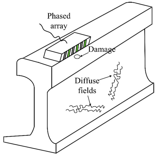
Figure 1.
Schematic diagram of the data acquisition system.
2.2. Green’s Function Reconstruction
The full matrix capture, which records time-domain signals from each transmitter-receiver element pair, can acquire a complete set of time-domain signals termed as a full matrix. The conventional full matrix is always applied to interrogate the structure and can be denoted as hi,j(t), where i denotes the transmitting element and j denotes the receiving element. Similarly, the diffuse full matrix di,j(t) is recorded after a long time of transmission tr. Then, a reconstructed full matrix gi,j(t) is built from di,j(t) by cross-correlating the responses of element i with that of element j, averaged over all transmitting elements [5]. It is written as follows:
where T is the window length and N is the total number of phased array elements. It is found that the larger the window length T, the more the coherent signals are recovered. In practice, the recovery of Green’s functions within the reconstructed full matrix is less accurate than directly acquired signals. The response from the interior of the part is better acquired from conventional capture while near-surface information is obtained more accurately using reconstruction. Therefore, the hybrid full matrix is introduced:
where the parameter tc is the time immediately after the effects of saturation have disappeared from the conventional full matrix. The parameter α determines the transition of the hybrid matrix. The parameter tb denotes the time of first back wall reflection. Parameter β is the scaling factor to normalize amplitude before summation to form the hybrid full matrix.
2.3. Imaging Technique
2.3.1. TFM Imaging
The TFM imaging is equivalent to a dynamic focusing in transmission and receiving modes at every point of a region of interest [17]. This algorithm generates a scalar function of position in the test structure and the amplitude of which can be represented as an image. Throughout this paper, the Cartesian co-ordinate system is used. The equi-spaced elements are relatively long in the y-direction and the propagation of energy is only in the X-Z plane. A two-dimensional model can be established for the transducer, as shown in Figure 2. For a linear array of N elements and time domain data Sij from all transmitter i and receiver j combinations, the image value at point (x, z) can be obtained:
where xi and xj are the position of transmitter and receiver on the X-axis.
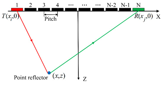
Figure 2.
Schematic diagram of total focus method (TFM).
2.3.2. SCF Imaging
SCF is applied to weight the coherent sum output and shows a high degree of robustness to noise. It uses phase rather than amplitude information to form an output image [18]. The output image is based on phase variance at the aperture data and can focus synthetically at every image pixel, which is computed as
SCFi is a weighting factor expressed as
although it has been shown that different p values can result in increased grating lobe suppression, for simplicity we set p = 1 in this paper. bij is the polarity of the aperture data:
If all of the received echoes are in phase at the focal point, which is corresponding to all of bij(t) have the same polarity, the weighting factor SCF is maximum and equal to one. Conversely, if half of the aperture data are positive and the other half negative, SCF is minimum and equal to zero. In other cases, the value of SCF is in the range [0, 1]. It has been shown that SCF can suppress the grating and side lobe and simultaneously increase the resolution. Based on an analysis of phase distribution in the aperture data, SCF also improves SNR [18].
3. Experimental Setup
An experimental system was designed and built as shown in Figure 3. The commercial phased array controller (Multi2000, M2M Inc., Les Ulis, France) was connected to a standard desktop PC, allowing capture of all pulse-echo and independent pitch-catch signals for offline post-processing. Specific information about the controller can be found in Table 1. The linear array used for the experiments was one-dimensional and consisted of 32 piezoelectric elements with 1 mm pitch, 0.1 mm inter-element spacing, and 5 MHz center frequency. The specimens were U71Mn hot-rolled rails.
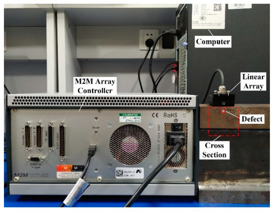
Figure 3.
Schematic diagram of the data acquisition system.

Table 1.
Array controller settings.
The array probe was placed on the top surface with direct contact in the experiments and two-dimensional images were produced in the X-Z plane. Both specimens were 290 mm in length and 174 mm in height. Figure 4 presented the cross-section of specimens in Figure 3. The coordinate origin was at the center of the array, on the material surface. For specimen 1, the diameter of the artificial hole was 6 mm and the position was x = 0 mm, z = 8 mm with respect to the array center, as shown in Figure 4a. For specimen 2, the diameters of the four defects were all 3 mm. The horizontal positions (X-axis) of all defects were 0 mm, the vertical positions (Z-axis) from the center of the array were 8 mm, 19 mm, 29 mm, and 39 mm, respectively, as shown in Figure 4b.
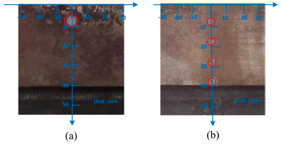
Figure 4.
Cross-section of rails: (a) Specimen 1; (b) Specimen 2.
When a transducer radiates into an isotropic solid half-space, the beam-pattern is complicated, including both longitudinal and shear wave modes. For simplicity, shear waves will be ignored [25]. In order to reduce the influence of noise, we filtered the raw acquisition data in a pre-processing stage to extract the scattered longitudinal wave signals. The offline post-processing algorithm was executed by MATLAB (The MathWorks Inc., Natick, MA, USA). We set tr = 600 μs and T = 100 μs for both cases. The velocity of the bulk longitudinal wave was approximately 5900 m·s−1. The flow chart of the experimental procedure is shown in Figure 5.
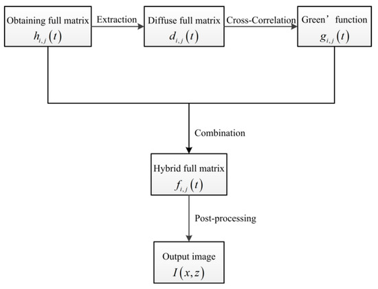
Figure 5.
Flow chart of the experimental procedure.
4. Experimental Results
4.1. The Reconstructed Green’s Function
An example of time traces in specimen 1 for i = j = 16 is presented in Figure 6. Every time trace was normalized to its maximum amplitude. Figure 6a shows the time trace of the conventional full matrix where nonlinear effects were observed between 0 and 2 μs. It was easy to conclude that the parameter tc was 2 μs. Furthermore, what can be seen clearly from Figure 6a was that the time to the first back wall tb was 59 μs. The signal of the diffuse full matrix was apparently random noise and no details about the test structure were given, as shown in Figure 6b. However, valuable information could be deduced from random noise. By the cross-correlation of the diffuse full matrix, Green’s function containing structure information was retrieved in Figure 6c. The causal part of Green’s function was the reconstructed full matrix gi,j(t). In Figure 6d, it became apparent that nonlinear effects no longer existed in a hybrid full matrix and the early time information could be observed visually with α = 20 × 106 s−1. This established the basis for near-surface imaging.
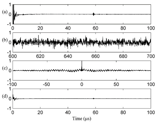
Figure 6.
Time traces for i = j = 16 in specimen 1: (a) Conventional full matrix; (b) diffuse full matrix; (c) Green’s function; (d) hybrid full matrix.
4.2. Imaging Results for Near-Surface Defects
The imaging results of the two specimens are shown in Figure 7 and Figure 8. The dimensions (x × z) of the image were 200 × 300 pixels, and the pixel dimensions were 0.15 × 0.17 mm. Obviously, the near-surface defect was masked and the image quality was low in Figure 7a,d and Figure 8a,d. This is because the conventional full matrix was affected by nonlinear effects, as mentioned before. The early time information was recovered from the cross-correlation of the diffuse full matrix, thus the hybrid full matrix contained the near-surface defect signals. Consequently, the near-surface imaging for specimen 1 was realized in Figure 7b,e. In the meantime, because the use of the hybrid full matrix, near-surface and bulk imaging for specimen 2 was achieved, as shown in Figure 8b,e. Although the near-surface defect became obvious compared with traditional inspection, the quality of TFM images still needed to be further strengthened for better visualization. In Figure 7c,f and Figure 8c,f, SCF improved the contrast and reduced artifacts, side and grating lobes effects. When compared to the imaging results of TFM, the defects were more clearly identified.
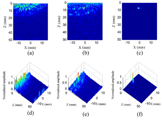
Figure 7.
The images for specimen 1: (a,d) TFM with conventional full matrix; (b,e) TFM with hybrid full matrix; (c,f) sign coherence factor (SCF) with hybrid full matrix.
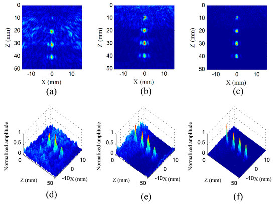
Figure 8.
The images for specimen 2: (a,d) TFM with conventional full matrix; (b,e) TFM with hybrid full matrix; (c,f) SCF with hybrid full matrix.
5. Analysis and Discussions
Close to the array, there is a strong blind zone, which is a region with high intensity artifacts. The near-surface defects cannot be shown by the conventional TFM method. On the one hand, the direct arrivals of phased arrays are characterized by the limited time associated with the conversion from the transmission to the reception operation, as well as the saturation from the transmission of the initial activation and the nonlinear electronic recovery process. On the other hand, the adjacent elements of phased arrays cause electrical and mechanical cross-talk, which also brings nonlinear effects into an early acoustic time of signals. In addition, the time of flight of the direct propagation and multiple reflections between the elements is short when compared to the echoes coming from the defects. Therefore, it reduces defect contrasts and masks defects located close to the array. The blind zone is pronounced in TFM image. To overcome this limitation, the Green’s function is recovered from the cross-correlation of the diffuse field. It makes near-surface imaging possible for post-processing algorithms, as shown in Figure 7 and Figure 8. Besides, the image processed by SCF will have better quality. Pixels in the TFM image are summed by the amplitude of signals, which is easily affected by noise. In SCF image, pixels corresponding to reflections from the main lobe are strongly weighted whereas those corresponding to grating lobe reflections have a low weight. This technique would improve spatial resolution and SNR.
Figure 9 shows the effect of different α for specimen 2 imaging. The first line is TFM images and the second line is SCF images. The parameter α determines the transition of the output image. The low α, whose value is 20 × 105 s−1, has a smooth transition in Figure 9a. However, more noise in the diffuse full matrix will be brought into the TFM image in the depth of about 20 mm to 50 mm. In Figure 9b, a relatively higher value of the parameter α, which is 20 × 106 s−1, is presented for imaging. Compared with Figure 9a, the noise is suppressed, and the image quality is improved. Another noteworthy feature is that there is a discontinuity at a depth of about 20 mm. Actually, considering the early time information and the later time information of the hybrid full matrix that come from conventional and reconstructed matrices, respectively, the data of the two matrices is different and the perfect combination of them can be hard to achieve, especially when defects are at different depths. To the authors’ knowledge, there is no algorithm or method that can determine the right value of parameter α. Therefore, suggesting an exact α is difficult in practice but we recommend that the range should be in [105, 107]. Beyond this range, the image quality will be degraded, even when the output image is weighted by SCF. In Figure 9c,d, contrary to TFM images, SCF images present good robustness to noise and keeps a high value of SNR to different α. What’s more, due to the reduction of grating lobe artifacts, all target defects remain visible and SCF images are not disturbed by discontinuity.
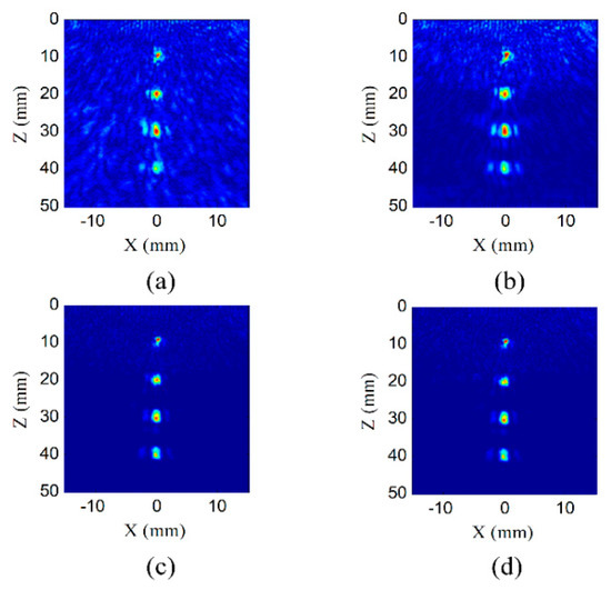
Figure 9.
TFM images for (a) α = 20 × 105 s−1, (b) α = 20 × 106 s−1; SCF images for (c) α = 20 × 105 s−1, (d) α = 20 × 106 s−1.
In order to quantitatively compare the performance of TFM and SCF imaging methods for near-surface point-like defects, the API and SNR are calculated. They are expressed by the following equations:
where A is the area over which the amplitude of the point-spread function (i.e., the image of an omnidirectional point scatterer) is greater than some threshold below its maximum value and λ is the wavelength at the center frequency. The API is a dimensionless quantity that represents the spatial extent of the point-spread function. Therefore, the function p depends on the imaging point and the threshold value. Note that a low value of API is desirable.
where Imax is the maximum value of the defect signal and Iaverage is the average amplitude of the background noise level.
A rectangular region (from −7.5 to 7.5 mm in the X-axis, from 0 to 15 mm in the Z-axis) of specimen 1 is shown in Figure 10. The image of TFM in Figure 10a,b and that of SCF in Figure 10d,e are presented. In Figure 10a,b, the noise emerges dramatically near the surface and side lobes exist in the TFM images. Artifacts with different degrees occurred with the TFM and degraded the image quality. However, with the usage of the SCF, the output images have the ability to suppress side lobes and grating lobes, as shown in Figure 10d,e. Figure 10c,f demonstrate the corresponding point-spread functions. In Figure 10c, noise is obviously observed at a depth of around 0 mm to 15 mm and the areas over the amplitude at −6 dB are 75.55 mm2, which are more than the areas of real defects in specimen 2. Furthermore, the side lobes result in misinterpretations of the defect. On the contrary, in Figure 10f, noise is effectively suppressed. The areas over the amplitude of −6 dB are all in the defect region and the side lobes are not present. This shows that SCF realizes better spatial resolution than TFM with data originating from diffuse fields. Another rectangular region (from −9 to 9 mm in the X-axis, from 0 to 45 mm in the Z-axis) of specimen 2 and the corresponding point-spread functions are shown in Figure 11.
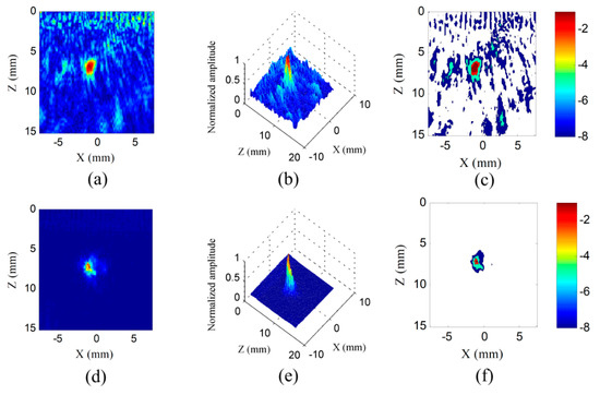
Figure 10.
The hybrid full matrix of specimen 1 processed by (a,b) TFM and (d,e) SCF. Corresponding point-spread functions: (c) TFM and (f) SCF.
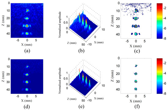
Figure 11.
The hybrid full matrix of specimen 2 processed by (a,b) TFM and (d,e) SCF. Corresponding point-spread functions: (c) TFM and (f) SCF.
To further illustrate the advantage of SCF, Figure 12 investigates the dependence of the API on different threshold values of the defect located at the same depth z = 8 mm. The range of threshold values are −10 to −1 dB. There is a significant difference in the API between TFM and SCF. In both cases, APIs for SCF remain stable at a low level. Alternatively, for lower thresholds, the APIs corresponding to the TFM increases much faster than APIs for SCF, especially for threshold values less than −4 dB. The APIs of TFM on low threshold values are unusually high and they are caused by noise. As for near-surface imaging in this paper, the noise comes not only from the diffuse scattering medium but also from the imperfect reconstruction of Green’s function. In fact, there is no formal guarantee that the noise cross-correlation function would yield an unbiased estimate of the full Green’s function. Thus, the amplitude distribution of the extracted coherent signals from the cross-correlation function is different from the amplitude distribution of the arrivals of the actual Green’s function. Moreover, for the limited number of averaging operations, the recovery of Green’s functions within the reconstructed full matrix is less accurate than directly acquired signals.
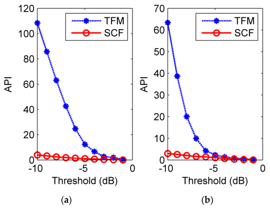
Figure 12.
The dependence of the array performance indicator (API) on the different threshold value for (a) specimen 1 and (b) specimen 2.
Another rectangular region (from −10 to −5 mm in the X-axis, from 0 to 5 mm in the Z-axis) is regarded as the background, which is used for the average amplitude of the background noise level Iaverage evaluation. The parameter Imax is calculated as the maximum value of the near-surface defect signal. The comparison of SNR for different specimens is presented in Figure 13. The images processed by conventional TFM have low SNR saturation effects and this problem often exists in the traditional ultrasonic inspection. By exploiting the cross-correlation of diffuse fields, saturation effects are prevented effectively, and the SNR is improved due to the recovery of Green’s function. For better image quality, SCF is used with the hybrid full matrix. It can be seen that SCF images have the highest SNR and achieve optimal performance.
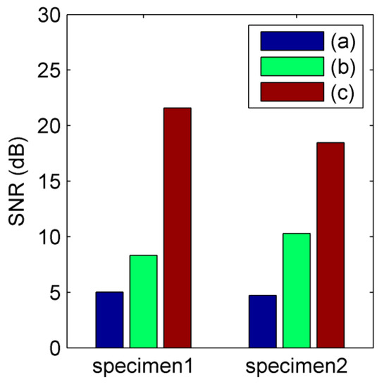
Figure 13.
The comparison of signal-to-noise ratio (SNR) for different specimens: (a) Conventional TFM; (b) TFM with hybrid full matrix; (c) SCF with the hybrid full matrix.
6. Future Work
The SCF algorithm is considered as a representative of the instantaneous phase and the sign bit of digitized received echo can be simply implemented by circuits and electronic components. It can quickly detect defects in rails and the operation is quite straightforward. However, considering that the retrieval of Green’s function is implemented by the cross-correlation of noise, the time of acquiring a hybrid full matrix will always be later than that of acquiring conventional full matrix. The calculation of Green’s function also takes some time. What’s more, the application of this method to other materials, such as aluminum, carbon fiber reinforced polymer, and so on, needs further verification. The extreme limitation of distance for the inspection system should be paid attention to. The work will be full of challenges and the detailed solution will be introduced in future work.
7. Conclusions
In this article, the near-surface defects in the rails are investigated and results show that optimal performance is achieved by SCF with a 32-element array. The following two conclusions can be made based on the investigation. The theory and data analysis indicate that the cross-correlation function can be exploited to reconstruct direct arrivals between any two elements. Thus, with a long time window over a large number of averages, the near-surface defect recognition is achieved by computing the cross-correlation of noise signals. What is more, in order to improve image quality, SCF is applied to weight the Green’s function. Its performance is quantitatively analyzed and compared with TFM. The results show that SCF images have better spatial resolution and SNR than TFM image. The use of SCF for near-surface imaging can potentially provide a reliable alternative to conventional implementations of defect detection.
Author Contributions
Conceptualization, H.Z.; data curation, W.Z.; formal analysis, H.Z.; funding acquisition, H.Z. and W.Z.; investigation, M.S.; methodology, M.S.; project administration, H.Z.; resources, G.F.; software, M.S.; supervision, G.F.; validation, Q.Z.; visualization, Hui Zhang; writing—original draft, M.S.; writing—review and editing, Q.Z.
Funding
This research was funded by the National Natural Science Foundation of China (Grant Nos. 11874255 and 11674214) and the Key Technology R&D Project of Shanghai Committee of Science and Technology (Grant No. 16030501400).
Acknowledgments
The authors wish to acknowledge the contributions of associates and colleagues at Shanghai University.
Conflicts of Interest
The authors declare no conflict of interest.
References
- Ahmad, R.; Kundu, T.; Placko, D. Modeling of phased array transducers. J. Acoust. Soc. Am. 2005, 117, 1762–1776. [Google Scholar] [CrossRef] [PubMed]
- Potter, J.N.; Wilcox, P.D.; Croxford, A.J. Diffuse field full matrix capture for near surface ultrasonic imaging. Ultrasonics 2018, 82, 44–48. [Google Scholar] [CrossRef] [PubMed]
- Rickett, J.; Claerbout, J. Acoustic daylight imaging via spectral factorization: Helioseismology and reservoir monitoring. Leading Edge 1999, 18, 957–960. [Google Scholar] [CrossRef]
- Lobkis, O.I.; Weaver, R.L. On the emergence of the Green’s function in the correlations of a diffuse field. J. Acoust. Soc. Am. 2001, 110, 3011–3017. [Google Scholar] [CrossRef]
- Davy, M.; Fink, M.; De Rosny, J. Green’s Function Retrieval and Passive Imaging from Correlations of Wideband Thermal Radiations. Phys. Rev. Lett. 2013, 110, 203901. [Google Scholar] [CrossRef]
- Stehly, L.; Campillo, M.; Froment, B.; Weaver, R.L. Reconstructing Green’s function by correlation of the coda of the correlation (C3) of ambient seismic noise. J. Geophys. Res. 2008, 113, B11306. [Google Scholar] [CrossRef]
- Froment, B.; Campillo, M.; Roux, P. Reconstructing the Green’s function through iteration of correlations. C.R. Geosci. 2011, 343, 623–632. [Google Scholar] [CrossRef]
- Sabra, K.G.; Roux, P.; Thode, A.M.; D’Spain, G.L.; Hodgkiss, W.S.; Kuperman, W.A. Using ocean ambient noise for array self-localization and self-synchronization. IEEE J. Ocean. Eng. 2005, 30, 338–347. [Google Scholar] [CrossRef]
- Farrar, C.R.; Iii, G.H.J. System identification from ambient vibration measurements on a bridge. J. Sound. Vib. 1997, 205, 1–18. [Google Scholar] [CrossRef]
- Sabra, K.G.; Conti, S.; Roux, P.; Kuperman, W.A. Passive in vivo elastography from skeletal muscle noise. Appl. Phys. Lett. 2007, 90, 194101. [Google Scholar] [CrossRef]
- Sabra, K.G.; Winkel, E.S.; Bourgoyne, D.A.; Elbing, B.R.; Ceccio, S.L.; Perlin, M.; Dowling, D.R. Using cross correlations of turbulent flow-induced ambient vibrations to estimate the structural impulse response. Application to structural health monitoring. J. Acoust. Soc. Am. 2007, 121, 1987–1995. [Google Scholar] [CrossRef] [PubMed]
- Snieder, R. Extracting the Green’s function from the correlation of coda waves: A derivation based on stationary phase. Phys. Rev. E 2004, 69, 046610. [Google Scholar] [CrossRef] [PubMed]
- Snieder, R. Retrieving the Green’s function of the diffusion equation from the response to a random forcing. Phys. Rev. E 2006, 74, 046620. [Google Scholar] [CrossRef] [PubMed]
- Moulin, E.; Abou Leyla, N.; Assaad, J.; Grondel, S. Applicability of acoustic noise correlation for structural health monitoring in nondiffuse field conditions. Appl. Phys. Lett. 2009, 95, 094104. [Google Scholar] [CrossRef]
- Colombi, A.; Boschi, L.; Roux, P.; Campillo, M. Green’s function retrieval through cross-correlations in a two-dimensional complex reverberating medium. J. Acoust. Soc. Am. 2014, 135, 1034–1043. [Google Scholar] [CrossRef] [PubMed]
- Chehami, L.; De Rosny, J.; Prada, C.; Moulin, E.; Assaad, J. Experimental study of passive defect localization in plates using ambient noise. IEEE Trans. Ultrason. Ferr. 2015, 62, 1544–1553. [Google Scholar] [CrossRef]
- Holmes, C.; Drinkwater, B.W.; Wilcox, P.D. Post-processing of the full matrix of ultrasonic transmit–receive array data for non-destructive evaluation. NDT e Int. 2005, 38, 701–711. [Google Scholar] [CrossRef]
- Camacho, J.; Parrilla, M.; Fritsch, C. Phase coherence imaging. IEEE Trans. Ultrason. Ferr. 2009, 56, 958–974. [Google Scholar] [CrossRef]
- Fan, G.; Zhang, H.; Zhu, W.; Zhang, H.; Chai, X. Numerical and experimental research on identifying a delamination in Ballastless slab track. Materials 2019, 12, 1788. [Google Scholar] [CrossRef]
- Derode, A.; Larose, E.; Tanter, M.; De Rosny, J.; Tourin, A.; Campillo, M.; Fink, M. Recovering the Green’s function from field-field correlations in an open scattering medium (L). J. Acoust. Soc. Am. 2003, 113, 2973–2976. [Google Scholar] [CrossRef]
- Weaver, R.L.; Lobkis, O.I. Diffuse fields in open systems and the emergence of the Green’s function (L). J. Acoust. Soc. Am. 2004, 116, 2731–2734. [Google Scholar] [CrossRef]
- Weaver, R.L.; Lobkis, O.I. Ultrasonics without a source: Thermal fluctuation correlations at MHz frequencies. Phys. Rev. Lett. 2001, 87, 134301. [Google Scholar] [CrossRef] [PubMed]
- Beke, D.L.; Daroczi, L.; Toth, L.Z.; Bolgar, M.K.; Samy, N.M.; Hudak, A. Acoustic emissions during structural changes in shape memory alloys. Metals 2019, 9, 58. [Google Scholar] [CrossRef]
- Chehami, L.; Moulin, E.; De Rosny, J.; Prada, C.; Matar, O.B.; Benmeddour, F.; Assaad, J. Detection and localization of a defect in a reverberant plate using acoustic field correlation. J. Appl. Phys. 2014, 115, 104901. [Google Scholar] [CrossRef]
- Hunter, A.J.; Drinkwater, B.W.; Wilcox, P.D. The wavenumber algorithm for full-matrix imaging using an ultrasonic array. IEEE Trans. Ultrason. Ferr. 2008, 55, 2450–2462. [Google Scholar] [CrossRef] [PubMed]


© 2019 by the authors. Licensee MDPI, Basel, Switzerland. This article is an open access article distributed under the terms and conditions of the Creative Commons Attribution (CC BY) license (http://creativecommons.org/licenses/by/4.0/).