Multi-Proxy Approach for Identifying Heinrich Events in Sediment Cores from Hatton Bank (NE Atlantic Ocean)

 , and
, and
Abstract
:1. Introduction
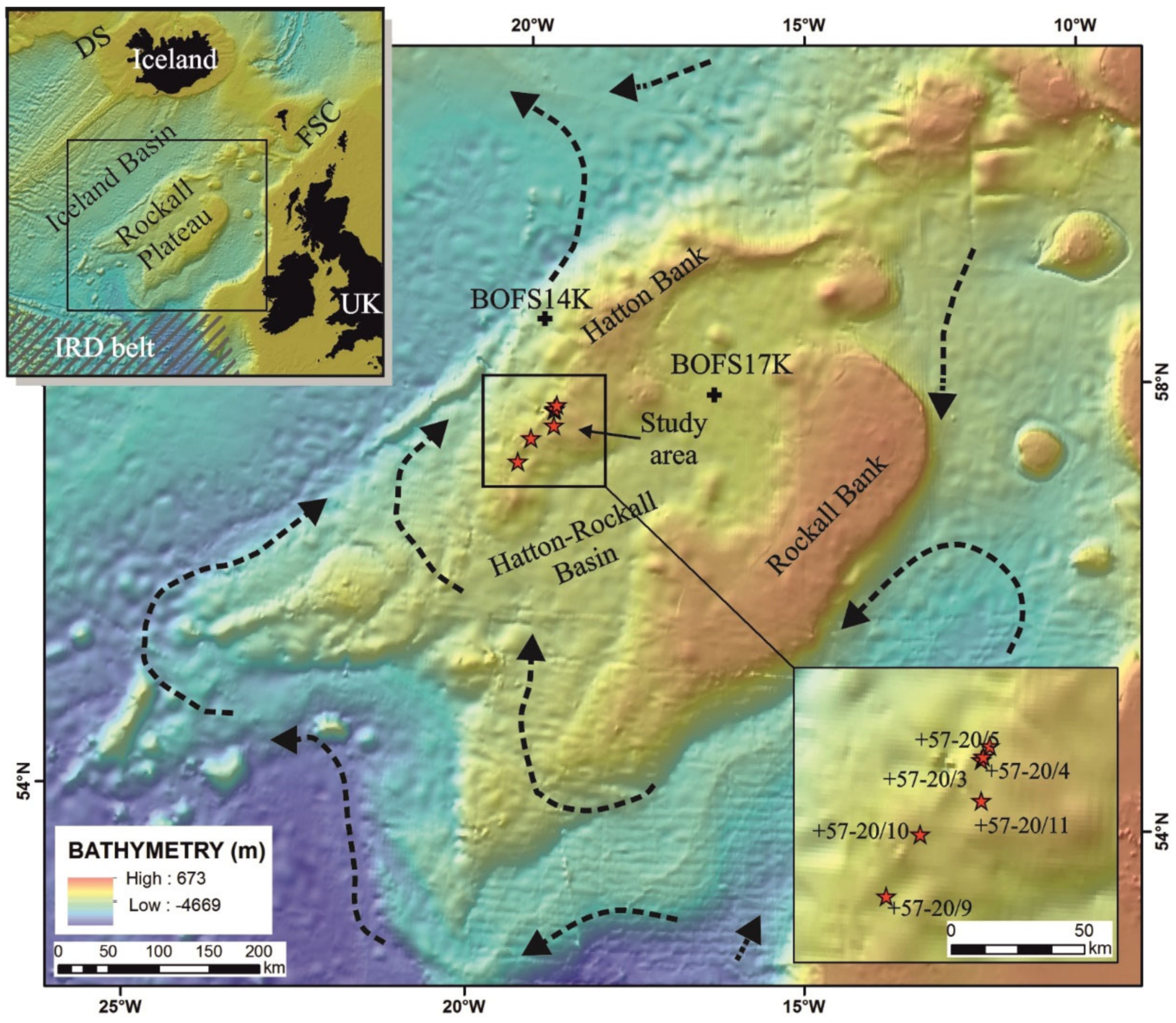
1.1. Setting
1.2. Oceanography
1.3. Heinrich Events
2. Materials and Methods
3. Results
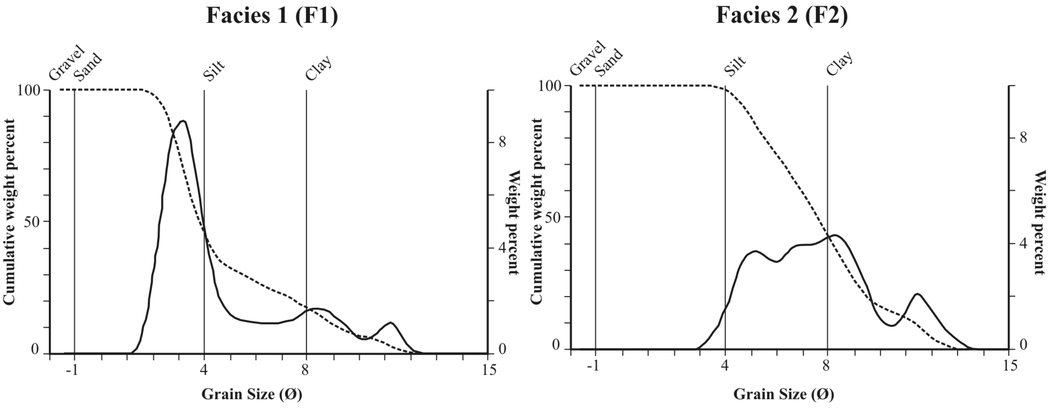
3.1. Sediment Facies
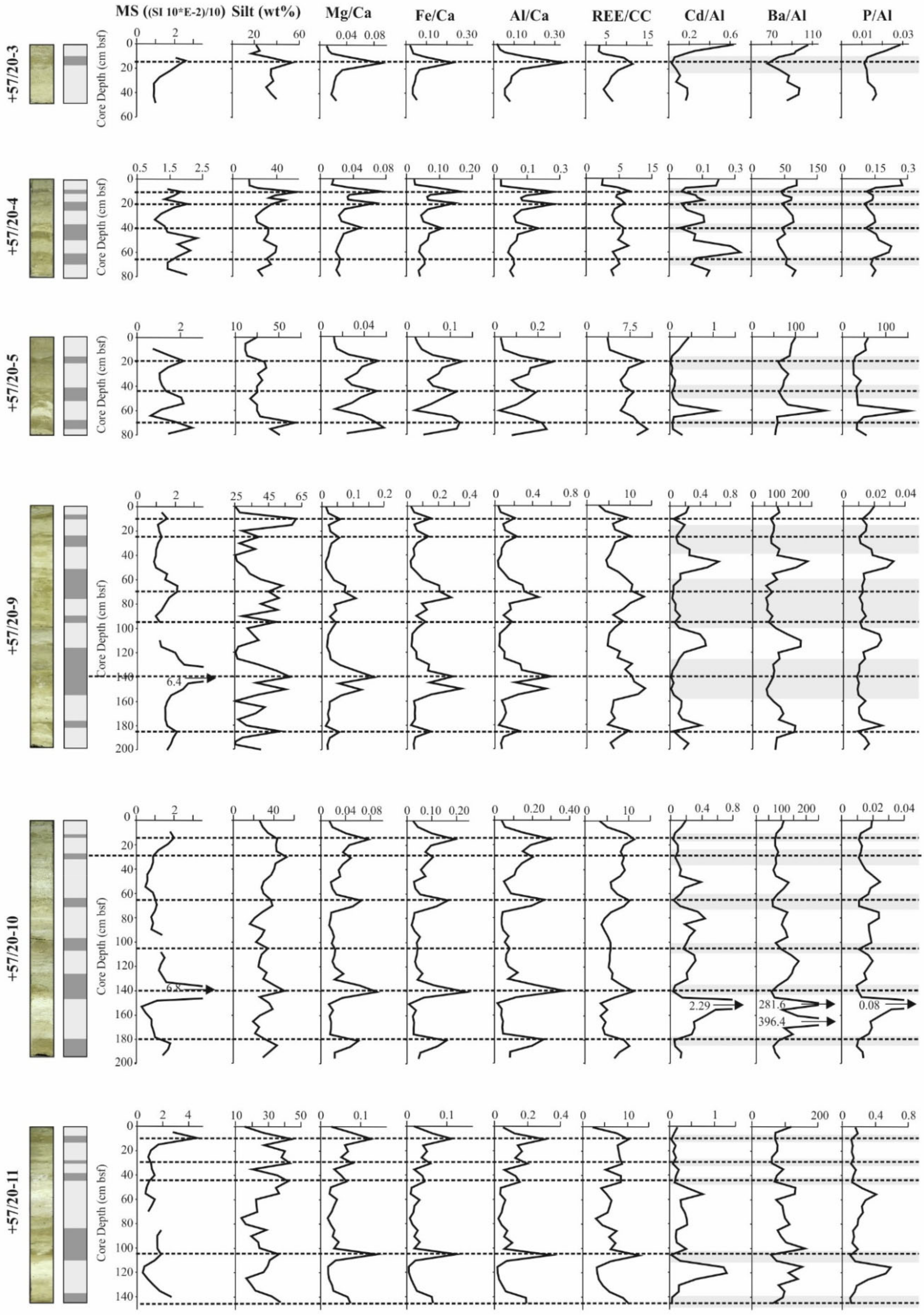
3.2. Proxies
3.3. Foraminifera Associations
4. Discussion
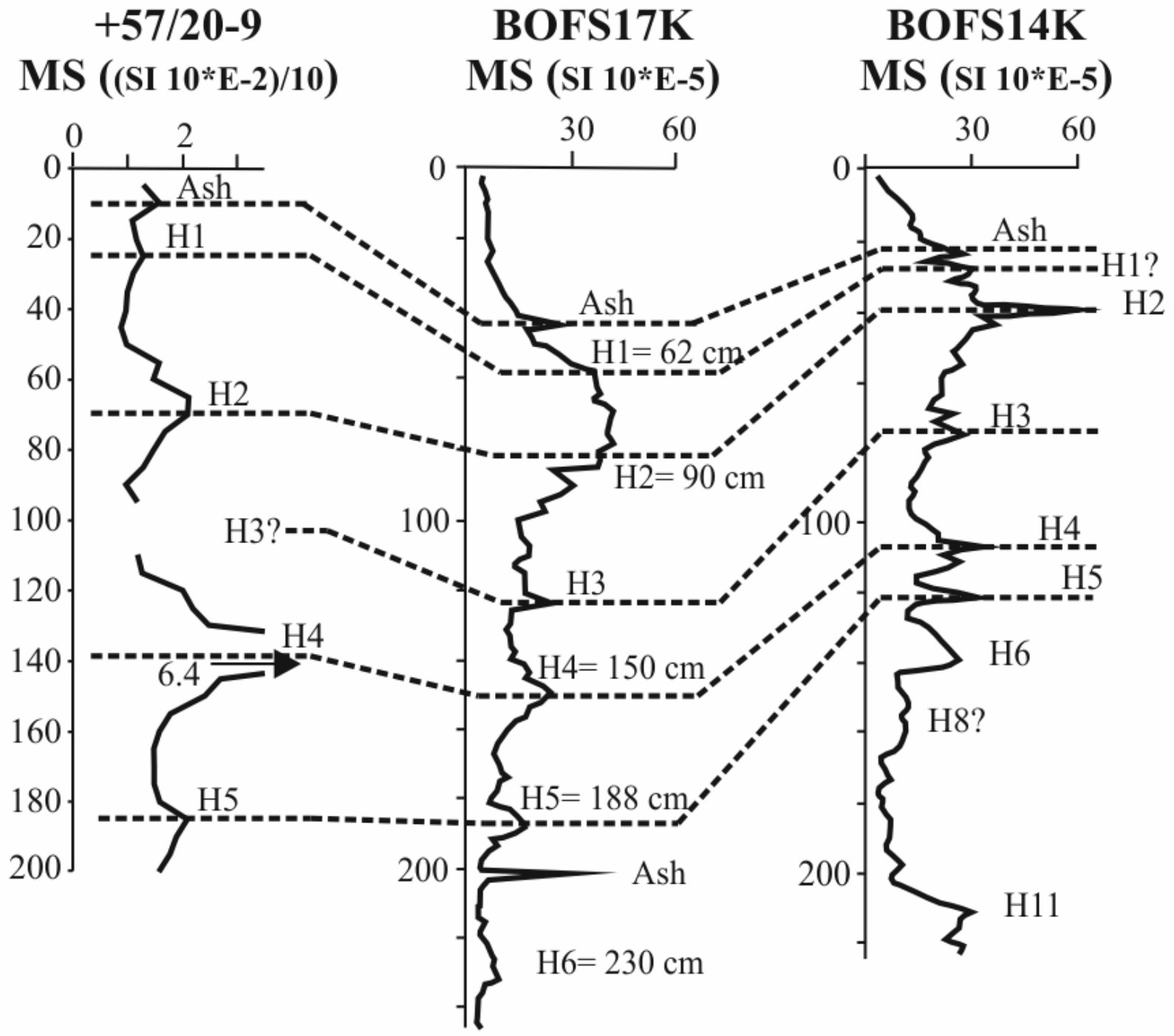
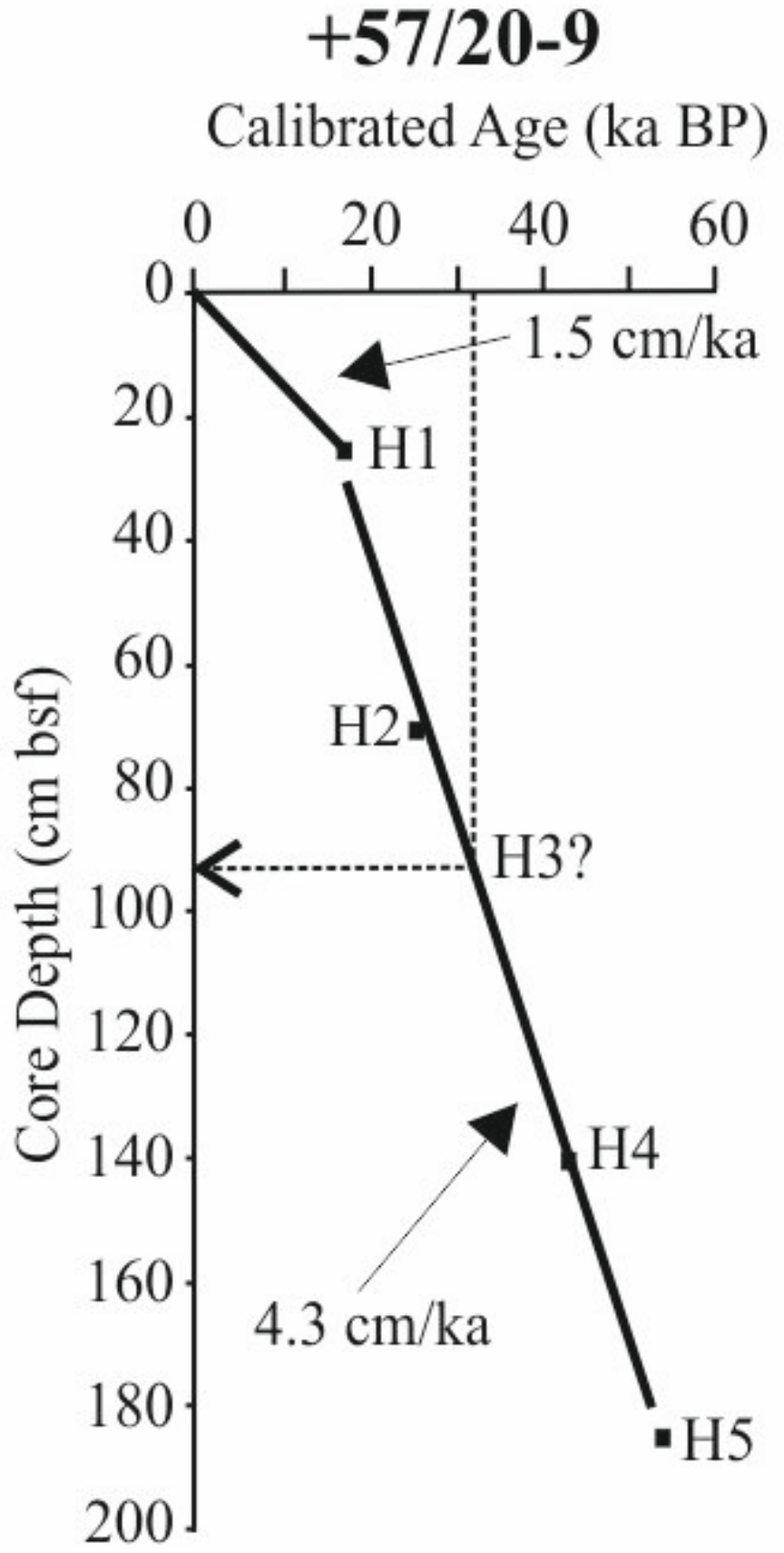
4.1. Age-Model Based on Identification of Heinrich Events
4.2. Chronostratigraphic Approximation and Reconstruction
5. Conclusions
Author Contributions
Funding
Acknowledgments
Conflicts of Interest
Appendix A

| Samples | Fe (%) | Cd (ppm) | Ca (%) | P (%) | Mg (%) | Ba (ppm) | Al (%) | Total_REE (CC) | Gravel (%) | Sand (%) | Silt (%) | Clay (%) |
|---|---|---|---|---|---|---|---|---|---|---|---|---|
| 57-20/3 0–1 | 0.69 | 0.57 | 33.39 | 0.020 | 0.35 | 78 | 0.74 | 3.13 | 0.00 | 73.64 | 22.06 | 4.31 |
| 57-20/3 5–6 | 0.84 | 0.35 | 28.35 | 0.022 | 0.41 | 103 | 1.10 | 2.97 | 0.00 | 71.16 | 25.19 | 3.65 |
| 57-20/3 7–8 | 0.98 | 0.34 | 26.55 | 0.025 | 0.49 | 138 | 1.50 | 4.09 | 0.00 | 79.59 | 17.88 | 2.54 |
| 57-20/3 10–11 | 2.13 | 0.30 | 21.85 | 0.040 | 0.93 | 257 | 3.35 | 8.59 | 7.00 | 45.58 | 32.97 | 14.46 |
| 57-20/3 15–16 | 3.07 | 0.25 | 13.71 | 0.050 | 1.24 | 316 | 4.80 | 10.56 | 0.00 | 29.99 | 53.53 | 16.48 |
| 57-20/3 20–21 | 1.47 | 0.30 | 21.04 | 0.034 | 0.72 | 229 | 2.95 | 7.41 | 0.00 | 40.71 | 35.25 | 24.04 |
| 57-20/3 25–26 | 1.17 | 0.34 | 23.58 | 0.027 | 0.60 | 200 | 2.30 | 5.87 | 0.00 | 47.55 | 34.88 | 17.57 |
| 57-20/3 30–31 | 1.12 | 0.22 | 24.12 | 0.026 | 0.56 | 183 | 2.14 | 5.27 | 0.00 | 50.53 | 37.36 | 12.12 |
| 57-20/3 35–36 | 0.88 | 0.36 | 26.43 | 0.024 | 0.54 | 155 | 1.60 | 4.12 | 0.00 | 56.95 | 30.58 | 12.47 |
| 57-20/3 40–41 | 0.88 | 0.40 | 27.14 | 0.027 | 0.50 | 162 | 1.69 | 5.00 | 0.00 | 46.07 | 35.16 | 18.77 |
| 57-20/3 45–46 | 1.31 | 0.48 | 24.88 | 0.032 | 0.62 | 192 | 2.26 | 6.26 | 0.00 | 36.35 | 40.61 | 23.04 |
| 57-20/4 0–1 | 0.72 | 0.23 | 30.99 | 0.021 | 0.51 | 94 | 0.92 | 3.43 | 0.00 | 82.44 | 14.61 | 2.96 |
| 57-20/4 5–6 | 0.79 | 0.22 | 30.86 | 0.022 | 0.44 | 95 | 0.93 | 3.21 | 0.00 | 81.73 | 15.38 | 2.90 |
| 57-20/4 7–8 | 1.74 | 0.21 | 22.85 | 0.034 | 0.80 | 214 | 2.56 | 6.67 | 0.00 | 70.94 | 22.64 | 6.42 |
| 57-20/4 10–11 | 2.59 | 0.27 | 15.90 | 0.042 | 1.20 | 281 | 4.27 | 9.68 | 0.00 | 25.19 | 58.25 | 16.57 |
| 57-20/4 13–14 | 1.51 | 0.39 | 20.68 | 0.036 | 0.75 | 215 | 2.94 | 6.81 | 0.00 | 38.91 | 38.61 | 22.48 |
| 57-20/4 15–16 | 1.34 | 0.37 | 21.68 | 0.032 | 0.73 | 235 | 2.58 | 6.59 | 0.00 | 39.87 | 33.76 | 26.38 |
| 57-20/4 17–18 | 1.45 | 0.48 | 22.16 | 0.033 | 0.76 | 253 | 2.78 | 7.61 | 0.00 | 19.22 | 48.01 | 32.77 |
| 57-20/4 20–21 | 2.13 | 0.25 | 14.74 | 0.035 | 0.98 | 272 | 3.94 | 8.55 | 0.00 | 44.16 | 35.84 | 20.01 |
| 57-20/4 25–26 | 1.39 | 0.23 | 21.32 | 0.027 | 0.65 | 212 | 2.58 | 6.27 | 0.00 | 61.40 | 27.68 | 10.92 |
| 57-20/4 30–31 | 1.02 | 0.34 | 22.44 | 0.025 | 0.52 | 185 | 1.98 | 5.57 | 0.00 | 64.94 | 21.31 | 13.75 |
| 57-20/4 35–36 | 1.14 | 0.38 | 22.11 | 0.028 | 0.58 | 202 | 2.14 | 6.21 | 0.00 | 59.75 | 22.37 | 17.88 |
| 57-20/4 40–41 | 1.98 | 0.20 | 18.18 | 0.034 | 0.90 | 249 | 3.62 | 8.20 | 0.00 | 48.04 | 32.46 | 19.50 |
| 57-20/4 45–46 | 1.65 | 0.33 | 24.14 | 0.034 | 0.70 | 193 | 2.53 | 8.15 | 0.00 | 55.80 | 31.82 | 12.38 |
| 57-20/4 50–51 | 1.71 | 0.33 | 26.47 | 0.038 | 0.68 | 153 | 2.64 | 7.03 | 1.19 | 54.65 | 28.50 | 15.66 |
| 57-20/4 55–56 | 1.25 | 0.67 | 29.49 | 0.042 | 0.65 | 134 | 2.16 | 9.56 | 3.60 | 23.21 | 40.31 | 32.89 |
| 57-20/4 60–61 | 1.07 | 0.62 | 28.47 | 0.032 | 0.56 | 125 | 1.74 | 5.84 | 0.00 | 35.26 | 39.46 | 25.28 |
| 57-20/4 65–66 | 1.50 | 0.32 | 27.70 | 0.029 | 0.66 | 188 | 2.38 | 6.72 | 1.03 | 53.95 | 31.12 | 13.91 |
| 57-20/4 70–71 | 1.57 | 0.29 | 28.46 | 0.029 | 0.67 | 200 | 2.55 | 7.35 | 0.00 | 53.32 | 35.57 | 11.12 |
| 57-20/4 75–76 | 0.97 | 0.38 | 26.91 | 0.025 | 0.53 | 187 | 1.87 | 5.40 | 2.20 | 61.78 | 23.14 | 12.88 |
| 57-20/4 80–81 | 1.01 | 0.39 | 24.31 | 0.025 | 0.59 | 194 | 2.11 | 5.94 | 6.06 | 58.01 | 27.63 | 8.30 |
| 57-20/5 0–1 | 0.58 | 0.48 | 32.70 | 0.018 | 0.39 | 85 | 0.80 | 3.30 | 0.00 | 62.28 | 30.73 | 7.00 |
| 57-20/5 5–6 | 0.72 | 0.39 | 31.54 | 0.018 | 0.41 | 86 | 0.89 | 3.37 | 0.00 | 76.23 | 19.27 | 4.51 |
| 57-20/5 10–11 | 1.08 | 0.33 | 32.76 | 0.024 | 0.48 | 108 | 1.15 | 3.61 | 0.00 | 77.99 | 19.16 | 2.86 |
| 57-20/5 15–16 | 1.40 | 0.24 | 23.76 | 0.028 | 0.61 | 219 | 2.41 | 5.97 | 0.00 | 73.43 | 21.17 | 5.41 |
| 57-20/5 20–21 | 2.30 | 0.24 | 18.27 | 0.039 | 0.95 | 253 | 4.00 | 8.81 | 0.00 | 44.28 | 36.90 | 18.82 |
| 57-20/5 25–26 | 1.57 | 0.28 | 19.59 | 0.027 | 0.74 | 199 | 2.71 | 6.45 | 0.00 | 42.38 | 38.57 | 19.05 |
| 57-20/5 30–31 | 1.35 | 0.19 | 18.87 | 0.025 | 0.63 | 218 | 2.47 | 6.02 | 0.00 | 55.77 | 31.24 | 12.99 |
| 57-20/5 35–36 | 1.15 | 0.31 | 24.43 | 0.026 | 0.57 | 126 | 1.62 | 5.31 | 0.00 | 56.50 | 34.96 | 8.54 |
| 57-20/5 40–41 | 1.35 | 0.36 | 22.58 | 0.026 | 0.64 | 159 | 2.15 | 5.71 | 0.00 | 57.40 | 30.11 | 12.49 |
| 57-20/5 45–46 | 2.15 | 0.31 | 19.17 | 0.037 | 0.99 | 198 | 3.01 | 7.17 | 0.00 | 54.26 | 30.26 | 15.49 |
| 57-20/5 50–51 | 1.60 | 0.36 | 19.71 | 0.033 | 0.73 | 181 | 2.46 | 6.23 | 0.00 | 59.95 | 23.75 | 16.31 |
| 57-20/5 55–56 | 1.26 | 0.59 | 23.20 | 0.028 | 0.66 | 173 | 1.99 | 5.88 | 0.00 | 42.75 | 30.14 | 27.12 |
| 57-20/5 60–61 | 0.51 | 0.86 | 30.47 | 0.036 | 0.40 | 107 | 0.60 | 5.30 | 0.00 | 23.79 | 29.92 | 46.29 |
| 57-20/5 65–66 | 1.95 | 0.33 | 19.14 | 0.042 | 0.73 | 136 | 2.22 | 7.23 | 1.36 | 44.64 | 33.00 | 21.00 |
| 57-20/5 70–71 | 2.04 | 0.33 | 16.87 | 0.039 | 0.83 | 189 | 3.03 | 7.99 | 0.00 | 7.61 | 64.70 | 27.69 |
| 57-20/5 75–76 | 2.01 | 0.45 | 17.66 | 0.044 | 1.02 | 202 | 3.51 | 9.34 | 0.00 | 20.99 | 42.20 | 36.81 |
| 57-20/5 80–81 | 0.93 | 0.70 | 25.48 | 0.037 | 0.61 | 95 | 1.70 | 7.74 | 0.00 | 8.30 | 50.79 | 40.91 |
| 57-20/9 0–1 | 0.68 | 0.24 | 28.90 | 0.020 | 0.39 | 101 | 0.97 | 2.73 | 0.00 | 72.29 | 24.71 | 3.01 |
| 57-20/9 5–6 | 1.14 | 0.32 | 25.04 | 0.026 | 0.53 | 173 | 1.52 | 4.31 | 0.00 | 61.60 | 27.95 | 10.46 |
| 57-20/9 10–11 | 2.56 | 0.19 | 16.88 | 0.045 | 1.00 | 273 | 3.59 | 9.21 | 0.00 | 22.21 | 61.70 | 16.09 |
| 57-20/9 15–16 | 1.07 | 0.39 | 22.94 | 0.030 | 0.54 | 180 | 1.99 | 5.98 | 0.00 | 11.39 | 59.04 | 29.58 |
| 57-20/9 20–21 | 1.36 | 0.32 | 21.79 | 0.034 | 0.61 | 208 | 2.35 | 6.49 | 0.00 | 49.57 | 29.38 | 21.06 |
| 57-20/9 25–26 | 2.42 | 0.33 | 17.89 | 0.043 | 0.99 | 328 | 4.20 | 9.91 | 0.00 | 34.69 | 39.25 | 26.07 |
| 57-20/9 30–31 | 1.36 | 0.26 | 21.49 | 0.027 | 0.67 | 191 | 2.36 | 6.58 | 0.00 | 55.10 | 27.86 | 17.04 |
| 57-20/9 35–36 | 0.95 | 0.44 | 23.68 | 0.031 | 0.57 | 194 | 1.69 | 6.01 | 0.00 | 33.88 | 37.04 | 29.08 |
| 57-20/9 40–41 | 1.19 | 0.42 | 25.66 | 0.031 | 0.55 | 171 | 1.63 | 5.38 | 0.00 | 51.63 | 24.42 | 23.95 |
| 57-20/9 45–46 | 0.68 | 0.59 | 30.04 | 0.030 | 0.40 | 212 | 0.92 | 4.44 | 0.00 | 55.08 | 26.32 | 18.60 |
| 57-20/9 50–51 | 0.76 | 0.52 | 28.67 | 0.030 | 0.41 | 194 | 1.06 | 4.94 | 0.00 | 50.74 | 31.11 | 18.15 |
| 57-20/9 55–56 | 1.76 | 0.35 | 27.07 | 0.034 | 0.73 | 222 | 2.57 | 7.29 | 0.00 | 56.13 | 33.83 | 10.04 |
| 57-20/9 60–61 | 1.90 | 0.39 | 19.00 | 0.039 | 0.76 | 292 | 2.83 | 9.03 | 0.00 | 40.78 | 40.36 | 18.87 |
| 57-20/9 65–66 | 3.06 | 0.20 | 14.91 | 0.053 | 1.14 | 256 | 4.36 | 10.45 | 11.03 | 16.04 | 53.25 | 19.68 |
| 57-20/9 70–71 | 2.91 | 0.21 | 14.11 | 0.056 | 1.05 | 362 | 4.37 | 10.19 | 0.00 | 25.83 | 45.05 | 29.12 |
| 57-20/9 75–76 | 3.28 | 0.16 | 11.66 | 0.057 | 1.26 | 305 | 5.42 | 13.19 | 0.00 | 22.73 | 51.11 | 26.16 |
| 57-20/9 80–81 | 2.18 | 0.25 | 23.16 | 0.044 | 0.93 | 237 | 3.57 | 10.03 | 0.00 | 32.66 | 40.56 | 26.78 |
| 57-20/9 85–86 | 2.44 | 0.22 | 19.41 | 0.040 | 0.90 | 204 | 3.27 | 8.44 | 3.33 | 26.33 | 50.32 | 20.02 |
| 57-20/9 90–91 | 1.39 | 0.28 | 23.64 | 0.031 | 0.65 | 178 | 2.12 | 6.12 | 0.81 | 55.65 | 29.31 | 14.23 |
| 57-20/9 95–96 | 2.14 | 0.21 | 18.47 | 0.036 | 0.85 | 233 | 3.31 | 8.34 | 0.00 | 35.39 | 49.54 | 15.07 |
| 57-20/9 100–101 | 1.37 | 0.31 | 20.40 | 0.030 | 0.66 | 243 | 2.46 | 6.50 | 0.00 | 58.57 | 32.47 | 8.96 |
| 57-20/9 105–106 | 0.90 | 0.52 | 25.74 | 0.031 | 0.54 | 193 | 1.32 | 5.27 | 0.00 | 45.20 | 35.76 | 19.03 |
| 57-20/9 110–111 | 0.82 | 0.63 | 26.82 | 0.034 | 0.53 | 280 | 1.38 | 4.96 | 0.00 | 37.74 | 39.37 | 22.89 |
| 57-20/9 115–116 | 0.78 | 0.58 | 27.20 | 0.027 | 0.51 | 245 | 1.22 | 4.81 | 0.00 | 62.90 | 27.08 | 10.02 |
| 57-20/9 120–121 | 1.54 | 0.49 | 25.94 | 0.034 | 0.68 | 285 | 2.62 | 7.63 | 0.00 | 62.64 | 25.41 | 11.96 |
| 57-20/9 125–126 | 1.59 | 0.32 | 26.27 | 0.036 | 0.74 | 293 | 2.55 | 7.03 | 0.00 | 63.01 | 26.60 | 10.40 |
| 57-20/9 130–131 | 2.42 | 0.38 | 17.21 | 0.049 | 1.00 | 396 | 4.57 | 10.43 | 0.00 | 34.13 | 38.69 | 27.19 |
| 57-20/9 133–134 | 1.72 | 0.34 | 18.29 | 0.041 | 0.96 | 385 | 3.87 | 8.83 | 5.86 | 20.22 | 49.67 | 24.25 |
| 57-20/9 135–136 | 2.04 | 0.15 | 15.33 | 0.045 | 1.71 | 402 | 4.38 | 8.86 | 0.00 | 11.65 | 50.04 | 38.32 |
| 57-20/9 140–141 | 2.63 | 0.11 | 9.01 | 0.048 | 1.52 | 479 | 5.42 | 10.39 | 0.00 | 3.55 | 58.01 | 38.45 |
| 57-20/9 145–146 | 2.52 | 0.18 | 17.58 | 0.039 | 0.96 | 289 | 3.83 | 10.87 | 7.26 | 45.74 | 37.74 | 9.27 |
| 57-20/9 150–151 | 3.71 | 0.11 | 10.82 | 0.054 | 1.38 | 345 | 5.84 | 13.45 | 0.00 | 20.10 | 55.14 | 24.76 |
| 57-20/9 155–156 | 2.68 | 0.22 | 17.46 | 0.044 | 1.09 | 283 | 4.34 | 11.89 | 0.00 | 36.64 | 38.76 | 24.60 |
| 57-20/9 160–161 | 1.26 | 0.31 | 27.98 | 0.029 | 0.70 | 181 | 2.02 | 6.22 | 0.00 | 60.84 | 23.88 | 15.28 |
| 57-20/9 165–166 | 1.27 | 0.38 | 25.48 | 0.027 | 0.62 | 307 | 2.60 | 6.05 | 10.77 | 21.61 | 42.73 | 24.90 |
| 57-20/9 170–171 | 1.05 | 0.29 | 22.27 | 0.027 | 0.46 | 335 | 2.59 | 5.59 | 0.00 | 41.97 | 37.30 | 20.74 |
| 57-20/9 175–176 | 1.30 | 0.38 | 25.57 | 0.029 | 0.59 | 261 | 2.35 | 6.47 | 0.00 | 53.88 | 26.79 | 19.33 |
| 57-20/9 180–181 | 0.79 | 0.50 | 29.33 | 0.031 | 0.39 | 222 | 1.23 | 4.80 | 0.00 | 42.86 | 31.98 | 25.16 |
| 57-20/9 185–186 | 2.53 | 0.22 | 16.76 | 0.041 | 0.94 | 757 | 4.30 | 9.68 | 0.00 | 35.15 | 51.86 | 12.99 |
| 57-20/9 190–191 | 1.47 | 0.35 | 27.05 | 0.035 | 0.68 | 255 | 2.48 | 7.48 | 0.00 | 50.63 | 29.52 | 19.85 |
| 57-20/9 195–196 | 1.22 | 0.46 | 29.32 | 0.031 | 0.54 | 183 | 1.87 | 5.49 | 2.13 | 43.37 | 23.03 | 31.47 |
| 57-20/9 200–201 | 1.29 | 0.38 | 28.26 | 0.029 | 0.56 | 203 | 2.12 | 6.29 | 0.00 | 46.47 | 40.71 | 12.82 |
| 57-20/10 0–1 | 0.85 | 0.24 | 31.27 | 0.023 | 0.45 | 130 | 1.18 | 3.51 | 0.00 | 68.56 | 25.96 | 5.48 |
| 57-20/10 5–6 | 1.28 | 0.23 | 28.77 | 0.030 | 0.53 | 161 | 1.60 | 5.07 | 0.00 | 62.59 | 29.18 | 8.23 |
| 57-20/10 10–11 | 2.19 | 0.21 | 21.70 | 0.039 | 0.88 | 265 | 3.26 | 9.45 | 7.14 | 50.19 | 34.36 | 8.30 |
| 57-20/10 15–16 | 2.98 | 0.16 | 15.37 | 0.050 | 1.17 | 349 | 4.60 | 11.32 | 0.00 | 43.14 | 43.79 | 13.07 |
| 57-20/10 20–21 | 1.94 | 0.36 | 19.60 | 0.048 | 0.89 | 288 | 3.75 | 8.89 | 0.00 | 29.85 | 42.29 | 27.86 |
| 57-20/10 25–26 | 1.61 | 0.31 | 20.97 | 0.038 | 0.75 | 274 | 3.11 | 8.15 | 0.00 | 26.94 | 43.07 | 29.99 |
| 57-20/10 30–31 | 1.95 | 0.24 | 18.51 | 0.040 | 0.89 | 290 | 3.71 | 8.93 | 0.00 | 20.16 | 52.63 | 27.21 |
| 57-20/10 35–36 | 1.67 | 0.33 | 22.08 | 0.041 | 0.78 | 254 | 3.18 | 8.48 | 0.00 | 36.18 | 41.78 | 22.04 |
| 57-20/10 40–41 | 1.50 | 0.39 | 25.39 | 0.044 | 0.74 | 200 | 2.87 | 9.10 | 0.75 | 26.85 | 40.43 | 31.98 |
| 57-20/10 45–46 | 1.75 | 0.30 | 23.58 | 0.050 | 0.73 | 199 | 2.49 | 8.08 | 0.00 | 37.12 | 37.78 | 25.11 |
| 57-20/10 50–51 | 0.82 | 0.59 | 30.01 | 0.037 | 0.51 | 194 | 1.50 | 5.88 | 0.00 | 46.17 | 30.41 | 23.42 |
| 57-20/10 55–56 | 0.94 | 0.34 | 27.19 | 0.033 | 0.50 | 200 | 1.81 | 6.08 | 0.67 | 48.47 | 28.30 | 22.56 |
| 57-20/10 60–61 | 1.43 | 0.31 | 26.47 | 0.039 | 0.66 | 197 | 2.30 | 7.35 | 0.00 | 45.73 | 30.07 | 24.20 |
| 57-20/10 65–66 | 2.73 | 0.19 | 16.47 | 0.048 | 1.07 | 283 | 4.34 | 10.13 | 0.00 | 43.21 | 37.00 | 19.79 |
| 57-20/10 70–71 | 2.22 | 0.46 | 18.72 | 0.040 | 0.96 | 243 | 3.65 | 8.84 | 0.00 | 36.62 | 38.91 | 24.47 |
| 57-20/10 75–76 | 1.02 | 0.48 | 31.68 | 0.032 | 0.54 | 169 | 1.34 | 6.03 | 0.00 | 40.95 | 28.72 | 30.33 |
| 57-20/10 80–81 | 0.81 | 0.53 | 31.14 | 0.028 | 0.49 | 131 | 1.18 | 4.49 | 0.00 | 53.92 | 21.56 | 24.53 |
| 57-20/10 85–86 | 0.69 | 0.23 | 33.51 | 0.021 | 0.44 | 125 | 1.22 | 3.77 | 0.00 | 77.59 | 16.61 | 5.81 |
| 57-20/10 87–88 | 0.71 | 0.35 | 29.10 | 0.022 | 0.45 | 120 | 1.11 | 4.14 | 0.00 | 78.41 | 17.48 | 4.11 |
| 57-20/10 90–91 | 0.76 | 0.36 | 24.91 | 0.020 | 0.45 | 134 | 1.14 | 4.33 | 0.00 | 57.25 | 31.12 | 11.63 |
| 57-20/10 95–96 | 1.35 | 0.48 | 25.96 | 0.035 | 0.55 | 242 | 1.92 | 5.13 | 0.00 | 57.95 | 27.76 | 14.29 |
| 57-20/10 100–101 | 1.24 | 0.35 | 30.86 | 0.031 | 0.55 | 128 | 1.64 | 5.72 | 0.00 | 59.32 | 22.70 | 17.99 |
| 57-20/10 105–106 | 1.05 | 0.31 | 23.45 | 0.020 | 0.54 | 187 | 1.83 | 5.84 | 0.00 | 55.26 | 34.41 | 10.33 |
| 57-20/10 110–111 | 1.10 | 0.52 | 27.47 | 0.029 | 0.60 | 239 | 1.70 | 5.62 | 0.00 | 58.90 | 28.31 | 12.79 |
| 57-20/10 115–116 | 0.98 | 0.56 | 29.65 | 0.034 | 0.54 | 295 | 1.72 | 5.55 | 0.00 | 54.63 | 26.43 | 18.95 |
| 57-20/10 120–121 | 1.14 | 0.54 | 28.09 | 0.035 | 0.64 | 309 | 2.05 | 5.43 | 0.00 | 55.49 | 25.15 | 19.37 |
| 57-20/10 125–126 | 1.37 | 0.56 | 21.79 | 0.038 | 0.79 | 381 | 2.68 | 6.33 | 0.00 | 48.74 | 32.82 | 18.44 |
| 57-20/10 130–131 | 1.21 | 0.45 | 28.18 | 0.032 | 0.63 | 258 | 2.04 | 6.12 | 0.00 | 54.33 | 30.03 | 15.64 |
| 57-20/10 135–136 | 2.00 | 0.24 | 17.99 | 0.037 | 1.12 | 336 | 3.86 | 8.50 | 0.00 | 38.09 | 39.79 | 22.12 |
| 57-20/10 137–138 | 1.83 | 0.25 | 21.07 | 0.035 | 0.80 | 262 | 2.95 | 8.28 | 0.85 | 39.39 | 44.05 | 15.71 |
| 57-20/10 140–141 | 3.24 | 0.18 | 13.62 | 0.052 | 1.23 | 308 | 5.01 | 11.04 | 0.00 | 30.10 | 50.38 | 19.52 |
| 57-20/10 145–146 | 1.60 | 0.44 | 24.06 | 0.036 | 0.82 | 208 | 2.79 | 6.61 | 0.00 | 44.20 | 26.39 | 29.41 |
| 57-20/10 150–151 | 0.31 | 1.12 | 37.05 | 0.040 | 0.47 | 138 | 0.49 | 3.55 | 0.00 | 5.05 | 35.37 | 59.59 |
| 57-20/10 152–153 | 0.21 | 1.13 | 37.88 | 0.040 | 0.44 | 80 | 0.40 | 3.26 | 0.00 | 7.14 | 29.88 | 62.99 |
| 57-20/10 155–156 | 1.28 | 0.73 | 34.56 | 0.040 | 0.68 | 134 | 1.26 | 5.02 | 0.00 | 29.90 | 39.05 | 31.05 |
| 57-20/10 160–161 | 0.80 | 0.51 | 33.18 | 0.028 | 0.49 | 189 | 1.14 | 3.53 | 0.00 | 47.39 | 26.25 | 26.37 |
| 57-20/10 165–166 | 0.91 | 0.43 | 31.61 | 0.026 | 0.51 | 555 | 1.40 | 4.65 | 0.00 | 60.27 | 19.89 | 19.84 |
| 57-20/10 170–171 | 0.87 | 0.41 | 31.79 | 0.025 | 0.51 | 146 | 1.30 | 4.05 | 0.00 | 61.80 | 25.89 | 12.31 |
| 57-20/10 175–176 | 0.94 | 0.40 | 33.20 | 0.025 | 0.50 | 210 | 1.44 | 4.57 | 0.00 | 58.75 | 21.80 | 19.46 |
| 57-20/10 180–181 | 2.67 | 0.23 | 16.75 | 0.046 | 1.01 | 395 | 4.34 | 8.90 | 1.56 | 54.76 | 31.94 | 11.74 |
| 57-20/10 185–186 | 2.45 | 0.24 | 19.87 | 0.038 | 0.94 | 277 | 3.95 | 10.21 | 0.00 | 36.95 | 43.21 | 19.85 |
| 57-20/10 190–191 | 1.44 | 0.31 | 26.63 | 0.029 | 0.60 | 167 | 2.17 | 7.88 | 0.00 | 49.36 | 36.18 | 14.46 |
| 57-20/10 195–196 | 1.26 | 0.27 | 25.92 | 0.029 | 0.58 | 196 | 2.08 | 6.66 | 0.00 | 61.65 | 29.11 | 9.25 |
| 57-20/11 0–1 | 0.61 | 0.17 | 20.49 | 0.016 | 0.34 | 123 | 1.00 | 2.34 | 0.00 | 81.84 | 15.52 | 2.64 |
| 57-20/11 5–6 | 2.57 | 0.28 | 22.03 | 0.049 | 1.03 | 198 | 2.63 | 7.90 | 0.00 | 61.43 | 27.09 | 11.47 |
| 57-20/11 10–11 | 3.05 | 0.17 | 15.01 | 0.048 | 1.14 | 340 | 4.55 | 10.48 | 0.89 | 41.84 | 44.21 | 13.06 |
| 57-20/11 15–16 | 1.57 | 0.39 | 21.07 | 0.038 | 0.77 | 244 | 2.97 | 7.97 | 23.08 | 26.48 | 27.58 | 22.86 |
| 57-20/11 20–21 | 1.83 | 0.30 | 20.28 | 0.040 | 0.84 | 271 | 3.36 | 8.30 | 0.00 | 35.51 | 40.44 | 24.06 |
| 57-20/11 25–26 | 1.76 | 0.43 | 25.33 | 0.043 | 0.79 | 204 | 3.11 | 8.49 | 0.90 | 29.90 | 37.93 | 31.27 |
| 57-20/11 30–31 | 2.11 | 0.27 | 19.54 | 0.041 | 0.93 | 250 | 3.85 | 8.98 | 0.00 | 32.34 | 43.38 | 24.28 |
| 57-20/11 35–36 | 0.91 | 0.32 | 26.95 | 0.026 | 0.55 | 156 | 1.58 | 5.30 | 0.00 | 63.27 | 20.62 | 16.12 |
| 57-20/11 40–41 | 1.66 | 0.43 | 23.76 | 0.040 | 0.75 | 236 | 2.96 | 8.81 | 0.00 | 34.58 | 35.49 | 29.94 |
| 57-20/11 45–46 | 1.77 | 0.38 | 22.05 | 0.040 | 0.86 | 242 | 3.35 | 8.79 | 0.00 | 20.31 | 42.09 | 37.60 |
| 57-20/11 50–51 | 0.68 | 0.41 | 30.32 | 0.026 | 0.48 | 143 | 1.06 | 4.29 | 0.00 | 36.09 | 34.77 | 29.14 |
| 57-20/11 55–56 | 0.60 | 0.79 | 32.86 | 0.043 | 0.44 | 140 | 1.05 | 5.57 | 0.00 | 2.93 | 36.75 | 60.33 |
| 57-20/11 60–61 | 1.76 | 0.48 | 30.10 | 0.054 | 0.75 | 150 | 1.93 | 6.62 | 10.00 | 40.13 | 22.62 | 27.25 |
| 57-20/11 65–66 | 1.08 | 0.41 | 31.67 | 0.037 | 0.63 | 150 | 1.56 | 6.24 | 0.00 | 60.81 | 22.71 | 16.48 |
| 57-20/11 70–71 | 0.95 | 0.48 | 32.62 | 0.035 | 0.54 | 137 | 1.38 | 5.72 | 0.00 | 49.96 | 23.33 | 26.72 |
| 57-20/11 75–76 | 0.42 | 0.27 | 33.29 | 0.014 | 0.36 | 74 | 0.71 | 3.03 | 0.00 | 82.32 | 13.38 | 4.30 |
| 57-20/11 80–81 | 0.77 | 0.50 | 31.03 | 0.023 | 0.48 | 145 | 1.24 | 4.55 | 0.00 | 75.08 | 16.27 | 8.65 |
| 57-20/11 85–86 | 1.45 | 0.34 | 29.77 | 0.029 | 0.61 | 182 | 2.21 | 7.76 | 0.00 | 60.46 | 28.84 | 10.70 |
| 57-20/11 90–91 | 1.04 | 0.23 | 30.09 | 0.024 | 0.54 | 153 | 1.66 | 6.12 | 0.00 | 77.01 | 19.59 | 3.40 |
| 57-20/11 95–96 | 1.51 | 0.42 | 25.20 | 0.033 | 0.70 | 283 | 2.65 | 7.55 | 0.00 | 56.33 | 23.79 | 19.88 |
| 57-20/11 100–101 | 1.06 | 0.64 | 30.62 | 0.032 | 0.61 | 280 | 1.71 | 6.44 | 0.00 | 53.47 | 24.45 | 22.08 |
| 57-20/11 105–106 | 3.26 | 0.20 | 14.51 | 0.049 | 1.21 | 306 | 4.96 | 12.88 | 12.41 | 28.63 | 36.44 | 22.53 |
| 57-20/11 110–111 | 1.13 | 0.49 | 29.54 | 0.033 | 0.67 | 163 | 2.08 | 6.47 | 0.00 | 37.63 | 30.95 | 31.42 |
| 57-20/11 115–116 | 0.31 | 0.63 | 35.94 | 0.030 | 0.41 | 79 | 0.51 | 3.28 | 0.00 | 32.60 | 29.52 | 37.88 |
| 57-20/11 120–121 | 0.36 | 0.80 | 36.15 | 0.032 | 0.41 | 70 | 0.61 | 3.43 | 0.00 | 16.72 | 27.07 | 56.21 |
| 57-20/11 125–126 | 0.67 | 0.55 | 35.83 | 0.028 | 0.45 | 126 | 0.89 | 3.79 | 0.00 | 58.79 | 16.36 | 24.85 |
| 57-20/11 130–131 | 0.90 | 0.28 | 29.09 | 0.023 | 0.50 | 111 | 1.30 | 4.67 | 0.00 | 72.98 | 19.31 | 7.71 |
| 57-20/11 135–136 | 1.29 | 0.39 | 28.28 | 0.028 | 0.54 | 191 | 1.86 | 6.17 | 0.00 | 60.37 | 22.12 | 17.51 |
| 57-20/11 140–141 | 2.24 | 0.23 | 19.86 | 0.036 | 0.81 | 366 | 3.76 | 9.26 | 0.00 | 55.32 | 32.00 | 12.68 |
| 57-20/11 145–146 | 2.43 | 0.21 | 20.56 | 0.043 | 0.92 | 266 | 3.92 | 10.63 | 0.00 | 45.66 | 37.64 | 16.71 |
References
- MacLachlan, S.E.; Elliot, G.M.; Parson, L.M. Investigations of the bottom current sculpted margin of Hatton bank, NE Atlantic. Mar Geol. 2008, 253, 170–184. [Google Scholar] [CrossRef]
- Hitchen, K. The geology of the UK Hatton–Rockall margin. Mar. Pet. Geol. 2004, 21, 993–1012. [Google Scholar] [CrossRef]
- Stow, D.A.V.; Lovell, J.P.B. Contourites: Their recognition in modern and ancient sediments. Earth Sci. Rev. 1979, 14, 251–291. [Google Scholar] [CrossRef]
- Stow, D.; Holbrook, J.A. Hatton Drift contourites, Northeast Atlantic, Deep Sea Drilling Project LEG 81. In Initial Reports DSDP; Roberts, D.G., Schnitker, D., Eds.; ODP Proceedings Series; American Geoscience Instiute: Washington, DC, USA, 1983; Volume 81. [Google Scholar]
- Ruddiman, W.F. Sediment redistribution on the Reykjanes Ridge: Seismic evidence. Geol. Soc. Am. Bull. 1972, 82, 2039–2062. [Google Scholar] [CrossRef]
- McCave, I.N.; Tucholke, B.E. Deep–current controlled sedimentation in the Western North Atlantic. In The geology of North America, The Western North Atlantic Region, Decade of North American Geology; Vogt, P.R., Tucholke, B.E., Eds.; Geological Society of America: Boulder, CO, USA, 1986; Volume M, pp. 451–467. [Google Scholar]
- Faugères, J.C.; Mézerais, M.L.; Stow, D.A.V. Contourite drift types and their distribution in the North and South Atlantic Ocean Basins. Sed Geol. 1993, 82, 189–203. [Google Scholar] [CrossRef]
- Faugères, J.C.; Stow, D.A.V.; Imbert, P.; Viana, A.R. Seismic features diagnostic of contourite drifts. Mar Geol. 1999, 162, 1–38. [Google Scholar] [CrossRef]
- McCave, I.N.; Lonsdale, P.F.; Hollister, C.D.; Gardner, W.D. Sediment transport over the Hatton and Gardar contourite drifts. J. Sed. Petrol. 1980, 50, 1049–1062. [Google Scholar]
- Bianchi, G.G.; McCave, I.N. Hydrography and sedimentation under the deep western boundary current on Björn and Gardar Drifts, Iceland Basin. Mar Geol. 2000, 165, 137–169. [Google Scholar] [CrossRef]
- Huizhong, W.; McCave, I.N. Distinguishing climatic and current effects in mid–Pleistocene sediments of Hatton and Gardar Drifts, NE Atlantic. J. Geol. Soc. Lond. 1990, 147, 373–383. [Google Scholar] [CrossRef]
- Weaver, P.P.E.; Wynn, R.B.; Kenyon, N.H.; Evans, J. Continental margin sedimentation, with special reference to the north–east Atlantic margin. Sedimentology 2000, 47, 239–256. [Google Scholar] [CrossRef]
- Stow, D.A.V.; Holbrook, J.A. Hatton Drift contourites, northeast Atlantic, deep sea drilling project LEG 81. Univ. Edinb. 1984, 25, 695–699. [Google Scholar]
- Hopkins, T.S. The GIN Sea SACLANTCEN; Report SR–124; Saclant Undersea Research Centre: La Spezia, Italy, 1988; pp. 1–190. [Google Scholar]
- Van Aken, H.M. Mean currents and current variability in the Iceland Basin. J. Sea Res. 1995, 33, 135–145. [Google Scholar] [CrossRef]
- Van Aken, H.M. The hydrography of the mid–latitude northeast Atlantic Ocean I: The deep water masses. Deep Sea Res. I 2000, 47, 757–788. [Google Scholar] [CrossRef]
- Yashayaev, I.; Clarke, A. Evolution of North Atlantic water masses inferred from Labrador Sea salinity series. Oceanography 2008, 21, 30–45. [Google Scholar] [CrossRef] [Green Version]
- Yashayaev, I.; Dickson, B. Transfornation and Fate of the Overflows in the Northern North Atlantic. In Artic–Subartic Ocean Fluxes; Dickson, R.R., Meincke, J., Rhines, P., Eds.; Springer: Berlin, Germany, 2008; pp. 505–536. [Google Scholar]
- Maslin, M.A.; Shackleton, N.J.; Pflaumann, U. Surface water temperature, salinity and density changes in the northeast Atlantic during the last 45,000 years: Heinrich events, deep water formation and climatic rebounds. Paleoceanography 1995, 10, 527–544. [Google Scholar] [CrossRef] [Green Version]
- Robinson, S.G.; Maslin, M.A.; McCave, N. Magnetic susceptibility variations in upper Pleistocene deep–sea sediments of the NE Atlantic: Implications for ice rafting and paleocirculation at the Last Glacial Maximum. Paleoceanography 1995, 10, 221–250. [Google Scholar] [CrossRef] [Green Version]
- Barker, S.; Kiefer, T.; Elderfield, H. Temporal changes in North Atlantic circulation constrained by planktonic foraminiferal shell weights. Paleoceanography 2004, 19, 1–15. [Google Scholar] [CrossRef]
- Amante, C.; Eakins, B.W. ETOPO1 Global Relief Model: Procedures, Data Sources and Analysis; NOAA Tech. Memo. NESDIS NGDC–24; NOAA: Silver Spring, MD, USA, 2009; p. 19. [CrossRef]
- Kissel, C.C.; Laj, L.; Labeyrie, T.; Dokken, A.; Voelker, D. Blamart. Rapid climatic variations during marine isotopic stage 3: Magnetic analysis of sediments from Nordic Seas and North Atlantic. Earth Planet. Sci. Lett. 1999, 171, 489–502. [Google Scholar] [CrossRef]
- Alley, R.B.; Clark, P.U. The deglaciation of the northern hemisphere: A global perspective. Annu. Rev. Earth Planet. Sci. Lett. 1999, 27, 149–182. [Google Scholar] [CrossRef] [Green Version]
- Chi, J.; Mienert, J. Linking physical property records of Quaternary sediments to Heinrich events. Mar. Geol. 1996, 131, 57–73. [Google Scholar] [CrossRef]
- Heinrich, H. Origin and consequences of cyclic ice–rafting in the Northeast Atlantic Ocean during the past 130,000 years. Quat. Res. 1988, 29, 142–152. [Google Scholar] [CrossRef]
- Bond, G.C.; Lotti, R. Iceberg discharges into the North Atlantic on millennial time Scales during the Last Glaciation. Science 1995, 267, 1005–1009. [Google Scholar] [CrossRef] [PubMed]
- Andrews, J.T. Icebergs and iceberg rafted detritus (IRD) in the North Atlantic: Facts and assumptions. Oceanography 2000, 13, 100–108. [Google Scholar] [CrossRef]
- Kissel, C. Magnetic signature of rapid climatic variations in glacial North Atlantic, a review. C. R. Geosci. 2005, 337, 908–918. [Google Scholar] [CrossRef]
- Hemming, S.R. Heinrich events: Massive late Pleistocene detritus layers of the North Atlantic and their global climate imprint. Rev. Geophys. 2004, 42, RG1005. [Google Scholar] [CrossRef] [Green Version]
- Stanford, J.D.; Rohling, E.J.; Bacon, S.; Roberts, A.P.; Grousset, F.E.; Bolshaw, M. A new concept for the paleoceanographic evolution of Heinrich event 1 in the North Atlantic. Quat. Sci. Rev. 2011, 30, 1047–1066. [Google Scholar] [CrossRef]
- Bond, G.C.; Broecker, W.S.; Johnsen, S.; McManus, J.F.; Labeyrie, L.; Jouzel, J.; Bonani, G. Correlation between climate records from North Atlantic sediments and Greenland ice. Nature 1993, 365, 143–147. [Google Scholar] [CrossRef]
- Broecker, W.S. Massive iceberg discharges as triggers for global climate change. Nature 1994, 372, 421–424. [Google Scholar] [CrossRef]
- Broecker, W.S.; Bond, G.; McManus, J.; Klas, M.; Clark, E. Origin of the Northern Atlantic’s Heinrich events. Clim. Dyn. 1992, 6, 265–273. [Google Scholar] [CrossRef]
- Ruddiman, W.F. Late Quaternary deposition of ice-rafted sand in the subpolar North Atlantic (lat 40° to 65°). Geol. Soc. Am. Bull. 1977, 88, 1813–1827. [Google Scholar] [CrossRef]
- Bond, G.C.; Heinrich, H.; Broecker, W.S.; Labeyrie, L.; McManus, J.; Andrews, J.; Huon, S.; Jantschik, R.; Clasen, S.; Simet, C.; et al. Evidence for massive discharges of icebergs into the North Atlantic Ocean during the last glacial period. Nature 1992, 360, 245–249. [Google Scholar] [CrossRef]
- Thomson, J.; Higgs, N.C.; Clayton, T. A geochemical criterion for the recognition of Heinrich events and estimation of their depositional fluxes by the 230Thexcess profiling method. Earth Planet. Sci. Lett. 1995, 135, 41–56. [Google Scholar] [CrossRef]
- McManus, J.F.; Anderson, R.F.; Broecker, W.S.; Fleisher, M.Q.; Higgins, S.M. Radiometrically determined sedimentary fluxes in the sub–polar North Atlantic during the last 140,000 years. Earth Planet. Sci. Lett. 1998, 155, 29–43. [Google Scholar] [CrossRef]
- Bard, E.; Rostek, F.; Turon, J.-L.; Gendreau, S. Hydrological impact of Heinrich events in the subtropical northeast Atlantic. Science 2000, 289, 1321–1324. [Google Scholar] [CrossRef] [PubMed] [Green Version]
- Stoner, J.S.; Channell, J.E.T.; Hillaire-Marcel, C. The magnetic signature of rapidly deposited detrital layers from the deep Labrador Sea: Relationship to North Atlantic Heinrich layers. Paleoceanography 1996, 11, 309–325. [Google Scholar] [CrossRef]
- Walden, J.; Wadsworth, E.; Austin, W.E.N.; Peters, C.; Scourse, J.D.; Hall, I.R. Compositional variability of ice-rafted debris in Heinrich layers 1 and 2 on the northwest European continental slope identified by environmental magnetic analyses. J. Quat. Sci. 2007, 22, 163–172. [Google Scholar] [CrossRef]
- Grousset, F.E.; Cortijo, E.; Huon, S.; Hervé, L.; Richter, T.; Burdloff, D.; Duprat, J.; Weber, O. Zooming in on Heinrich layers. Paleoceanography 2001, 16, 240–259. [Google Scholar] [CrossRef]
- Manighetti, B.; McCave, J.N. Depositional fluxes, palaeoproductivity, and ice rafting in the NE Atlantic over the past 30 ka. Paleoceanography 1995, 10, 579–592. [Google Scholar] [CrossRef]
- Hinrichs, J.; Schnetger, B.; Schale, H.; Brumsack, H.J. A High resolution study of NE Atlantic sediments at station Bengal: Geochemistry and early diagenesis of Heinrich layers. Mar. Geol. 2001, 177, 79–92. [Google Scholar] [CrossRef]
- Cortijo, E.; Labeyrie, L.; Vidal, L.; Vautravers, M.; Chapman, M.; Duplessy, J.-C.; Elliot, M.; Arnold, M.; Turon, J.-L.; Auffret, G. Changes in sea surface hydrology associated with Heinrich event 4 in the North Atlantic Ocean between 40_ and 60_N. Earth Planet. Sci. Lett. 1997, 146, 29–45. [Google Scholar] [CrossRef]
- Vidal, L.; Labeyrie, L.; Cortijo, E.; Arnold, M.; Duplessy, J.C.; Michel, E.; Becque, S.; van Weering, T.C.E. Evidence for changes in the North Atlantic Deep Water linked to meltwater surges during the Heinrich events. Earth Planet. Sci. Lett. 1997, 146, 13–27. [Google Scholar] [CrossRef]
- Elliot, M.; Labeyrie, L.; Duplessy, J.C. Changes in North Atlantic deep–water formation associated with the Dansgaard–Oeschger temperature oscillations (60–10 ka). Quat. Sci. Rev. 2002, 21, 1153–1165. [Google Scholar] [CrossRef]
- Paillard, D.; Labeyrie, L. Role of the thermohaline circulation in the abrupt warming after Heinrich events. Nature 1994, 372, 162–164. [Google Scholar] [CrossRef]
- Manighetti, B.; McCave, I.N.; Maslin, M.; Shackleton, N.J. Chronology for climate change: Developing age models for the Biogeochemical Ocean Flux Study cores. Paleoceanography 1995, 10, 513–525. [Google Scholar] [CrossRef]
- Jennerjahn, T.C.; Ittekkot, V.; Arz, H.W.; Behling, H.; Pätzold, J.; Wefer, G. Asynchronous Terrestrial and Marine Signals of Climate Change During Heinrich Events. Science 2004, 306, 2236–2239. [Google Scholar] [CrossRef] [Green Version]
- Folk, R.L. The distinction between grain size and mineral composition in sedimentary rock nomenclature. J. Geol. 1954, 62, 344–359. [Google Scholar] [CrossRef]
- Folk, R.L.; Ward, W.C. Brazos River bar: A study in the significance of grain size parameters. J. Sedim. Petrol. 1957, 27, 3–26. [Google Scholar] [CrossRef]
- Wedepohl, H. The composition of the continental crust. Geochim. Cosmochim. Acta 1995, 59, 1217–1239. [Google Scholar] [CrossRef]
- Wilkinson, I. Microfaunal Analyses of Two Cores from Hatton Bank, North Atlantic; Internal Report IR/09/088; British Geological Survey: Nottingham, UK, 2010. [Google Scholar]
- Robinson, S.G.; McCave, I.N. Orbital forcing of bottom–current enhanced sedimentation on Feni Drift, NE Atlantic, during the mid–Pleistocene. Paleoceanography 1994, 9, 943–972. [Google Scholar] [CrossRef]
- Lebreiro, S.M.; Voelker, A.H.L.; Vizcaino, A.; Abrantes, F.G.; Alt–Epping, U.; Jung, S.; Thouveny, N.; Gràcia, E. Sediment instability on the Portuguese continental margin under abrupt glacial climate changes (last 60 kyr). Quat. Sci. Rev. 2009, 28, 3211–3223. [Google Scholar] [CrossRef]
- Andrews, J.T. Abrupt changes (Heinrich events) in late Quaternary North Atlantic marine envrionments: A history and review of data and concepts. J. Quat. Sci. 1998, 13, 3–16. [Google Scholar] [CrossRef]
- Peters, C.; Austin, W.E.N.; Walden, J.; Hibbert, F.D. Magnetic characterisation and correlation of a Younger Dryas tephra in North Atlantic marine sediments. J. Quat. Sci. 2010, 25, 339–347. [Google Scholar] [CrossRef]
- Olfield, F.; Appleby, P.G.; Thompson, R. Palaeoecological studies of lakes in the highlands of Papua New Guinea. J. Ecol. 1980, 68, 457–477. [Google Scholar] [CrossRef]
- Van de Bogaard, C.; Dörfler, W.; Sandgren, P.; Schmincke, H.U. Correlating the Holocene records: Icelandic tephra found in Schleswig–Holstein (northern Germany). Naturwissenschaften 1994, 81, 554–556. [Google Scholar] [CrossRef]
- Andrews, J.T.; Geirsdóttir, A.; Hardardóttir, J.; Principato, S.; Grönvold, K.; Kristjansdóttir, G.B.; Helgadóttir, G.; Drexler, J.; Sveinbjörnsdóttir, A. Distribution, sediment magnetism and geochemistry of the Saksunarvatn (10 180 ± 60 cal. yr BP) tephra in marine, lake and terrestrial sediments, northwest Iceland. J. Quat. Sci. 2002, 17, 731–745. [Google Scholar] [CrossRef]
- Andrews, J.T.; Hardardóttir, J.; Stoner, J.S.; Mann, M.E.; Kristjansdóttir, G.B.; Koc, N. Decadal to millennial–scale periodicities in North Icealnd shelf sedimetns over the last 12000 cal yr: Long–term North Atlantic oceanographic variability and solar forcing. Earth Planet. Sci. Lett. 2003, 210, 453–465. [Google Scholar] [CrossRef]
- Lacasse, C.; Sigurdsson, H.; Carey, S.; Paterne, M.; Guichard, F. North Atlantic deep–sea sedimentation of Late Quaternary tephra from the Iceland hotspot Source. Mar. Geol. 1996, 129, 207–235. [Google Scholar] [CrossRef]
- Bard, E.; Arnold, M.; Mangerud, J.; Paterne, M.; Labeyrie, L.; Duprat, J.; Mélières, M.-A.; Sønstegaard, E.; Duplessy, J.C. The North Atlantic atmosphere–sea surface 14 C gradient during the Ypunger Dryas climatic event. Earth Planet. Sci. Lett. 1994, 126, 275–287. [Google Scholar] [CrossRef]
- Lane, C.S.; Blockley, S.P.E.; Mangerud, J.; Smith, V.C.; Lohne, Ø.S.; Tomlinson, E.L.; Matthews, I.P.; Lotter, A.F. Was the 12.0 ka Icelandic Vedde Ash one of a kind? Quat. Sci. Rev. 2012, 33, 87–99. [Google Scholar] [CrossRef]
- Arz, H.W.; Patzold, J.; Wefer, G. The deglacial history of the western tropical Atlantic as inferred from high resolution stable isotope records off northeastern Brazil. Earth Planet. Sci. Lett. 1999, 167, 105–117. [Google Scholar] [CrossRef]
- Adegbie, A.T.; Schneider, R.R.; Röhl, U.; Wefer, G. Glacial millennial–scale fluctuations in central African precipitation recorded in terrigenous sediment supply and freshwater signals offshore Cameroon. Palaeogeogr. Palaeoclimatol. Palaeoecol. 2003, 197, 323–333. [Google Scholar] [CrossRef]
- Heil, G.M.N.; Arz, H.W.; Behling, H.; Wefer, G. Extent of high northern latitude forcing on tropical/subtropical South American precipitation during the last glacial. Geophys. Res. Abstr. 2006, 8, 07138. [Google Scholar]
- Revel, M.; Cremer, M.; Grousset, F.E.; Labeyrie, L. Grain-size and Sr–Nd isotopes as tracer of paleo-bottom current strengh, Northeast Atlantic Ocean. Mar. Geol. 1996, 131, 233–249. [Google Scholar] [CrossRef]
- Watkind, S.J.; Maher, B.A. Magnetic characterization of present-day deep-sea sediments and sources in the North Atlantic. Earth Planet. Sci. Lett. 2003, 214, 379–394. [Google Scholar] [CrossRef]
- Pirrung, M.; Fütterer, D.; Grobe, H.; Matthiessen, J.; Niessen, F. Magnetic susceptibility and ice-rafted debris in surface sedimens of the Nordic Seas: Implications for Isotope Stage 3 oscillations. Rev. Geophys. 2002, 22, 1–11. [Google Scholar]
- Peck, V.L.; Hall, I.R.; Zahn, R.; Grousset, F.; Hemming, S.R.; Scourse, J.D. The relationship of Heinrich events and their European precursors over the past 60 ka BP: A multi-proxy ice-rafted debris provenance study in the North Atlantic. Quat. Sci. Rev. 2007, 26, 862–875. [Google Scholar] [CrossRef]
- Bond, G.C.; Showers, W.; Elliot, M.; Evans, M.; Lotti, R.; Hajdas, I.; Bonani, G.; Johnsen, S. The North Atlantic’s 1–2 kyr climate rhythm: Relation to Heinrich events, Dansgaard/Oeschger cycles and the little ice age. In Mechanisms of Global Climate Change at Millennial Time Scales; Geophysical Monograph Series; Clark, P.U., Webb, R.S., Keigwin, L.D., Eds.; AGU: Washington, DC, USA, 1999; Volume 112, pp. 35–68. [Google Scholar]
- Hemming, S.R.; Hall, C.M.; Biscaye, P.E.; Higgins, S.M.; Bond, G.C.; McManus, J.F.; Barber, D.C.; Andrews, J.T.; Broecker, W.S. 40Ar/39Ar ages and 40Ar* concentrations of fine–grained sediment fractions from North Atlantic Heinrich layers. Chem. Geol. 2002, 182, 583–603. [Google Scholar] [CrossRef]
- Grousset, F.E.; Pujol, C.; Labeyrie, L.; Auffret, G.; Boelaert, A. Were the North Atlantic Heinrich events triggered by the behavior of the European ice sheets? Geology 2000, 28, 123–126. [Google Scholar] [CrossRef]
- Rasmussen, T.L.; Thomsen, E. The role of the North Atlantic Drift in the millennial timescale glacial climate fluctuations. Palaeogeogr. Palaeoclimatol. Palaeoecol. 2004, 210, 101–116. [Google Scholar] [CrossRef]
- Calvert, S.E.; Pedersen, T.F. Elemental proxies for Palaeoclimatic and Palaeoceanographic Variability in Marine Sediments: Interpretation and Application. In Proxies in Late Cenozoic Paleoceanography; Hillarie–Marcel, C., De Vernal, A., Eds.; Elsevier: Amsterdam, The Netherlands, 2007; pp. 567–644. [Google Scholar]
- Bertram, C.J.; Elderfield, H.; Shackleton, N.J.; Mac–Donald, J.A. Cadmium/calcium and carbon isotope reconstructions of the glacial northeast Atlantic Ocean. Paleoceanography 1995, 10, 563–578. [Google Scholar] [CrossRef]
- Gwiazda, R.H.; Hemming, S.R.; Broecker, W.S. Provenance of icebergs during Heinrich event 3 and the contrast to their sources during other Heinrich episodes. Paleoceanography 1996, 11, 371–378. [Google Scholar] [CrossRef]


| Core | Latitude (N) | Longitude (W) | Water Depth (m) | Length (m) |
|---|---|---|---|---|
| +57-20/3 | 57.8082 | 19.1988 | 951 | 0.48 |
| +57-20/4 | 57.82083 | 19.1855 | 954 | 0.84 |
| +57-20/5 | 57.8578 | 19.1497 | 972 | 0.81 |
| +57-20/9 | 57.3285 | 19.7372 | 1041 | 2.04 |
| +57-20/10 | 57.5451 | 19.5513 | 945 | 1.98 |
| +57-20/11 | 57.6719 | 19.1831 | 933 | 1.47 |
| +57-20/9 | ||||
|---|---|---|---|---|
| Depth (bsf) | Benthonic Foraminifera | Planktonic Foraminifera | ||
| Species | SQ data | Species | SQ data | |
| 0.09 m | Gaudryina sp. | Rare | Neogloboquadrina pachyderma (s) | Abundant |
| Lenticulina sp. | Rare | Globigerina bulloides | Abundant | |
| Planispirinoides buccelentus | Rare | Globorotalia inflata | Common | |
| Quinqueloculina sp. | Rare | |||
| Sigmoilopsis schlumbergeri | Rare | |||
| 0.46 m | ? | Very rare | Orbulina universa | Rare a |
| Globorotalia truncatulinoides | Rare | |||
| Globorotalia scitulus | Rare | |||
| Globigerina bulloides | Abundant | |||
| Globorotalia inflata | Common | |||
| Neogloboquadrina pachyderma (s) | Rare | |||
| 1.09 m | Gaudryina sp. | Rare | Orbulina universa | Rare a |
| Lenticulina sp. | Rare | Globorotalia scitulus | Rare | |
| Planispirinoides buccelentus | Rare | Globorotalia truncatulinoides | Rare | |
| Quinqueloculina sp. | Rare | Globigerina bulloides | Abundant | |
| Sigmoilopsis schlumbergeri | Rare | Globorotalia inflata | Abundant | |
| 1.35 m b | Barren | Globigerina bulloides | 1 specimen c | |
| Neogloboquadrina pachyderma (s) | 4 specimens c | |||
| 1.74 m | Gaudryina sp. | Rare | Orbulina universa | Rare a |
| Lenticulina sp. | Rare | Globorotalia scitulus | Very rare | |
| Planispirinoides buccelentus | Rare | Globorotalia truncatulinoides | Very rare | |
| Quinqueloculina sp. | Rare | Globigerina bulloides | Common | |
| Sigmoilopsis schlumbergeri | Rare | Globorotalia inflata | Abundant | |
| Neogloboquadrina pachyderma (d & s) | Very rare | |||
| +57-20/10 | ||||
| Depth (bsf) | Benthonic foraminifera | Planktonic foraminifera | ||
| Species | SQ data | Species | SQ data | |
| 0.1 m | Cibicides refulgens | Rare | Neogloboquadrina pachyderma (s) | Abundant |
| Rupertina stabilis | Rare | Globigerina bulloides | Frequent | |
| Pyrgo sp. | Rare | |||
| Quinqueloculina sp. | Rare | |||
| Sigmoilopsis schlumbergeri | Rare | |||
| 0.49 m | Laticarinina pauperata | Rare | Globigerina bulloides | Abundant |
| Cibicides refulgens | Rare | Globorotalia inflata | Frequent | |
| Eggerella propinqua | Very rare | Ostracoda: Echinocythereis sp. | Very rare | |
| Sigmoilopsis schlumberger | Rare | |||
| Melonis barleeanum | Very rare | |||
| 1.24 m | Pyrgo sp. | Rare | Orbulina universa | Rare d |
| Quinqueloculina sp. | Rare | Globigerina bulloides | Rare | |
| Uvigerina peregrina | Rare | Globorotalia inflata | Frequent | |
| Cibicidoides sp. | Rare | Globorotalia scitulus | Rare | |
| Spiroloculina sp. | Rare | Neogloboquadrina pachyderma (d & s) | Frequent | |
| Trifarina angulosa | Rare | |||
| 1.43 m e | Sigmoilopsis schlumbergeri | Rare | Globigerina bulloides | Frequent |
| Cibicides sp. | Rare | Globorotalia inflata | Rare | |
| Cibicidoides sp. | Rare | Neogloboquadrina pachyderma (s) | Frequent f | |
| Indeterminate planktonics | Common | |||
| 1.53 m | Sigmoilopsis schlumbergeri | Rare | Orbulina universa | Very rare |
| Paromalina coronata | Rare | Globorotalia scitulus | Rare | |
| Pyrgo sp. | Rare | Globorotalia truncatulinoides | Very rare | |
| Cibicides sp. | Rare | Globigerina bulloides | Abundant | |
| Globorotalia inflata | Abundant | |||
| AGE (cal ka BP) | HE | DEPTH (cm bsf) | |||||
|---|---|---|---|---|---|---|---|
| +57-20/3 | +57-20/4 | +57-20/5 | +57-20/9 | +57-20/10 | +57-20/11 | ||
| 12.1 | Ash/YD | 15 | 10 | 20 | 10 | 15 | 10 |
| 17.5 | H1 | - | 20 | 20 | 25 | 30 | 30 |
| 25.15 | H2 | - | 40 | 45 | 70 | 65 | 45 |
| 31.2 | H3 | - | 65 | 75 | 95 | 105 | 105 |
| 43.1 | H4 | - | - | - | 140 | 140 | - |
| 54 | H5 | - | - | - | 185 | 190 | - |
| Reference | Study Area | Water Depth | Mean Sedimentation Rates | |
|---|---|---|---|---|
| Interglacial | Last Glacial | |||
| Hinrichs et al., 2001 [44] | Station Bengal (SW British Isles) | 4804 m | 2.1 cm ka−1 | 5.4 cm ka−1 |
| Thomson et al., 1995 [37] | Armorican Seamount (W British Isles) | 3849 m | 2.2 cm ka−1 | 5.6 cm ka−1 |
| Calculations based on Maslin et al., 1995 [19], Robinson et al., 1995 [20] | Western Slope Hatton Bank (BOFS14K) | 1756 m | 1.4 cm ka−1 | 2.9 cm ka−1 |
| Calculations based on Maslin et al., 1995 [16], Robinson et al., 1995 [20], Hemming, 2004 [30] | Hatton–Rockall Basin (BOFS17K) | 1150 m | 3.5 cm ka−1 | 3.4 cm ka−1 |
| This work | Hatton Bank | ~1000 m | 1.4 cm ka−1 | 4.2 cm ka−1 |
© 2019 by the authors. Licensee MDPI, Basel, Switzerland. This article is an open access article distributed under the terms and conditions of the Creative Commons Attribution (CC BY) license (http://creativecommons.org/licenses/by/4.0/).
Share and Cite
Sayago-Gil, M.; López-González, N.; Long, D.; Fernández-Salas, L.M.; Durán-Muñoz, P. Multi-Proxy Approach for Identifying Heinrich Events in Sediment Cores from Hatton Bank (NE Atlantic Ocean). Geosciences 2020, 10, 14. https://doi.org/10.3390/geosciences10010014
Sayago-Gil M, López-González N, Long D, Fernández-Salas LM, Durán-Muñoz P. Multi-Proxy Approach for Identifying Heinrich Events in Sediment Cores from Hatton Bank (NE Atlantic Ocean). Geosciences. 2020; 10(1):14. https://doi.org/10.3390/geosciences10010014
Chicago/Turabian StyleSayago-Gil, Miriam, Nieves López-González, David Long, Luis Miguel Fernández-Salas, and Pablo Durán-Muñoz. 2020. "Multi-Proxy Approach for Identifying Heinrich Events in Sediment Cores from Hatton Bank (NE Atlantic Ocean)" Geosciences 10, no. 1: 14. https://doi.org/10.3390/geosciences10010014